Material Properties of Saturn’s Interior from Ab Initio Simulations

Martin Preising; Martin French; Christopher Mankovich; François Soubiran; Ronald Redmer

doi:10.3847/1538-4365/ad0293

1. Introduction

Saturn is the second-largest planet in our solar system. Composed mainly of hydrogen and helium, Saturn belongs to the class of gas giants such as Jupiter. Exploration of Saturn with space missions has increased our knowledge about its interior structure, evolution, and magnetic field enormously over the past decades. Pioneer 11 (1979) and Voyager 1 (1981) and 2 (1981) visited Saturn only briefly in flybys (Hubbard & Stevenson 1984). The Cassini spacecraft, the first to orbit Saturn (2004–2017), performed a long-term in situ exploration of the planet, including its rings and moons (Ingersoll 2020). Cassini also carried the Huygens probe that landed on Saturn's moon Titan in 2005.

Among other findings, the Cassini mission drastically improved our knowledge of the Saturnian magnetosphere(Simon et al. 2015), rotation rate, and composition. However, many important issues are still not well understood (Baines et al. 2019). For instance, the enrichment of heavy elements compared to the Sun and Jupiter, as well as their distribution throughout the planet are under debate. This problem is closely related to the size and composition of the core. A key question is the region of phase separation of helium from hydrogen inside the planet and how this process impacted the evolution of Saturn.

Furthermore, key properties of Saturn's interior such as the profiles for pressure, temperature, and electrical conductivity can yet only be determined via planetary modeling (Nettelmann et al. 2013, 2021; Nettelmann 2015; Püstow et al. 2016; Wicht et al. 2018; Mankovich & Fortney 2020; Mankovich & Fuller 2021; Yan & Stanley 2021; Wulff et al. 2022; Yadav et al. 2022) combined with theoretical calculations of Saturn's H–He mixture (Stevenson & Salpeter 1977a; Liu et al. 2008, 2014; Lorenzen et al. 2009, 2011; French et al. 2012; Becker et al. 2014; Schöttler & Redmer 2018). This fluid mixture transforms from a nonconducting to an ionized state, and its stoichiometry is likely to change with depth, which affects its properties.

Notably, remote sensing from Cassini has yielded no consensus on Saturn's fraction of atmospheric helium, with the most recent estimates ranging from Y = 4% (Achterberg & Flasar 2020) to Y = 13% (Koskinen & Guerlet 2018). Both of these values are significantly lower than the corresponding value for Jupiter, 23.8% ± 0.5% (von Zahn et al. 1998), the protosolar value, 27.5% ± 0.5% (Proffitt 1994), and the previous finding of 21.5% ± 3.5% (Conrath & Gautier 2000) of the Voyager probe.

Helium rain (Stevenson 1975), the formation of He-rich droplets and the subsequent descent of the droplets, might explain the depletion of helium in the outer atmosphere and act as an additional heat source due to the release of gravitational energy (Stevenson & Salpeter 1977a; Fortney et al. 2007; Püstow et al. 2016). However, in order to form helium droplets, the H–He mixture needs to undergo a demixing process which heavily depends on the free enthalpy of mixing.

Schöttler & Redmer (2018, hereafter SR18) calculated the demixing of H–He mixtures at conditions relevant to giant planets. Their work improved on the pioneering studies of Lorenzen et al. (2009) and Morales et al. (2009). The exact location of the demixing region in P–T space is under lively debate after predictions based on shock-wave compression experiments with precompressed targets have been reported(Brygoo et al. 2021).

Mankovich & Fortney (2020, hereafter MF20) developed a Saturn evolutionary model based on a shifted SR18 demixing diagram, assuming efficient helium rain such that the mixing-ratio profile of helium to hydrogen instantaneously follows the thermodynamic equilibrium (i.e., saturation) curve given by the demixing diagram. As a result, a helium gradient in the P ≳ 100 GPa region grows as the planet cools, the helium being increasingly sequestered at depth as a function of time, as described previously by a number of publications (Stevenson & Salpeter 1977b; Hubbard et al. 1999; Fortney & Hubbard 2003; Püstow et al. 2016). MF20 were the first to apply the SR18 demixing diagram, a major implication of which is that the helium gradient would quickly extend down to Saturn's heavy element core (or center, in a model lacking a core). After that time, excess He-rich droplets raining from above would accumulate above the core-mantle boundary, forming a ∼17 M_⊕ ocean of nearly pure helium by the present day. While the details would be affected by a more realistic accounting of Saturn's heavy element distribution (e.g., as informed by ring seismology; Mankovich & Fuller 2021), the MF20 model raises important questions: How does a deep layer with only trace amounts of hydrogen affect the profiles for the conductivity, pressure, temperature, and density? And ultimately, what are the implications for the all-important dynamo generation process in Saturn?

Earlier studies on the material and transport properties of Jupiter by French et al. (2012) and brown dwarfs by Becker et al. (2018) provided valuable data for improved planetary models. However, to this date, similar data for Saturn are still missing. The main purpose of this work is to provide a strong basis of material properties for future dynamic models of Saturn's interior, especially for magnetic field simulations (Wicht & Tilgner 2010; Wicht et al. 2018; Yan & Stanley 2021; Yadav et al. 2022). So far, the origin of Saturn's observed strongly dipolar and axisymmetric magnetic field is not well understood (Smith et al. 1980; Schubert & Soderlund 2011). Its apparent geometry is in conflict with Cowling's theorem (Cowling 1933), which states that a stationary magnetic field cannot have the same symmetry axis as the rotation. An appropriate database of material properties based on Saturn's differentiated interior structure is a necessary prerequisite to resolve this question with future magnetohydrodynamic simulations (Stevenson 1982).

Section 2 outlines details of the MF20 Saturn model that this work is based on. We used the model's mass fractions of hydrogen, helium, and heavier elements (we chose oxygen as being representative of the heavier elements) and calculated thermophysical properties along the corresponding P–T path. Details of the ab initio simulation method are described in Section 3. Results for the thermal expansion coefficient α, isothermal compressibility κ_T, heat capacities c_P and c_V, sound velocity c_s, Grüneisen parameter γ, self-diffusion coefficients D_H, D_He, and D_O, dynamic and kinetic shear viscosities η and ν, thermal conductivity λ, thermal diffusivity κ, electrical conductivity σ, magnetic diffusivity β, and Lorenz number L are shown in Section 4. We discuss characteristic changes in these quantities along the radius on the basis of the different layers present in Saturn. The pressures and temperatures of our simulations range from 1.22–1359 GPa and 1966–9051 K, corresponding to radius coordinates of 0.95–0.25 R_S. We summarize our results in Section 5.

2. Saturn Model

The MF20 reference Saturn structure model is a solar age model from an evolutionary sequence based on the SR18 demixing diagram and the Militzer (2013) equation of state (EOS) for hydrogen and helium, blended with the Saumon, Chabrier, and van Horn (Saumon et al. 1995) EOS for pure helium to enable the modeling of arbitrary mixtures (following Miguel et al. 2016). The model adopts an additive offset of +540 K to all SR18 demixing curves, a step that MF20 took to guarantee consistency with Jupiter's known atmospheric helium depletion at the solar age (von Zahn et al. 1998).

The MF20 models considered only simplistic heavy element distributions consisting of a pure water core and a uniform water mixture in the hydrogen-/helium-dominated envelope. In the meantime, evidence from ring seismology has lent strong support for the existence of large-scale gradients in Saturn's heavy element abundance (e.g., Mankovich & Fuller 2021). No model yet exists that addresses both realistic heavy element distributions and detailed expectations from a hydrogen/helium demixing diagram.

The present model has a pure water core of 15 M_⊕ within R = 0.25 R_S, surrounded by a helium-dominated layer of 17 M_⊕. This layer has Y ≈ 0.95 as determined self-consistently from the He-rich side of the SR18 demixing curves. Atop this layer is a helium gradient region extending from P ≈ 500 GPa to P = 200 GPa, outside of which the molecular envelope is convective and well mixed with a helium mass fraction of Y = 7%. Outside of its isothermal core, the model's temperature is assumed to be adiabatically stratified. Figure 1 displays the model's pressure and temperature conditions. For further details, we refer the reader to Mankovich & Fortney (2020) (particularly their Figures 2, 3, 10, and 16).

**Figure 1.** Temperature T over pressure P of the MF20 Saturn model (alternating red and yellow lines), our simulations (black circles), calculations of the DC conductivity by Knudson et al. (2018) performed with DFT–MD and the vdW-DF1 functional (orange circles), dissociation of hydrogen from DFT–MD simulations with the vdW-DF1 functional by Knudson et al. (2015) (orange line) and from quantum Monte Carlo (QMC) calculations by Mazzola et al. (2018) (blue line). Different colors and line styles of the MF20 model denote (from lowest to highest pressures): layer with molecular, dissociating, and fully dissociated H₂, He-rich layer, and isothermal core, respectively.
Download figure:
Standard image High-resolution image

3. Ab Initio Simulations

Our simulations employ a combination of classical molecular dynamics (MD) for the ionic system coupled to a quantum mechanical description of the electrons within density functional theory (DFT; Hohenberg & Kohn 1964; Kohn & Sham 1965; Mermin 1965). We use the implementation in the Vienna Ab Initio Simulation Package (VASP; Kresse & Hafner 1993, 1994; Kresse & Furthmüller 1996, 1996).

In order to be consistent with calculations of the H–He demixing diagram of SR18, which was used in the calculation of the Saturn model (Mankovich & Fortney 2020), we employed the vdW-DF1 XC functional (Dion et al. 2004), projector augmented wave pseudopotentials PAW_PBE H 15Jun2001, PAW_PBE He 05Jan2001, and PAW_PBE O_h 06Feb2004 (Blöchl 1994), and a plane wave cutoff of 900 eV. Electronic temperatures enter the DFT formalism in the form of electronic Kohn–Sham orbitals, which are occupied according to the Fermi–Dirac distribution. We adjust the number of orbitals such that the total number of orbitals for each condition is 10%–20% above the last orbital for which the occupation is >5 × 10⁻⁶ in the DFT–MD simulation. A Brillouin zone sampling with the Baldereschi mean value point (Baldereschi 1973) suffices for convergence of the DFT–MD simulations.

We control the ionic temperature with a Nosé–Hoover thermostat (Nosé 1984; Hoover 1985; Nosé 1991; Bylander & Kleinman 1992). The MD time step is between 0.2 and 0.3 fs in order to adequately resolve the vibrations of the hydrogen molecules.

We constructed 22 simulation boxes with 102–320 atoms, mostly hydrogen and helium, to reproduce the MF20 model's mass fractions for all radius coordinates. Table 1 lists the respective number of atoms in the simulation boxes. We chose oxygen to represent the heavy elements of the MF20 model. Figure 2 displays the particle compositions in terms of mass fractions in dependence of the radius. In each of the boxes, the initial configuration of the hydrogen atoms was molecular. We then ran DFT–MD simulations for at least 100,000 time steps. After about 20,000–100,000 time steps, depending on the condition, the simulation reached thermodynamic equilibrium. We then continued the simulation as long as necessary to yield converged values for the thermodynamic and transport properties, typically for another 100,000 time steps. In order to investigate the convergence of the self-diffusion coefficients for hydrogen, D_H, and helium, D_He, regarding the number of atoms, we performed additional calculations at R_S = 0.90 and 0.55. Simulations without the oxygen atom reproduce the D_H and D_He of calculations that included the oxygen atom. We therefore found no apparent effect of the oxygen atom on D_H and D_He. Smaller simulations with 50, 100, 150, 200, and 250 hydrogen atoms and one to five helium atoms showed that 150 hydrogen atoms reproduce the result for D_H obtained by a simulation with 300 hydrogen atoms within 15%. For helium, due to the larger uncertainties from the comparatively low number of atoms, a simulation with one helium atom reproduces the result of a simulation with six helium atoms. With the identical procedure for the viscosity η, the results of calculations with 100 hydrogen and two helium atoms reproduce our data for a total of 307 atoms within 12%.

**Figure 2.** Mass fraction over radius coordinate. Solid lines represent the MF20 model's mass fractions, open circles those of our simulations. The colors denote the elements (hydrogen in black, helium in orange, and oxygen in red).
Download figure:
Standard image High-resolution image

Table 1. Simulation Box Compositions

R [R_S]	N_total	N_H	N_He	N_O
0.95	102	100	2	0
0.90–0.55	307	300	6	1
0.50	318	310	7	1
0.45	319	310	8	1
0.41	320	310	9	1
0.395	290	280	9	1
0.385	260	250	9	1
0.37	261	250	10	1
0.35–0.25	273	40	230	3

Download table as: ASCII Typeset image

Electronic transport properties were derived within the Kubo–Greenwood formalism (Holst et al. 2011; Kubo 1957; Greenwood 1958) using the HSE functional (Heyd et al. 2003, 2006), see Section 4.3. Evaluation of their convergence behavior regarding the number of ionic snapshots, Brillouin zone sampling, number of atoms in the DFT–MDs, and number of electronic bands ensured that corresponding uncertainties are well below 5%.

Densities and temperatures were chosen such that the MF20 model's pressure and temperature conditions are reproduced within 1%. Figure 1 shows the corresponding pressure-temperature conditions and the equilibrium pressures of our simulations, and Figure 2 the associated particle compositions of the simulation boxes.

4. Results

4.1. Phase Transitions and Molecular Structure

We expect that several phase transitions occur in the H–He–O mixture between the outer layers and the core: The outermost layer will be molecular (H₂) and nonmetallic, followed by a continuous transition zone of hydrogen dissociation and simultaneous increase in conductivity deeper in the planet. At even lower radius coordinates, the system will be a metallic liquid. The He-rich layer at 0.35 ≥ R_S ≥ 0.25 is expected to have a drastically lower conductivity than the metallic region as the insulator-to-metal transition in helium occurs at pressures of the order of tens of terapascals (Monserrat et al. 2014; Preising & Redmer 2020).

The density of states (DOS) is a useful quantity to characterize the electronic system. Within DFT–MD, the DOS is computed from a histogram of the Kohn–Sham eigenenergies in thermodynamic equilibrium (Preising & Redmer 2020). When the electronic DOS of a H–He-dominated system has values of zero in the vicinity of the chemical potential μ_e, the system has a finite band gap and is therefore not metallic.

Figure 3 shows the DOS (upper panel) and the radial distribution function g_H−H(r) (lower panel) for the radius coordinates R_S = 0.80, 0.75, 0.37, and 0.35, obtained from calculations with the HSE functional.

From the outer layer to the deep interior, the H–He–O mixture undergoes several dissociation and ionization transitions. Between a radius coordinate of 0.80 and 0.70, the molecular hydrogen continuously transitions to a dissociated state, which is consistent with earlier findings regarding the location of the critical point of this transition (Lorenzen et al. 2010; Knudson et al. 2015, 2018; Mazzola et al. 2018). As can be seen in Figure 3, the band gap closes between 0.80 and 0.75 R_S. The DOS is not exactly zero at said radius coordinates, which is typical of a bad metal with a pseudogap. The first g_H−H(r) peak decreases concomitantly, indicating that hydrogen is dissociating in this region. The band gap keeps closing at lower radius coordinates down to the onset of the He-rich layer. Helium is an insulator under the conditions of the He-rich layer (Soubiran et al. 2012; Preising et al. 2018; Preising & Redmer 2020), in which the system's band gap opens again.

The correlations between the hydrogen atoms weaken upon dissociation; therefore, the peak of the H–H pair distribution g_H−H(r) decreases with decreasing R_S coordinates. In the He-rich layer; however, the significantly higher number of helium atoms decreases the phase space available for hydrogen, and H₂ molecules form again. However, their bond length in the He-rich layer (0.63 Å) is lower than for the P–T conditions in the outer layer (0.725 Å), again due to the reduced phase space. This finding is consistent with earlier studies of H–He mixtures (Lorenzen et al. 2010; Schöttler & Redmer 2018; Vorberger et al. 2007).

4.2. Thermodynamic Properties

We require additional EOS points to determine derivatives of pressure P, internal energy u, temperature T, and density ρ, which are needed for the calculation of thermodynamic material properties via Equations (1)–(6). Therefore, we calculated four additional EOS points for each P–T point shown in Table 2; two on a corresponding isotherm with densities of ±4%, and two on a corresponding isochore with temperatures of ±4%. We consider the quantum effects of the ionic motion on the caloric EOS by calculating respective contributions via the vibrational power spectrum according to Berens et al. (1983) and Bethkenhagen et al. (2013). From those additional EOS points, we compute the partial derivatives required for the calculation of the thermal expansion coefficient α, the isothermal compressibility κ_T, the heat capacities at constant volume c_V and constant pressure c_P, the sound velocity c_s, and the Grüneisen parameter γ:

$\begin{eqnarray}&&\alpha =-\displaystyle \frac{1}{\rho }{\left(\displaystyle \frac{\partial \rho }{\partial T}\right)}_{P}=\displaystyle \frac{1}{\rho }{\left(\displaystyle \frac{\partial \rho }{\partial P}\right)}_{T}{\left(\displaystyle \frac{\partial P}{\partial T}\right)}_{\rho },\end{eqnarray} \tag{ 1 }$

$\begin{eqnarray}&&{\kappa }_{T}=\displaystyle \frac{1}{\rho }{\left(\displaystyle \frac{\partial \rho }{\partial P}\right)}_{T},\end{eqnarray} \tag{ 2 }$

$\begin{eqnarray}&&{c}_{V}={\left(\displaystyle \frac{\partial u}{\partial T}\right)}_{\rho },\end{eqnarray} \tag{ 3 }$

$\begin{eqnarray}&&{c}_{P}={c}_{V}+\displaystyle \frac{T{\alpha }^{2}}{\rho {\kappa }_{T}},\end{eqnarray} \tag{ 4 }$

$\begin{eqnarray}&&{c}_{s}=\sqrt{{\left(\displaystyle \frac{\partial P}{\partial \rho }\right)}_{s}}=\sqrt{\displaystyle \frac{{c}_{P}}{\rho {c}_{V}{\kappa }_{T}}},\end{eqnarray} \tag{ 5 }$

$\begin{eqnarray}&&\gamma =\displaystyle \frac{1}{\rho }{\left(\displaystyle \frac{\partial P}{\partial u}\right)}_{\rho }=\displaystyle \frac{\alpha }{\rho {c}_{V}{\kappa }_{T}}.\end{eqnarray} \tag{ 6 }$

Table 2. Thermodynamic Material Properties in Saturn

R	ρ	T	P	c_P	c_V	α	κ_T	c_s	γ
[R_S]	[g cm⁻³]	[K]	[GPa]	[J/(gK)]	[J/(gK)]	[1/K]	[1/GPa]	[km s⁻¹]
0.95	0.086	1966	1.22	17.3	14.6	1.48 × 10⁻⁴	1.85 × 10⁻¹	8.63	0.637
0.90	0.190	2792	6.5	17.7	14.8	1.18 × 10⁻⁴	6.80 × 10⁻²	9.64	0.616
0.85	0.288	3377	17	16.4	14.2	6.49 × 10⁻⁵	2.34 × 10⁻²	13.0	0.676
0.80	0.385	3620	32	16.6	16.0	3.34 × 10⁻⁵	1.64 × 10⁻²	12.8	0.332
0.783	0.416	3698	38	22.6	22.4	1.72 × 10⁻⁵	1.30 × 10⁻²	13.7	0.142
0.767	0.450	3769	44	26.5	26.4	4.98 × 10⁻⁶	1.10 × 10⁻²	14.2	0.038
0.75	0.491	3858	52	24.0	24.0	1.11 × 10⁻⁶	9.78 × 10⁻³	14.4	0.010
0.733	0.531	3938	61	26.7	26.6	−1.19 × 10⁻⁵	9.28 × 10⁻³	14.3	−0.091
0.717	0.568	4017	69	24.8	24.7	−5.10 × 10⁻⁶	7.45 × 10⁻³	15.4	−0.049
0.70	0.617	4113	80	19.8	19.6	1.21 × 10⁻⁵	6.53 × 10⁻³	15.8	0.152
0.65	0.727	4375	113	17.7	17.2	1.84 × 10⁻⁵	4.08 × 10⁻³	18.6	0.360
0.60	0.815	4590	147	16.5	15.3	2.51 × 10⁻⁵	3.05 × 10⁻³	20.8	0.658
0.55	0.946	4924	207	14.9	13.8	2.10 × 10⁻⁵	2.20 × 10⁻³	22.8	0.732
0.50	1.07	5236	271	16.9	15.1	2.45 × 10⁻⁵	1.68 × 10⁻³	25.0	0.903
0.45	1.19	5586	347	16.5	15.3	1.86 × 10⁻⁵	1.32 × 10⁻³	26.2	0.774
0.41	1.31	5919	424	15.3	14.1	1.67 × 10⁻⁵	1.11 × 10⁻³	27.3	0.818
0.395	1.36	6051	452	14.9	13.8	1.57 × 10⁻⁵	1.04 × 10⁻³	27.6	0.805
0.385	1.40	6147	472	14.3	13.6	1.27 × 10⁻⁵	9.93 × 10⁻⁴	27.5	0.669
0.37	1.46	6306	509	16.8	15.6	1.59 × 10⁻⁵	9.22 × 10⁻⁴	28.3	0.759
0.35	3.22	6672	602	6.20	5.95	9.66 × 10⁻⁶	7.75 × 10⁻⁴	20.4	0.650
0.30	3.89	7794	917	4.88	4.59	8.63 × 10⁻⁶	5.23 × 10⁻⁴	22.9	0.924
0.25	4.65	9051	1359	5.78	5.46	7.77 × 10⁻⁶	3.57 × 10⁻⁴	25.3	0.858

Download table as: ASCII Typeset image

The reported uncertainties are based on a statistical analysis of the time variations of P, u, and T during the DFT–MD simulations. The density ρ is an input parameter, and therefore not subject to uncertainties. We compare all quantities with values from a study of material properties under Jovian conditions by French et al. (2012). The following Figures 4–13 additionally highlight radius coordinates at which phase transitions occur.

Figure 4 displays our results for the thermal expansion coefficient α, Equation (1), and the isothermal compressibility κ_T, Equation (2).

Our values for the isothermal compressibility κ_T decrease monotonically; the results for Saturn are systematically larger than those for Jupiter. The He-rich layer in the Saturn model results in a steeper decline of κ_T compared to values at larger radii, which is a result of the dominating helium properties compared to those of hydrogen at higher radii. The dissociation of hydrogen molecules around R = 0.92 R_J leads to a dip in the Jovian α values. Saturn is smaller and less dense than Jupiter. Therefore, dissociation takes place deeper in the planet and over a wider range of radius coordinates, starting from R < 0.80 R_S. The thermal expansion coefficient displays a significant drop to negative values between R = 0.717 and 0.733 R_S, which is due to the volume reduction of metallic hydrogen compared to molecular hydrogen, and therefore a consequence of pressure ionization. Aside from the region at which hydrogen dissociates, 0.783 ≥ R_S ≥ 0.7, Saturn's values for α are systematically larger than those of Jupiter. Saturn's higher values for α and κ_T account for the lower electron degeneracy in Saturn compared to the matter inside Jupiter.

Figure 5 shows our DFT–MD results for the specific heat capacities c_V, Equation (3), and c_P, Equation (4). Both curves for Saturn exhibit a pronounced peak around the dissociation transition of hydrogen (R ≈ 0.75 R_S), which accounts for the energy required to break molecular bonds. The corresponding slopes in Jupiter (French et al. 2012) show the same behavior at R ≈ 0.92 R_J. At smaller radius coordinates, c_V and c_P decrease and exhibit a jump down to ∼6 J (gK)⁻¹ at the helium shell boundary. The jump originates from helium's higher mass compared to that of hydrogen: helium has a lower specific heat capacity per mass unit than hydrogen, with a corresponding impact on the He-rich layer.

The sound velocity c_s follows from κ_T, c_V, and c_P according to Equation (5), resulting in the values displayed in Figure 6. Aside from variations near the radius coordinates at which hydrogen dissociates, our results for the sound velocity in Saturn increase with mass density. In the He-rich layer, the higher mass density of helium has a greater impact than the nearly constant ratio of c_P/c_V or the lower values of κ_T, and c_s decreases accordingly. Our results for the sound velocity in Saturn are systematically smaller than those for Jupiter (French et al. 2012), which reflects Saturn's lower density compared to Jupiter. The profiles for the sound velocity represent valuable information for the further development of seismology for both planets. They could help to better constrain their interior structure and composition (Gaulme et al. 2015).

Similar to c_s, the Grüneisen parameter γ follows from the quantities discussed above, namely, α, c_V, and κ_T according to Equation (6). Our results are shown in Figure 7. We additionally compare to values of an ideal Fermi gas in the deep interior and an ideal H–He mixture without vibrational excitations.

**Figure 7.** Grüneisen parameter γ in Saturn (black) and Jupiter (French et al. 2012) (orange). Blue-dashed lines denote values of an ideal Fermi gas (γ = 2/3) and a classical ideal gas in the vibrational ground state with the H–He concentration predicted by the Saturn model (γ = 0.575). The red-dashed line (γ = 0.487) indicates values for a H–He ideal gas with Jovian composition.
Download figure:
Standard image High-resolution image

In the dissociation region of molecular hydrogen, the DFT–MD results for γ in both Saturn and Jupiter show a pronounced minimum. In Saturn, the minimum value is lower than γ = −0.09 while for Jupiter a value of γ = 0.24 has been reported (French et al. 2012). Grüneisen parameters in Jupiter reproduce ideal gas values in limiting cases: the value of an ideal Fermi gas, γ = 2/3, at R_J ≤ 0.5, and the value of a classical H₂–He gas without vibrational excitations of hydrogen, γ(Y = 0.238) ≈ 0.487, in the outermost layer. Our results for Saturn right above the He-rich layer approach the ideal Fermi gas value. The He-rich layer itself exhibits slightly higher values. Our results for γ in the outer layer reproduce the value for an ideal mixture with the Saturn model's H–He concentration in the vibrational ground state, γ(Y = 0.07) ≈ 0.575, within the uncertainties.

4.3. Transport Properties

4.3.1. Self-diffusion Coefficients

We calculate the self-diffusion coefficients D_x for each species x = H, He, and O, via a Green–Kubo equation (Allen & Tildesley 1989):

$\begin{eqnarray}&&{D}_{x}=\displaystyle \frac{1}{3{N}_{x}}{\int }_{0}^{\infty }\ {d}t\displaystyle \sum _{i=1}^{{N}_{x}}\langle {{\boldsymbol{v}}}_{i}(0)\cdot {{\boldsymbol{v}}}_{i}(t)\rangle ,\end{eqnarray} \tag{ 7 }$

where D_x depends on the number of atoms N_x for each species x, the velocity vector v _i, and an integral over the time t. Equation (7) is evaluated from the ionic trajectories of the DFT–MD simulations. Our results are depicted in Figure 8.

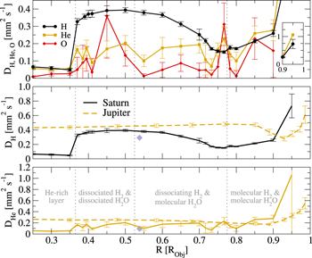
**Figure 8.** Self-diffusion coefficients D from DFT–MD for Saturn (solid lines) and Jupiter (French et al. 2012) (orange-dashed lines). Upper panel: D of hydrogen (black), helium (orange), and oxygen (red). The two lower panels show D_H and D_He, respectively. Blue diamonds denote interpolated data from DFT–MD results for a similar mixture with a higher content of heavy elements (Soubiran et al. 2017).
Download figure:
Standard image High-resolution image

The diffusion coefficient of hydrogen decreases with density in Saturn's outermost layer. It reaches a minimum at the onset of dissociation around R ≈ 0.75 R_S and then increases again as more and more molecules dissociate and become more mobile. The higher helium concentration in the He-rich layer decreases the mobility of the hydrogen atoms, which becomes visible at 0.45 R_S and cumulates in a significant decrease of D_H to a nearly constant value of 0.06 mm² s⁻¹ in the He-rich layer. The slope of D_H in Saturn is consistent with its slope in Jupiter, where the dissociation of hydrogen takes place at R ≈ 0.92 R_J and the influence of the He-rich layer is absent. Jupiter's higher temperatures result in higher particle velocities and therefore higher D_H.

While the values for the diffusion coefficient of hydrogen follow the slope of D_H in Jupiter at lower absolute values, the behavior of Saturn's D_He is more complex: In the He-rich layer, D_He ≈ D_H ≈ 0.06 mm² s⁻¹. Due to the comparatively low number of two to 10 helium atoms, D_He outside the He-rich layer is subject to large fluctuations, which can be seen in the slope shown in Figure 8.

This holds true for D_O as well, as the simulation boxes only contain one to three oxygen atoms. Therefore, those values represent only rough estimates for the tracer diffusion coefficient of oxygen in the H–He mixture.

Soubiran et al. (2017) performed DFT–MD simulations of a mixture of hydrogen, helium, and silicon dioxide. They calculated diffusion coefficients for hydrogen and helium at 5000 K, which corresponds to a pressure of ≈222 GPa and a radius coordinate of ≈0.54 in the MF20 model. We interpolated their diffusion coefficients for hydrogen and helium on the 5000 K isotherm to match the corresponding pressure of the MF20 model. Their lower hydrogen diffusivity originates from a greater amount of helium and heavy elements in their simulations. Their result for helium agrees with ours.

Wilson (2015) calculated diffusion coefficients for hydrogen, helium, carbon, silicon, and iron with DFT–MD. However, their lowest temperature under consideration was 10,000 K. Therefore, we do not compare their results to our data which range from around 2000 K to around 9000 K.

From the self-diffusion coefficients D_H and D_He, we can estimate the interdiffusion coefficient D_H,He via Darken's relation (Krishna & van Baten 2005; Liu et al. 2013). Together with the thermal diffusivity and viscosity, D_H,He can influence the convection behavior of the fluid, which might have a semiconvective or diffusive portion in certain parts of the planet (Stevenson & Salpeter 1977a; Rosenblum et al. 2011; Leconte & Chabrier 2012; Nettelmann et al. 2015; French & Nettelmann 2019).

4.3.2. Viscosity

We evaluate the shear viscosity η via a Green–Kubo formula employing autocorrelation functions of off-diagonal elements of the pressure tensor p_ij in the framework of linear response theory (Kubo 1957; Allen & Tildesley 1989; Alfè & Gillan 1998; French & Nettelmann 2019). We extract the pressure tensors from our DFT–MD simulations in thermodynamic equilibrium.

$\begin{eqnarray}&&\begin{array}{l}\eta =\displaystyle \frac{V}{3{k}_{{\rm{B}}}T}{\int }_{0}^{\infty }\ {d}t\ \displaystyle \sum _{\mathrm{ij}=\{{xy},{yz},{zx}\}}\ \langle ({p}_{\mathrm{ij}}(0)\\ -\,\langle {p}_{\mathrm{ij}}\rangle )\left({p}_{\mathrm{ij}}(t)-\langle {p}_{\mathrm{ij}}\rangle \right)\rangle .\end{array}\end{eqnarray} \tag{ 8 }$

Aside from p_ij, the dynamic shear viscosity η depends on the volume V of the simulation box, the Boltzmann constant k_B, the temperature T, and a sum over the directions xy, yz, and zx. Our conservative estimate of uncertainty for our results for the viscosities is 15%, except for the highest radius coordinate, where it is 50%. Figure 9 displays our results for the dynamic shear viscosity.

**Figure 9.** Dynamic shear viscosity η from DFT–MD for Saturn in black and Jupiter (French et al. 2012) in orange, compared to viscosity data for pure hydrogen from fitting to experimental data in blue (Stiel & Thodos 1963), and interpolated data from DFT–MD results for a similar mixture with a higher content of heavy elements (Soubiran et al. 2017) as light blue diamond.
Download figure:
Standard image High-resolution image

The DFT–MD results for the dynamic shear viscosity η in Jupiter increase with decreasing radius. Our results for Saturn follow the same slope and are systematically lower. In Saturn's He-rich layer, however, the density increase leads to values greater than those in Jupiter.

In a DFT–MD study of hydrogen, helium, and silicon dioxide under planetary interior conditions, Soubiran et al. (2017) also calculated the viscosity of their mixture at 5000 K. As mentioned in the discussion of Figure 8, we interpolated their data to a pressure of ≈222 GPa, which corresponds to a radius coordinate of ≈0.54 in the MF20 model. Their predicted viscosity is roughly 25% higher than our result at this radius coordinate, which is consistent with the greater amount of heavy elements in their simulations.

We additionally compare values extrapolated from low-density experimental data on pure hydrogen (Stiel & Thodos 1963). The extrapolated data feature significantly lower pressures than this study. We therefore compare the data at their highest pressure ≈130 kPa and the temperatures of the MF20 model between 0.522 and 0.98 R_S. Our result at 0.95 R_S agrees well with the extrapolated data. At lower radius coordinates the mixture becomes more correlated, resulting in increased viscosities, which is why our results differ from their low-density values.

Figure 10 shows our results for the kinematic shear viscosity ν = η/ρ. DFT–MD results for the kinematic shear viscosity in Jupiter are approximately constant and increase only slightly with radius. Our results for Saturn's He-rich layer exhibit a significantly higher ν than the predictions for Jupiter at the same relative radius coordinates. Our predictions for the dynamic shear viscosity in the layer of the dissociated fluid in Saturn coincide with Jovian values in the region directly above the He-rich layer. Their increase with radius is more pronounced than the predictions for Jupiter. Aside from our results for the He-rich layer, ν is almost constant within the uncertainties. Within the region that is most relevant for the operation of a dynamo, the approximation of a constant ν, which is a common assumption in dynamo modeling (Wicht & Tilgner 2010), is justified for Saturn according to our calculations.

Together with the higher density, the higher viscosity in the He-rich layer slows convection and might contribute to a stabilization of the layer within the planet.

4.3.3. Thermal Conductivity

We calculate the thermal conductivity as the sum of ionic and electronic contributions:

$\begin{eqnarray}&&\lambda ={\lambda }_{{\rm{i}}}+{\lambda }_{{\rm{e}}},\end{eqnarray} \tag{ 9 }$

$\begin{eqnarray}&&{\lambda }_{{\rm{i}}}=\displaystyle \frac{1}{3{{Vk}}_{{\rm{B}}}{T}^{2}}{\int }_{0}^{\infty }{d}t\ \langle {{\boldsymbol{J}}}_{q}^{{\prime} }(t)\cdot {{\boldsymbol{J}}}_{q}^{{\prime} }(0)\rangle ,\end{eqnarray} \tag{ 10 }$

$\begin{eqnarray}&&{\lambda }_{{\rm{e}}}=\mathop{\mathrm{lim}}\limits_{\omega \to 0}\displaystyle \frac{1}{T}\left({L}_{22}(\omega )-\displaystyle \frac{{L}_{12}^{2}(\omega )}{{L}_{11}(\omega )}\right).\end{eqnarray} \tag{ 11 }$

Here, the generalized heat currents ${{\boldsymbol{J}}}_{q}^{{\prime} }(t)$ and the Green–Kubo formula (Equation (10)) are evaluated as described by French (2019). Our estimate for the uncertainties in λ_i is 15%.

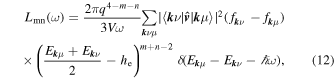
For the electronic contribution, we calculate the frequency-dependent Onsager coefficients L_mn(ω) from (Holst et al. 2011):

$\begin{eqnarray}&&\begin{array}{l}{L}_{\mathrm{mn}}(\omega )=\displaystyle \frac{2\pi {q}^{4-m-n}}{3V\omega }\displaystyle \sum _{{\boldsymbol{k}}\nu \mu }| \langle {\boldsymbol{k}}\nu | \hat{{\boldsymbol{v}}}| {\boldsymbol{k}}\mu \rangle {| }^{2}({f}_{{\boldsymbol{k}}\nu }-{f}_{{\boldsymbol{k}}\mu })\\ \times \,{\left(\displaystyle \frac{{E}_{{\boldsymbol{k}}\mu }+{E}_{{\boldsymbol{k}}\nu }}{2}-{h}_{{\rm{e}}}\right)}^{m+n-2}\ \delta \left({E}_{{\boldsymbol{k}}\mu }-{E}_{{\boldsymbol{k}}\nu }-{\hslash }\omega \right),\end{array}\end{eqnarray} \tag{ 12 }$

which contain the frequency ω, the charge q = −e, the electron mass m_e, a sum over the Bloch states ∣ k μ〉 with the occupation f_{k

μ} and the eigenenergies E_{k

μ}, the enthalpy per electron h_e, and the reduced Planck's constant ℏ.

The matrix elements $\langle {\boldsymbol{k}}\nu | \hat{{\boldsymbol{v}}}| {\boldsymbol{k}}\mu \rangle$ result from dipole matrix elements $\langle {\boldsymbol{k}}\nu | \hat{{\bf{r}}}| {\boldsymbol{k}}\mu \rangle$ ⁶ that take into account the nonlocal contributions from the Hartree–Fock exchange and from PAW potentials as implemented in the optical routines of VASP (Gajdoš et al. 2006; French & Redmer 2017).

We extract 30 ionic configurations from each of the DFT–MD simulations and then perform static DFT calculations with a Monkhorst–Pack (Monkhorst & Pack 1976) k-point sampling of 2 × 2 × 2. We use the HSE (Heyd et al. 2003, 2006) exchange-correlation functional with a Hartree–Fock screening parameter of 0.2 Å⁻¹ for a more accurate description of the band gap, and by extension, all electronic transport properties. Our estimated uncertainties for λ_e vary from 5%–50%, depending on the shape of the function we evaluate according to Equation (11).

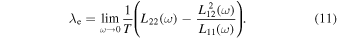
The relation between the thermal diffusivity κ and the thermal conductivity is

$\begin{eqnarray}&&\kappa =\displaystyle \frac{\lambda }{\rho {c}_{P}}.\end{eqnarray} \tag{ 13 }$

Figure 11 shows our results for the thermal conductivity λ and the thermal diffusivity κ.

In the molecular fluid of the outer layer, ionic contributions to the thermal conductivity dominate in our calculations. Upon the dissociation of molecular hydrogen, heat conduction from the electronic system becomes more pronounced and finally dominates in the dissociated fluid until the onset of the He-rich layer. Here, hydrogen molecules form in an atomic helium environment, which leads to only a few conducting electrons, and thus, a dominating λ_i. The thermal conductivity in Jupiter is significantly larger than in Saturn for R ≤ 0.90 R_Obj due to higher temperatures and pressures in Jupiter's interior.

The slopes for the thermal diffusivities κ from DFT–MD simulations are similar for Jupiter and Saturn. In the He-rich layer, however, κ is significantly smaller in Saturn than the thermal diffusivity in Jupiter due to the direct proportionality with the He layer's lower thermal conductivity λ, higher density, and lower heat capacity c_P at constant pressure (see Figure 4).

The He-rich layer exhibits a higher density, higher viscosity (see Section 4.3.2), and lower thermal conductivity than the layers above it. The corresponding reduction in heat flow from the hot core to the H–He envelope might have a significant impact on the cooling of the planet. To the best of our knowledge, this has never been accounted for in evolution studies for Saturn.

4.3.4. Static Electrical Conductivity

The static electrical (DC) conductivity σ follows from the static limit of the Onsager coefficient L₁₁(ω):

$\begin{eqnarray}&&\sigma =\mathop{\mathrm{lim}}\limits_{\omega \to 0}{L}_{11}(\omega ).\end{eqnarray} \tag{ 14 }$

We estimate the uncertainties, depending on the low-frequency behavior of L₁₁(ω), to be 5% in the metallic region between 0.733 and 0.37 R_S, 20% at 0.75 R_S, and 50% at all other radius coordinates. Figure 12 displays our results for σ.

**Figure 12.** DFT–MD results for the DC conductivity σ for Saturn (black) and Jupiter (French et al. 2012) (orange). Data shown in blue and light blue represent the results of earlier studies, obtained from calculations in the chemical picture, by Liu et al. (2008, 2014).
Download figure:
Standard image High-resolution image

Our results for σ have a slope similar to that of the results for Jupiter. The DC conductivity increases from the outer layer with increasing density. Due to a finer grid regarding radius coordinates, our results resolve a noticeable change in slope in the region of hydrogen dissociation. Our results predict an increase of σ in Saturn almost up to the values calculated for Jupiter (French et al. 2012). The electronically insulating helium in Saturn's He-rich layer results in a significant drop in σ by several orders of magnitude. The DC conductivity in the He-rich layer itself increases with density.

Results for the electronic contribution to the thermal conductivity (see Section 4.3.3) and the DC conductivity demonstrate that the He-rich environment deep in the planet impairs electronic transport, i.e., both electronic heat and charge conduction. Therefore, even if the He-rich layer was vigorously convective, it would barely contribute to the generation of Saturn's planetary magnetic field.

Liu et al. (2008, 2014) calculated interior models for Jupiter and Saturn based on the EOS of Saumon et al. (Saumon et al. 1995) and then inferred DC conductivities from a semiconductor model for hydrogen. Their earlier model (Liu et al. 2008) predicts DC conductivities in the molecular region that are systematically lower than our DFT–MD results but reproduces the slope of our results. Their later model (Liu et al. 2014) extends to smaller radius coordinates and features two distinct changes in slope; one around 0.85 R_S, which results from the onset of hydrogen metallization, and another around 0.6 R_S marking the full hydrogen metallization. Our ab initio simulations predict a comparable slope in the molecular region, and steeper slopes in the region of gradual hydrogen metallization as well as the fully dissociated regime. The main difference between our results and the Liu model is the location of the onset of hydrogen metallization at ≈0.775 R_S (Liu model: ≈0.85 R_S) and the location of full metallization at ≈0.7 R_S (Liu model: ≈0.615R_S).

The magnetic diffusivity β follows from σ according to

$\begin{eqnarray}&&\beta =\displaystyle \frac{1}{\sigma {\mu }_{0}},\end{eqnarray} \tag{ 15 }$

where μ₀ is the vacuum permittivity. Table 3 lists our results.

Table 3. Transport Properties in Saturn

R	D_H	D_He	η	ν	λ	κ	σ	β
[R_S]	[mm² s⁻¹]	[mm² s⁻¹]	[mPas]	[mm² s⁻¹]	[W (km)⁻¹]	[m² s⁻¹]	[MS m⁻¹]	[m² s⁻¹]
0.95	0.732	1.062	0.034	0.392	2.85	1.91 × 10⁻⁶	5.76 × 10⁻⁶	1.38 × 10¹¹
0.90	0.259	0.277	0.062	0.324	3.40	1.01 × 10⁻⁶	3.65 × 10⁻²	2.18 × 10⁷
0.85	0.214	0.259	0.126	0.438	3.01	6.39 × 10⁻⁷	3.00 × 10⁰	2.65 × 10⁵
0.80	0.171	0.100	0.173	0.448	3.11	4.87 × 10⁻⁷	9.93 × 10¹	8.01 × 10³
0.783	0.177	0.138	0.175	0.420	3.40	3.61 × 10⁻⁷	1.13 × 10³	7.02 × 10²
0.767	0.151	0.228	0.213	0.473	4.08	3.43 × 10⁻⁷	3.65 × 10³	2.18 × 10²
0.75	0.156	0.166	0.230	0.469	5.35	4.54 × 10⁻⁷	1.11 × 10⁴	7.19 × 10¹
0.733	0.170	0.069	0.244	0.460	9.77	6.89 × 10⁻⁷	4.34 × 10⁴	1.83 × 10¹
0.717	0.216	0.106	0.265	0.466	13.1	9.28 × 10⁻⁷	8.23 × 10⁴	9.67 × 10⁰
0.70	0.252	0.194	0.240	0.389	25.2	2.07 × 10⁻⁶	2.02 × 10⁵	3.94 × 10⁰
0.65	0.313	0.185	0.290	0.399	51.3	3.98 × 10⁻⁶	4.12 × 10⁵	1.93 × 10⁰
0.60	0.366	0.175	0.330	0.405	77.0	5.74 × 10⁻⁶	5.95 × 10⁵	1.34 × 10⁰
0.55	0.379	0.100	0.350	0.370	110	7.84 × 10⁻⁶	8.41 × 10⁵	9.46 × 10⁻¹
0.50	0.394	0.203	0.370	0.347	137	7.61 × 10⁻⁶	1.05 × 10⁶	7.58 × 10⁻¹
0.45	0.391	0.169	0.420	0.352	177	8.98 × 10⁻⁶	1.25 × 10⁶	6.37 × 10⁻¹
0.41	0.373	0.090	0.420	0.321	225	1.12 × 10⁻⁵	1.45 × 10⁶	5.49 × 10⁻¹
0.395	0.371	0.176	0.480	0.354	230	1.14 × 10⁻⁵	1.53 × 10⁶	5.20 × 10⁻¹
0.385	0.356	0.113	0.420	0.300	245	1.22 × 10⁻⁵	1.60 × 10⁶	4.97 × 10⁻¹
0.37	0.327	0.166	0.450	0.309	249	1.01 × 10⁻⁵	1.60 × 10⁶	4.97 × 10⁻¹
0.35	0.048	0.056	1.900	0.590	14.1	7.06 × 10⁻⁷	1.33 × 10²	5.99 × 10³
0.30	0.058	0.049	2.300	0.592	23.8	1.25 × 10⁻⁶	2.00 × 10³	3.98 × 10²
0.25	0.066	0.057	3.000	0.645	25.3	9.41 × 10⁻⁷	2.50 × 10³	3.18 × 10²

Download table as: ASCII Typeset image

Notice that our DFT–MD results for σ(R) (as well as other material properties reported in this work) along the P–T path for both planets are consistent with the corresponding EOS data. Other conductivity models in this parameter space are only valid for limiting cases. For instance, a multicomponent plasma model for the calculation of the composition and conductivity in the atmosphere of gas giants, in particular of hot Jupiters, has been developed recently (Kumar et al. 2021). The widely used Lee–More conductivity model (Lee & More 1984) is based on the relaxation time approximation and can only be applied to the fully ionized plasma in the deeper interior. Interpolation formulae for the electrical conductivity of strongly coupled, fully ionized plasmas based on correlation function approaches were derived for the same region (Ichimaru & Tanaka 1985; Röpke & Redmer 1989).

The Lorenz number L is a relation between electrical and thermal conductivities (Lorenz 1872):

$\begin{eqnarray}&&L=\displaystyle \frac{{e}^{2}}{{k}_{{\rm{B}}}^{2}}\displaystyle \frac{\lambda }{T\sigma }.\end{eqnarray} \tag{ 16 }$

In a completely degenerate electron gas, where only electrons are responsible for electrical and thermal conduction, like in metals and dense plasmas, L = π²/3 according to the Wiedemann–Franz law (Franz & Wiedemann 1853). When ions (or atoms and molecules) substantially contribute to the thermal conductivity, in weakly ionized gases or fluids, L can be orders of magnitude larger. Figure 13 displays our results for L.

**Figure 13.** Lorenz number L for Saturn (black) and Jupiter (French et al. 2012) (orange) from DFT–MD compared to the Wiedemann–Franz law (gray-dashed line). The inset shows the results for the outer layer.
Download figure:
Standard image High-resolution image

Our results for L in Saturn's He-rich layer are at least an order of magnitude larger than π²/3 due to the contributions of nonionized helium in the He-rich layer. In regions with smaller helium content, our values for L are closer to those in Jupiter. They reproduce the Wiedemann–Franz law within the uncertainties between the He-rich layer and the onset of hydrogen dissociation. However, L has large positive values in the lower He-rich and outer molecular layer, which is typical for the behavior of a semiconductor or a bad metal (Holst et al. 2011).

In light of the drastically lower electrical conductivity we find between R = 0.25 and 0.35 R_S as a result of helium sedimentation, it is clear that the processes in the region of Saturn's dynamo generation depend intimately on the H–He phase diagram. We encourage future magnetohydrodynamic studies to consider the effects of a deep insulating layer in which properties of helium dominate the properties of the H–He mixture due to the higher helium concentration. In particular, the apparent contradiction of Saturn's magnetic field with Cowling's theorem (axisymmetric with the rotation axis) has to be resolved by magnetohydrodynamic modeling, which can now be based on our ab initio database for material properties. Table 3 compiles our results for transport properties of matter in Saturn's interior.

5. Conclusions

We calculated thermodynamic and transport properties along the P–T path of a recent evolutionary Saturn model of MF20 in a range between 0.25 and 0.95 R_S. The MF20 model is based on ab initio data for the EOS (Becker et al. 2014) and the demixing diagram of hydrogen and helium (Schöttler & Redmer 2018). Both the EOS and the demixing diagram employed MD simulations based on a self-consistent quantum description of the electronic structure within DFT–MD.

Our findings significantly improve and enhance our knowledge about material properties (thermodynamic and transport) in Saturn. They provide robust results through the consistent use of DFT–MD throughout the generation of data for the MF20 model as well as for our calculation of material properties.

Compared to earlier results for Jupiter (French et al. 2012), the lower temperatures in the MF20 model lead to more pronounced implications of the insulator-to-metal phase transition on material and transport properties in the hydrogen-dominated outer layers of Saturn. We predict a significant impact of the metallization of hydrogen and the MF20 model's He-rich layer, especially on the thermal and electrical conductivity, as well as considerable consequences regarding the cooling behavior of Saturn.

Our results can serve as input for future models of Saturn's interior dynamics, especially hydrodynamic simulations for its magnetic field. Furthermore, they will help infer constraints for the interior structure and composition from future Saturn seismology data.

Acknowledgments

We thank M. Schörner, J. Wicht, and W. Dietrich for helpful discussions. This work was supported by the North German Supercomputing Alliance (HLRN) and the ITMZ of the University of Rostock as well as by the Deutsche Forschungsgemeinschaft (DFG) via the Research Unit FOR 2440.

Material Properties of Saturn's Interior from Ab Initio Simulations

Article metrics

Author e-mails

Author affiliations

ORCID iDs

Dates

Abstract

1. Introduction

2. Saturn Model

3. Ab Initio Simulations

4. Results