


Abstract
The solar magnetic field dominates solar activities in the solar atmosphere, such as solar flares and coronal mass ejections (CMEs). The Helioseismic and Magnetic Imager (HMI) on board the Solar Dynamics Observatory (SDO) has been in operation from 2010, providing a full-disk photospheric magnetogram. However, with a single view of observation, SDO/HMI cannot provide a global view of the Sun at the same time, so the farside of the Sun is blind to us. The Solar Terrestrial Relations Observatory (STEREO) provides two different views of the Sun with complementary viewing angles relative to SDO/HMI. However, it did not carry a magnetograph, but an extreme-ultraviolet (EUV) imager. Fortunately, deep learning has been proved to generate a solar farside magnetogram from STEREO farside EUV observation. Although a single generated magnetogram is morphologically very similar to ground truth, the sequence of the generated magnetogram has noticeable magnetic field fluctuation, which cannot be ignored when it is displayed as a time series, especially at an active region. This fluctuation is represented by sudden magnetic polarity reversal and drifting of magnetic field distribution. To mitigate this problem, a novel dynamic deep-learning model by integrating a convolutional gated recurrent units (convGRU) model into a pix2pix baseline is proposed in this paper. It can generate a sequence of a magnetogram with smooth transition among consecutive magnetograms by exploring spatio-temporal information of an input EUV image sequence. From both quantitative and qualitative comparisons, the proposed model can generate a magnetogram sequence more close to real observation.
Export citation and abstract BibTeX RIS

Original content from this work may be used under the terms of the Creative Commons Attribution 4.0 licence. Any further distribution of this work must maintain attribution to the author(s) and the title of the work, journal citation and DOI.
1. Introduction
A magnetic field manipulates all of the solar activities occurring in the solar atmosphere. Solar eruptions, such as flares and coronal mass ejections (CMEs), happening in the high solar atmosphere, are still highly associated with the photospheric magnetic field in the low solar atmosphere. Exploring the relation between the photospheric magnetic field and extreme-ultraviolet (EUV) observation of the corona is of great importance for us to understand the mechanism of solar eruptions, and further forecast them, preventing disastrous space weather from damaging high-tech systems.
The Solar Dynamics Observatory (SDO; Pesnell et al. 2012) was launched in 2010 February. One of its goals was for solar activity prediction. The Atmospheric Imaging Assembly (AIA) on the SDO can provide UV and EUV observations, which allows us to identify different kinds of solar chromosphere and corona structures. The Helioseismic and Magnetic Imager (HMI) can measure the photospheric magnetic field, providing a photospheric vector magnetogram. There exists a mapping between these two observations from the aspect of a physical mechanism (Galvez et al. 2019). It has been widely accepted that the whole solar atmosphere and solar activities are dominated by the solar magnetic field. Thus, UV/EUV emission of the corona can also provide clues of the magnetic field of the solar atmosphere.
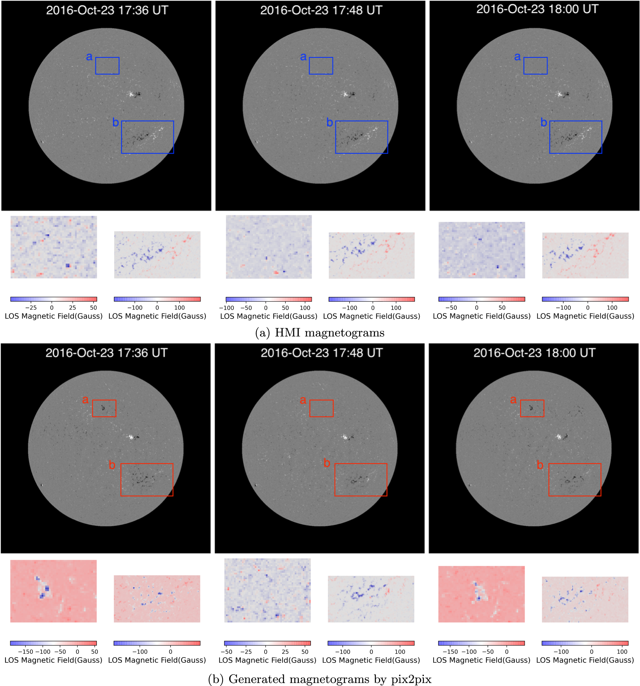
Kim et al. (2019) defined this mapping as an image-to-image translation, and applied the pix2pix model (Isola et al. 2017) to generate farside magnetograms from EUV observations to monitor the temporal evolution of an active region (AR) from the farside to the front side of the Sun. By the Kim et al. (2019) method, although each single generated magnetogram is morphologically very similar to ground truth, the composed sequence suffers from noticeable fluctuation of the magnetic field along the time, represented by shaking of the magnetic field, like a jitter in a video, while displaying the sequence. We name this phenomenon "magnetogram fluctuation" in this work. As demonstrated in Figure 1, three sequential HMI full-disk magnetograms and the corresponding ones generated by Kim et al. (2019) are listed in the first and third rows, respectively. To better tell the difference between them, two small patches highlighted by blue and red rectangles in the first and third rows are illustrated by color maps in the second and fourth rows of Figure 1. It can be observed that generated magnetograms have significantly larger differences than real observations. For example, by examining real observations from the first and second rows, patch (a) is in a quiet region of the solar disk. However, the generated one has significant variation of the magnetic field, exhibiting a very active magnetic field highlighted by red rectangles in the first and third columns. By checking patch (b) in the AR, real observation demonstrates a stable magnetic field in three consecutive magnetograms, while a generated one suffers from obvious polarity reversal and magnetic field variation.

Figure 1. The first and third rows show three sequential Helioseismic and Magnetic Imager (HMI) magnetograms and the ones generated by Kim et al. (2019), respectively. The second and fourth rows illustrate color maps of the two small patches labeled in the first and third rows, respectively.
Download figure:
Standard image High-resolution imageThe reason of magnetogram fluctuation may be twofold. First, the AIA and HMI record different physical parameters. The HMI (Scherrer et al. 2012) measures the polarization in a spectral line for studying all components of the photospheric magnetic field while the AIA (Lemen et al. 2012) provides narrow-band imaging of EUV and UV bandpasses to study the solar corona and transition region. The images of them are in different domains. Thus, there is a gap between the source domain and target domain as converting one to the other. Second, AIA observation records the source region of solar activity in the high solar atmosphere, such as solar flares and CMEs, while the HMI records the magnetic field of photosphere. Although there exists a mapping between AIA and HMI observations theoretically, they have totally different characteristics, expressing an asynchronous evolutionary rhythm and a different scale of variation. Once a solar flare/CME happens, the source region of the solar flare/CME would have sudden and intense heating in brightness and mass ejection in a short time, while the magnetic field of the corresponding photospheric regions still evolves at a small scale. To tackle these two problems, a dynamic model is proposed by additionally utilizing temporal evolution of input sequence to reduce fluctuation of output sequence. From our analysis, there exists a stable structure of long-term evolution in an EUV image sequence. However, the existing static model, namely Kim et al. (2019), lacks the mechanism for exploring evolution of input sequence.
Many problems in image processing have been enjoying considerable success in recent years because of the boom of deep learning (LeCun et al. 2015). The generative adversarial network (GAN; Goodfellow et al. 2014) is one of the most popular deep-learning models. It defines an adversarial framework consisting of a discriminator and a generator. By competing between the discriminator and the generator iteratively, GAN finally provides a powerful generator for image generation tasks. Compared to other networks, GAN could greatly ease the formulation and solving procedure of an optimization problem by adversarial learning. Out of these successful models, the pix2pix model proposed a generic framework of image-to-image translation based on the conditional GAN. This model can generate an image from sketch, reconstruct photos from edge maps, realize various image style transitions, and so on. However, the convolutional GAN fails to capture stable geometric or structural patterns of an image sequence since it is specialized to process image-like grid data instead of time series data (Goodfellow et al. 2016). This shortcoming leads to the failure of Kim's algorithm (Kim et al. 2019) for capturing stable chromosphere and corona structures from EUV observations. Besides, a solar event is described by a time series across a certain time interval. For studying solar events and the evolution of an AR, continuous observation and sequential images are needed. The SDO can provide continuous solar observation with high cadence. From the above analysis, we propose a convolutional gated recurrent units GAN by augmenting a general GAN with a convolutional gated recurrent units (convGRU; Cho et al. 2014), granting a GAN the ability of processing time series; convGRU is a lightweight recurrent neural network (RNN), superior to LSTM in some tasks (Chung et al. 2014).
Our main contribution is twofold in this paper. First, we explored an interesting phenomenon that a static model, like that in Kim et al. (2019), cannot generate a magnetogram sequence with the same evolution rate as the ground truth, resulting in magnetogram fluctuation. Second, a convGRU–GAN is proposed to generate a magnetogram sequence with stable evolution of the magnetic field, by integrating a convGRU into a general GAN. This remaining content is organized as follows. Section 2 introduces database and data preparation. Section 3 presents the details of a proposed model. The experimental setting and results are given in Section 4 and Section 5 draws the conclusion.
2. Data
We download SDO/AIA 304 Å and SDO/HMI line-of-sight magnetograms by using Sunpy (Community et al. 2015). First, We process level 1.5 images by calibrating, rotating, and centering. Since AIA and HMI instruments have different pixel resolution, we align HMI and AIA images such that they have the same spatial resolution. Then, we downsample them both to 512 × 512 (pixel resolution of 4.8'') by using the BICUBIC method (Keys 1981). Second, we normalize AIA 304 Å images by exposure time, and clip the HMI magnetogram within −200 G to 200 G. Considering elliptical orbital variation, we fix disk size Rs to 976'' (Galvez et al. 2019). After that, we double check the collected samples to exclude the samples with low quality or errors.
We concatenate three AIA 304 Å consecutive images together to compose a three-channel image. This three-channel image and one HMI image at the same time form an input–output pair for a training model, where the HMI image acts as the ground truth for a supervised learning purpose. Through above processing, 40,719 samples are collected to constitute a database with about 12 minutes cadence. For model training, we split the database into a training set, validation set, and testing set. The training set consists of samples from 2016 January 1, 00:00 UT to 2016 August 12, 13:48 UT. The validation set consists of samples from 2016 August 12, 14:24 UT to 2016 October 23, 16:24 UT. Then, the remaining samples form the testing set, to make sure there is no overlap between the training set and testing set. Thus, we have 24,435 samples for training, 8143 samples for validation, and 8141 samples for testing. The ratio of the number of samples among them is about 3:1:1.
3. Method
Kim et al. (2019) applied the pix2pix model to the AIA 304 Å image to generate a magnetogram with a photorealistic magnetic field. In general, a large scale structure of the solar magnetic field evolves slowly (Hoeksema 1984). However, the generated magnetogram sequence is plagued by magnetogram fluctuation as it is displayed as a time series, especially at an AR. To mitigate this problem, a dynamic model is constructed by combining a convGRU and a GAN in this work. It can manipulate sequence input and realize adversarial learning simultaneously. The principle behind the proposed model is to augment temporal context constraint (sequence input) into image generation to mitigate temporal fluctuation/jitter of the magnetogram sequence.
3.1. Pixpix Baseline
The pix2pix model has been widely recognized as a baseline of image translation. It is a conditional GAN, consisting of a generator and a discriminator. In a GAN framework, an adversarial loss optimizes a generator and a discriminator alternatively. The generator generates images that are so real that the discriminator cannot identify the real from the fake. Meanwhile, the discriminator improves itself, learning from cheating the generator over and over. Finally, a powerful generator can learn to translate the image of a source domain into the one of the target domain. In Kim et al. (2019), the generator is optimized to translate SDO/AIA images into HMI-like magnetograms, while the discriminator is adversarially optimized to distinguish between real and generated magnetograms.
The objective of a conditional GAN can be expressed by

where G is a generator and D is a discriminator; G tries to minimize the objective function against an adversarial D. In (1), x is the input (AIA 304 Å), y is the ground truth (HMI magnetogram), and G(x) is the output of the generator G. In addition, L1 regularization rather than L2 regularization was employed as L1 could encourage less blurring of a generated magnetogram (Isola et al. 2017), which is defined by

Therefore, the final objective function is given by

The pix2pix model adopts a U-Net framework as the generator and a patch-wised fully convolutional network as the discriminator. However, such a static model cannot capture stable geometric or structural patterns by local convolution kernels. The HMI records the solar magnetic field of photosphere where large scale structure evolves slowly (Hoeksema 1984). Compared to the HMI, the AIA records solar activities at a high solar atmosphere, where sudden brightening or mass ejection usually happens. In this sense, there is a certain gap between source domain (AIA) and target domain (HMI) concerning the image translation task. To bridge this gap, we attempt to propose a dynamic/time series model to explore sequential attribute of input AIA image sequence to guide magnetogram generation. By this way, we can alleviate the asynchronization between AIA and HMI sequences so that the generated magnetogram sequence has a relatively stable evolution.
3.2. Convolutional GRU
The RNN is a time series model for processing sequential input. However, it is prone to an exploding or vanishing gradient during the model training process (Bengio et al. 1994). In response, variants of RNNs were raised, such as LSTM (Hochreiter & Schmidhuber 1997) and GRU. They demonstrate superiority of modeling long-term temporal dependency in various tasks, such as neural machine translation and speech recognition. In this work, GRU is employed due to the efficiency comparable to LSTM and the lower memory requirement (Chung et al. 2014). It has a gating structure for controlling the flow of information inside the units. It is formulated as

where xt , ht , rt , and zt denote input, hidden activation, reset gate value, and update gate value, respectively; W* and R* are the weights imposed on input and recurrent hidden units. The symbols σ and ⊙ represent a sigmoid function and an element-wise multiplication, respectively.
Ballas et al. (2015) has explored GRU to the convolutional version (namely convGRU) for video representation. The convGRU extended the GRU–RNN model and replaced the fully connected RNN linear product operation with a convolution. It can encode the locality and temporal smoothness priors of an image sequence, so it is well suited for capturing fine motion information. For this very reason, it is selected to explore sudden and large scale variation of an AIA image sequence.
3.3. Network Architecture
As mentioned above, a static model, like pix2pix, cannot capture stable geometric or structural patterns of an image sequence by local convolution kernels. Compared to the HMI image sequence, the AIA image sequence has a fast local brightening or fast coronal mass ejection, resulting in asynchronization of them. To realize the translation between them, the proposed model is expected to be capable of capturing long-term evolution of stable structures of the AIA image sequence. Thus, a dynamic deep-learning model by integrating convGRU into pix2pix is proposed in this work, namely convGRU–pix2pix. It consists of a generator and a discriminator, and accepts image sequence input. The schematic diagram of convGRU–pix2pix is illustrated in Figure 2. The proposed convGRU–pix2pix in general is an encoder–decoder system. The encoder extracts compressed features/representations of input AIA image, and the decoder unpacks the compressed features to generate a HMI-like magnetogram, while the convGRU cell in between takes a sequence of image features as input to extract a long-term stable structure from the input. The network architecture of the generator of convGRU–pix2pix is shown in Figure 3, which is basically a U-Net in shape, while augmented with a convGRU unit at the bottom of the U-Net.

Figure 2. Diagram of magnetogram generation from Atmospheric Imaging Assembly (AIA) image sequence.
Download figure:
Standard image High-resolution image
Figure 3. Network architecture of convGRU–pix2pix.
Download figure:
Standard image High-resolution image4. Experiments
The proposed model is implemented on Pytorch (Paszke et al. 2019). It relies on a number of parameters that are obtained through our extensive experiments. The slope of LeakyReLu is 0.2, and the dropout probability is 0.5. The epoch is set to 200, which indicates the number of training iterations over the training data set. The learning rate is a hyperparameter that controls how much the model changes for each time of weights updating, which is initially set to 0.0002, and decays to half after 100 epochs. The batch size denotes the number of samples participating in training for each iteration, which is set to four for the balance between computational complexity and model performance. The model takes AIA image sequence as input, where sequence length is empirically set to three considering model complexity and performance.
Two sets of experiments, full-disk and AR magnetograms, are conducted to evaluate our model. In Section 4.1, our model can generate full-disk magnetograms with visually pleasant perceptual quality and higher objective quality. In Section 4.2, it can be observed that our model can obtain more stable evolution of ARs than the others.
4.1. Full-disk Evaluation
The proposed convGRU–pix2pix is compared with the other two benchmarks: pix2pix baseline and multichannel pix2pix. Pix2pix baseline is the same as the original one (Isola et al. 2017), while multichannel pix2pix has the same setting as pix2pix baseline except for the input. The proposed model takes the same input as multichannel pix2pix, namely the AIA 304 Å image sequence. In Figure 4, we compare the ground truth (HMI magnetograms) and generated ones among different models. When displaying the sequence of generated magnetograms, it can be found that the proposed model has less fluctuation of magnetic polarities and stable structure evolution than the others. For example, patch (a) is in the quiet region, while the strong magnetic field emerges for pix2pix in Figure 4(c). By examining patch (b) among compared methods, our model produces the magnetograms well matched with the ground truth (Figure 1(a)), with a clear magnetic field boundary and magnetic field polarity as shown in Figure 4(a). Although multichannel pix2pix also takes image sequence input, it lacks the mechanism of learning sequential features from sequence input, resulting in fluctuation of the magnetic field. It turns out that the convGRU module really makes sense for capturing the sequential features of input sequence.

Figure 4. Comparisons of generated magnetograms among the proposed convGRU–pix2pix, multichannel pix2pix, and pix2pix baseline. To tell "magnetogram fluctuation" more clearly, the color maps of the two small patches labeled by "a" and "b" are illustrated next to each full-disk magnetogram.
Download figure:
Standard image High-resolution imageFor objective evaluation, the generated magnetograms are compared with the ground truth with respect to six objective metrics: the structural similarity index measure (SSIM), peak signal-to-noise ratio (PSNR), total unsigned magnetic flux correlation coefficient (cc), positive flux cc, and negative cc. Among them, SSIM and PSNR are the most common metrics in image processing, which are defined by

where x and y represent an observed magnetogram and generated one, respectively, μx
and μy
are the means of x and y, respectively,  and
and  are the variances of x an y, respectively, σxy
is the covariance of x and y, c1 and c2 are two constant parameters to stabilize the division with a weak denominator. Following the setting of original authors, c1 and c2 are 2.55 and 7.65, respectively. SSIM is more likely to reflect the structural similarity of two images. PSNR is defined by mean squared error (MSE) and maximum pixel value (MaxValue) of an image in (5). It qualifies the pixel-to-pixel difference between the generated image and the ground truth. In our case, the maximum pixel value of the magnetogram is 200 (MaxValue = 200). The statistics of six objective metrics are listed in Table 1, where "STD" represents standard deviation, which is computed by
are the variances of x an y, respectively, σxy
is the covariance of x and y, c1 and c2 are two constant parameters to stabilize the division with a weak denominator. Following the setting of original authors, c1 and c2 are 2.55 and 7.65, respectively. SSIM is more likely to reflect the structural similarity of two images. PSNR is defined by mean squared error (MSE) and maximum pixel value (MaxValue) of an image in (5). It qualifies the pixel-to-pixel difference between the generated image and the ground truth. In our case, the maximum pixel value of the magnetogram is 200 (MaxValue = 200). The statistics of six objective metrics are listed in Table 1, where "STD" represents standard deviation, which is computed by  over 8141 test samples.
Table 1. Objective Comparisons among Pix2pix, Multichannel Pix2pix, and Our Model over 8141 Test Samples
| SSIM/STD | PSNR/STD | Total Unsigned | Positive Flux cc | Negative Flux cc | |
|---|---|---|---|---|---|
| Magnetic Flux cc | |||||
| Pix2pix baseline | 0.84 +/− 0.0062 | 33.84 +/− 0.58 | 0.80 | 0.79 | 0.81 |
| Multichannel pix2pix | 0.87 +/− 0.0037 | 32.85 +/− 0.85 | 0.66 | 0.70 | 0.73 |
| ConvGRU–pix2pix (ours) | 0.89 +/− 0.0037 | 34.64 +/− 0.53 | 0.88 | 0.87 | 0.89 |
Download table as: ASCIITypeset image
From Table 1, our proposed model achieves the best SSIM and PSNR (the least MSE), which is consistent with subjective evaluation. In addition, the total unsigned flux cc, positive flux cc, and negative flux cc are up to 0.88, 0.87, and 0.89 for our model. They are all much larger than those of the others, indicating that our model is highly consistent with the ground truth.
4.2. Active Region Evaluation
We further examine AR magnetogram generation. Getting coordinates of ARs from Spaceweather HMI Active Region Patch (SHARP), we cut corresponding ARs from HMI full-disk magnetograms to provide testing samples. These testing samples are from 2016 October 23, 17:00 UT to 2016 December 31, 23:48 UT. During this period, there are two M-class flares, one is M1.0 and the other is M1.5.
The SHARP ARs numbered 6838, 6846, 6863, 6868, and 6870 are selected for both subjective and objective analysis. Each of them consists of about 300–700 frames. In Table 2, average SSIM and PSNR, as well as their STDs are listed for each AR. It is notable that in Table 2, not only do the metrics show improved values using the proposed algorithm but also that the standard deviations are also less, indicating similar performance over the frames of an AR sequence.
Table 2. Average SSIM and PSNR and Their STDs are Compared among Pix2pix Baseline, Multichannel Pix2pix, and Our Model
| Active Region | SHARP 6838 | SHARP 6846 | SHARP 6863 | SHARP 6868 | SHARP 6870 | |
|---|---|---|---|---|---|---|
| SSIM | Pix2pix baseline | 0.49 +/− 0.10 | 0.39 +/− 0.09 | 0.49 +/− 0.52 | 0.45 +/− 0.10 | 0.36 +/− 0.09 |
| Multichannel pix2pix | 0.46 +/− 0.10 | 0.37 +/− 0.11 | 0.36 +/− 0.04 | 0.42 +/− 0.11 | 0.33 +/− 0.09 | |
| ConvGRU–pix2pix (ours) | 0.55 +/− 0.03 | 0.46 +/− 0.04 | 0.54 +/− 0.02 | 0.52 +/− 0.04 | 0.41 +/− 0.04 | |
| PSNR | Pix2pix baseline | 21.43 +/− 1.75 | 19.52 +/− 1.40 | 21.68 +/− 0.49 | 20.22 +/− 1.50 | 17.62 +/− 2.42 |
| Multichannel pix2pix | 20.89 +/− 1.85 | 19.20 +/− 1.54 | 18.76 +/− 0.75 | 19.73 +/− 1.58 | 16.79 +/− 2.50 | |
| ConvGRU–pix2pix (ours) | 22.43 +/− 1.06 | 20.56 +/− 0.59 | 21.99 +/− 0.55 | 21.11 +/− 0.53 | 19.08 +/− 0.92 | |
Download table as: ASCIITypeset image
In Figure 5, the ground truth and three compared methods are illustrated for the selected ARs mentioned above, where the first column lists the ground truth (HMI magnetogram), and the other columns are our model, multichannel pix2pix, and pix2pix baseline, respectively. For easily examining AR sequence evolution, the difference between two consecutive magnetograms, namely "magnetogram difference," is computed and illustrated by a color map in the row next to each AR sequence. From Figure 5, it can be observed that our model is more morphologically close to the ground truth by comparing their color maps. To measure such a similarity, the pixel-to-pixel cc between the color maps of the ground truth and each compared algorithm is computed. In addition, we can also notice that positive and negative polarities (bright spots and dark spots) are well matched between our model and the ground truth.

Figure 5. Subjective comparison among the ground truth, our model, multichannel pix2pix, and pix2pix baseline. (Magnetogram difference describes the difference between two consecutive frames of an AR sequence. It is illustrated by a color map. To better characterize the morphological similarity between the color maps of real observed data and generated ones from different models, pixel-to-pixel correlation coefficient (cc) between two compared color maps is computed and labeled accordingly.)
Download figure:
Standard image High-resolution image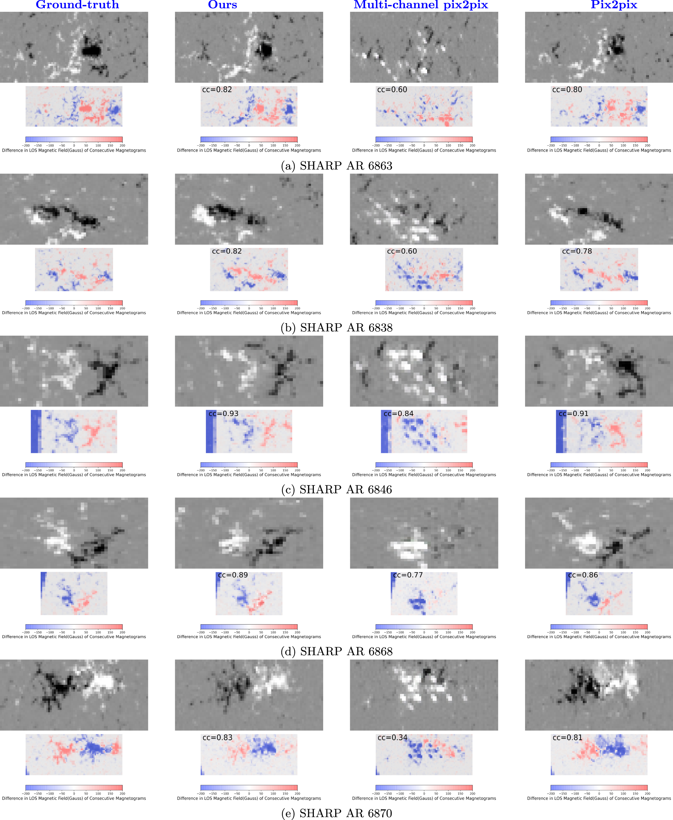
5. Conclusion
In this paper, a dynamic deep-learning model, namely convGRU–pix2pix, is proposed to address the problem of magnetogram fluctuation in Kim et al. (2019). Extensive verification indicates that the proposed model can achieve a more stable evolution of the magnetic field from sequence input of SDO/AIA 304 Å, with less magnetogram fluctuation and more consistent polarity distribution to the ground truth. In addition, we also verify the efficiency of our model for generating an AR in this paper, which is more challenging.
Thanks to the editor and reviewer for their suggestions for improving our manuscript. We thank the Solar Activity Prediction Group members for their helpful academic discussions, comments, and suggestions about this work. We thank Xingyao Chen, Peijin Zhang for their helpful discussion and encouragement. This work was supported by the National Key R&D Program of China (No. 2021YFA1600500, 2021YFA1600504), the Peng Cheng Laboratory Cloud Brain (No. PCL2021A13), the CAAI-Huawei MindSpore Open Fund, the National Natural Science Foundation of China (NSFC) (No. 11790300, 11790305, 61902371).