


Abstract
This paper reports computational results on hydrogen Lyman β, γ, and Balmer β spectral lines in the presence of parallel magnetic and electric fields. A two-dimensional B-spline approach is adopted in the current calculations. This approach was originally developed to treat high-lying states but was found to be also effective for low-lying states. Wavelengths and oscillator strengths are presented for a total of 31 transitions in magnetic and electric fields with field strengths ranging, respectively, from 23.5 to 2350 MG and from 0 to 108 V m−1. These spectral data are compared to available results from other theoretical methods, and good agreement is clearly visible. Our calculations show that in the scope of field strengths we are concerned with, Lyman β and γ spectral lines lie in the ultraviolet region, while the Balmer β lines lie in the ultraviolet and visible-light regions. Furthermore, Zeeman spectral lines related to atomic states in the n = 4 manifold may be blue- or redshifted by a strong electric field, dependent on the transitions as well as on magnetic field strengths. Atomic spectral data of the 31 transitions listed are applicable for modeling discrete spectra of magnetic white dwarfs when a strong electric field exists in the hydrogen-dominated atmospheres of these celestial objects.
Export citation and abstract BibTeX RIS

Original content from this work may be used under the terms of the Creative Commons Attribution 4.0 licence. Any further distribution of this work must maintain attribution to the author(s) and the title of the work, journal citation and DOI.
1. Introduction
Understanding the behavior of atoms in external magnetic and electric fields is of fundamental physics interest. Such an atomic system has attracted considerable attention since the early 1970s. Demkov et al. (1970) first formulated the energy level splitting of hydrogen in magnetic and electric fields of arbitrary mutual orientation within the framework of perturbation theory, and the symmetry of the four-dimensional Fock rotation group was adopted in their formulation. Soon afterward, a quasiclassical calculation was also reported for atomic states of H-like systems in crossed electric and magnetic fields (Burkova et al. 1976). Relevant experimental progress lagged behind theoretical work due to the difficulty of experimental techniques. Up until the 1980s, high-resolution laser spectroscopy setups were being constructed to study the problem of atoms in the presence of magnetic and electric fields (Cacciani et al. 1986). Photoexcitation spectra of lithium in parallel external fields below the field-free ionization threshold were recorded, and the structures of energy spectra belonging to high-n manifolds of lithium were systematically investigated as a function of the intensity of one of the two fields, with the other one being kept constant in Cacciani et al. (1986, 1988).
The development of the experimental technique mentioned above further stimulated interest in atoms in external fields. This atomic system may serve as a potential tool to investigate chaotic phenomena because of its unique characteristics. Main & Wunner (1992) was dedicated to this type of study by selecting photoionization processes of hydrogen in crossed magnetic and electric fields. A quantum calculation of photoionization cross sections was performed using the complex-coordinate-rotation method, and strong Ericson fluctuations, a characteristic feature of chaotic scattering, were found in the calculated photoionization spectra. This theoretical prediction was first observed by Stania & Walther (2005) in a photoionization experiment of rubidium atoms in strong crossed fields. Hydrogen in two kinds of external fields with an arbitrary mutual orientation is a more general system than that in crossed magnetic and electric fields, and hence photoionization for such a system was selected by Main et al. (1998) to further deeply understand chaotic phenomena. The dependence of photoionization spectra on the mutual orientation of two kinds of external fields was studied. Their calculations of eigenenergies show strong level repulsions around the Stark saddle point, namely the so-called avoided crossings. The large avoided crossings are believed to be a quantum manifestation of the classical intramanifold chaos.
To explain the experimental photoabsorption spectra of multielectronic atoms, as reported in Cacciani et al. (1986, 1988), the R-matrix method combined with the quantum-defect theory was formulated by Santos et al. (1999) to describe the behavior of multielectronic atoms in parallel electric and magnetic fields. This theoretical approach can be regarded as an extension of the previous adiabatic-basis-expansion method, which was originally developed by Mota-Furtado & O'Mahony (1991) to calculate the photoionization of atoms and molecules in a pure magnetic field with terrestrial laboratory strengths, and later applied to calculations of continuum spectra of atoms in white dwarf magnetic field strengths (Mota-Furtado & O'Mahony 2007; Zhao et al. 2021; Zhao 2021a). Using this approach, Santos et al. (1999) presented photoionization spectra for Li and Rb in parallel external fields and gave a detailed analysis of nonhydrogenic characters of the spectra for Li and Rb. Their computational spectra were compared to high-precision experimental ones, and good agreement was found.
The discovery of strong magnetic fields in extremely dense celestial objects, the so-called magnetic white-dwarf and neutron stars (Garstang 1977), further strengthened interest in the problem of atoms in magnetic and electric fields. The magnetic fields of these celestial objects can be determined from Zeeman spectral lines calculated and astronomically observed in their atmospheres, while the magnetic fields are crucial to understanding their evolution from normal stars to white-dwarf and neutron stars (Garstang 1977). A variety of theoretical studies have been hitherto performed to calculate the atomic structures and spectra in a wide range of magnetic fields (see Ruder et al. 1994 and references therein). Substantial headway was made on the simulation of spectra for hydrogen in an arbitrary magnetic field (see, e.g., Forster et al. 1984; Rösner et al. 1984; Baye et al. 2008a, 2008b; Schimeczek & Wunner 2014a, 2014b; Zhao & Liu 2019; Liu & Zhao 2020), and thus the identification of discrete spectral lines for any transition of magnetized hydrogen has become practicable in white-dwarf and neutron stars with hydrogen-dominated atmospheres.
As more and more white dwarfs were classified as magnetic (Ferrario et al. 2015, 2020), some magnetized multielectronic atoms were identified in the atmospheres of white dwarfs. For example, discrete spectral lines of Na i, Mg i, Al i, Ca ii, and Fe i in the cool magnetic white dwarf NLTT 7547 (Kawka et al. 2019) and lines of Na i, Mg i, Ca i, and Ca ii were observed in the magnetic DZ white dwarf LHS 2534 (Reid et al. 2000). In the current stage, however, electron correlation is effectively treated only in several few-electron atoms in magnetic fields of white-dwarf and/or neutron stars, such as He and Li (see, e.g., Becken et al. 1999; Zhao 2018, and references therein), and calculations of magnetized multielectronic atoms depend mainly on the Hartree–Fock theory, which is not able to produce spectral data with the sufficient accuracy required in astronomy and astrophysics. The progress on the observation of spectral lines in magnetic white dwarfs poses a big challenge to theorists, who are inevitably confronted with the difficult problem of electron correlation in a strong magnetic field.
Notwithstanding significant success in the simulation of atomic spectral lines in a pure magnetic field with arbitrary strength, distinct discrepancies were noticed between the computed and observed spectra in some magnetic white dwarfs. For example, absorption spectra for two stationary transitions, 2s0 → 3p0 and 2s0 → 4f0, observed in the hydrogen-dominated atmosphere of Grw+70.8247 were found to shift about 5–6 Å with respect to the computed spectra (Friedrich et al. 1994). The reasons that give rise to the distinct discrepancies have been analyzed by Friedrich et al. (1994) and Fassbinder & Schweizer (1996a). Their analyses show that an additional electric field, which may be caused by free electrons and ions in the stellar atmosphere or motional Stark effects, should be responsible for the discrepancies. The electric field strength was believed to be of the order of 106–109 V m−1.
Fassbinder & Schweizer (1996a) theoretically studied the problem of hydrogen in strong magnetic and electric fields with arbitrary mutual orientation using a discrete variable representation (DVR) method. The DVR method was first developed by Melezhik (1993) to calculate atomic structures of hydrogen in external magnetic and electric fields, and then soon extended by Fassbinder & Schweizer (1996a) to simulate discrete spectral lines of this system observed in white-dwarf stars. It was found that in the range of white-dwarf field strengths, the influence of the perpendicular component of an arbitrarily oriented electric field on wavelengths and oscillator strengths is negligible. This important conclusion makes it much easier to describe hydrogen in magnetic and electric fields because the problem of hydrogen in two kinds of fields with arbitrary mutual orientation is able to be simplified to that in parallel external fields. Soon afterward, Fassbinder & Schweizer (1996b) reduced their three-dimensional discretization method to a two-dimensional one and calculated stationary spectral lines in parallel magnetic and electric fields. Wavelengths and oscillator strengths of Lyman α, and Balmer α and Balmer β lines were presented as a function of white-dwarf-strength magnetic and electric fields.
Guan & Zhang (2004) formulated a two-dimensional discretization pseudospectral method to understand the influence of an additional electric field on Zeeman spectral lines of hydrogen atoms in a magnetic field. These two fields are parallel with each other, and their field strengths are taken in the regions with magnetic fields B ≤ 470 MG and electric fields F ≤ 108 V m−1. Oscillator strength spectra were reported for Balmer α transitions of hydrogen atoms in parallel fields as a function of magnetic and electric field strengths. Based on the pseudospectral discretization technique, Guan (2006) developed two independent methods to study the more general problem of hydrogen in crossed magnetic and electric fields with arbitrary mutual orientation, and spectra of the Balmer α series in crossed fields were computed using the two methods. Special attention was paid to the effect of electric fields with arbitrary orientation on hydrogen Zeeman spectral lines in Guan (2006), and the perpendicular component of an electric field was found to give rise to a weaker coupling between atomic states belonging to different subspaces of magnetic quantum numbers. This conclusion is similar to that obtained by Fassbinder & Schweizer (1996a).
To the best of our knowledge, theoretical results available in the literature are far from satisfying the requirements for astronomical application. A comprehensive compilation of atomic spectral data containing all transitions in magnetic and electric fields is obviously essential. Recently, the two-dimensional B-spline approach, which was previously developed to describe lithium atoms in a pure magnetic field (Zhao 2020, 2021b), was extended to calculate hydrogen in parallel magnetic and electric fields (Zhao & Liu 2021). Wavelengths and oscillator strengths were presented for spectral lines of 14 Balmer α transitions as a function of white-dwarf-strength magnetic and electric fields. In this paper, we will apply the extended approach to calculations of spectral lines of Lyman α, β, γ, and Balmer β transitions of hydrogen atoms in parallel magnetic and electric fields. However, we will not list here the atomic data of Lyman α lines because the influence of an electric field with strength F ≤ 108 eV on their wavelengths and oscillator strengths is trivial.
The remainder of this paper is organized as follows. Section 2 outlines the two-dimensional B-spline approach utilized in this work, including the theoretical description of hydrogen atoms in parallel magnetic and electric fields, the numerical solution of the two-dimensional Schrödinger equation, and the calculations of the spectral lines. Section 3 is devoted to a detailed presentation of the calculated spectral lines for a total of 31 transitions of hydrogen atoms in parallel magnetic and electric fields. Our spectral data are also compared with available results in the literature in this section. The main results of this work are summarized, and concluding remarks concerning the influence of an additional electric field on spectral lines of hydrogen atoms in pure magnetic fields are given in Section 4. Atomic units are used throughout unless otherwise noted.
2. Approach
We recapitulate in this section the two-dimensional B-spline approach utilized in the current work. This approach was previously developed to calculate the Zeeman spectra of lithium atoms in a pure white-dwarf-strength magnetic field (Zhao 2020, 2021b), following the formulation of Schimeczek & Wunner (2014a). Very recently, it has been extended to describe hydrogen atoms in parallel magnetic and electric fields (Zhao & Liu 2021).
2.1. Hamiltonian and Symmetries of Hydrogen in Parallel Fields
Let us take into account an atomic system of hydrogen in the presence of external magnetic B and electric fields F, with the directions of both fields selected to point toward the direction of the z-axis. Our theoretical description of this system begins by assuming that the nuclear mass is infinite and its relativistic effects, such as spin–orbit coupling, are negligible. In this assumption, the Hamiltonian of this system can be written in cylindrical coordinates as

where γ = B/B0 and  denote the magnetic and electric field strengths with
  T and
T and  V m−1, and
  and
and  are the z components of the orbital and spin angular momenta, respectively. In Equation (1), the third term linear in γ is the paramagnetic potential, the fourth term quadratic in γ is the diamagnetic potential, and the term
  represents the interaction of the hydrogen atom with the electric field. Note that energies in Equation (1) are measured in units of Hartrees. For the hydrogen atom in a pure magnetic field, i.e.,
  in Equation (1) is removed,
  ,
,  , and the parity in the z direction πz
are constants of motion for the Hamiltonian.
, and the parity in the z direction πz
are constants of motion for the Hamiltonian.
It is easily seen that if an additional parallel electric field is added to a hydrogen atom exposed to a magnetic field, the parity symmetry of this atomic system is no longer maintained, but  and
and  are still conserved quantities. As a consequence of the conservation of the z component of the orbital angular momentum, the three-dimensional Schrödinger equation for the Hamiltonian (1) can be reduced to a two-dimensional problem, while the two-dimensional Schrödinger equation is no longer separable due to the existence of magnetic fields, and thus it becomes inevitable that two-dimensional differential equations will need to be solved.
2.2. Solution of the Two-dimensional Schrödinger Equation
We select a finite basis set from B-spline functions to solve the two-dimensional Schrödinger equations. Concerning the B-spline functions, many types of computer programs have been written for the purpose of calculations. This kind of function was initially introduced in the 1950s, and a surge of applications of B-splines in many fields appeared in the 1990s with the advent of powerful computers (Bachau et al. 2001). Their properties have been detailed in de Boor (2001), and a FORTRAN code to produce B-spline functions with any order is given in that book. In particular, applications of B-splines in atomic and molecular physics have been reviewed by Bachau et al. (2001). Details on computing magnetized atoms using B-splines are also available in Zhao & Stancil (2007).
Our procedure for determining the eigenvalues and eigenfunctions of the Hamiltonian (1) starts from expanding the wave function Ψ(ρ, z, ϕ) in the ρ − z plane of the cylindrical coordinate system in terms of B-spline functions Bi,k of order k,

where m represents the magnetic quantum number corresponding to  , and Bi,k
(z) and Bi,k
(ρ) are located in limited regions with
, and Bi,k
(z) and Bi,k
(ρ) are located in limited regions with  and
and  , respectively. Substituting Equation (2) into the Schrödinger equation for Hamiltonian (1), multiplying the resulting equation by
  for each
  and each
  , and then integrating each of the obtained equations over ρ and z, we obtain a generalized eigenvalue equation set. Using a compact matrix notation, the generalized eigenvalue equation set is written as

where H and  are the Hamiltonian and overlap matrices. The expressions of their matrix elements have been given in Zhao (2020) and hence are not listed here again. We would like to emphasize that the overlap matrix
  is reduced to an identity matrix if the nonorthogonal B-spline basis is replaced by an orthogonal basis set.
The solution of any eigenvalue or generalized eigenvalue problem inevitably involves applying suitable boundary conditions. The details to enforce the physical boundary conditions of the problem given in Equation (3) have been illustrated in Zhao & Liu (2021) and hence are not repeated here. We adopt the Gaussian quadratures (Press et al. 1992) to compute each matrix element of H and  . Once numerical calculations of all matrix elements are finished, we utilize the Cholesky matrix factorization technique to transfer the generalized eigenvalue problem into an eigenvalue problem and then solve the resulting eigenvalue equations. Note that we will not directly factorize
  and instead factorize two small-size overlap submatrices belonging to the ρ and z coordinates,
  and
and  , in order to save computing time. It can be demonstrated that
  is the Kronecker product of
  and
and  , i.e.,
  , while it is much faster to compute the Cholesky matrix factorization of
  from the two submatrices
  and
and  than directly factorize
  .
.
2.3. Oscillator Strengths for Dipole Transitions in Parallel Fields
Using energy eigenvalues and eigenvectors obtained by solving the generalized eigenvalue problem, Equation (3), wavelengths and oscillator strengths of spectral lines for any transition of hydrogen in parallel magnetic and electric fields can be computed. Considering the fact that the m degeneracy in the field-free case is entirely removed when an atom is placed in an external magnetic field, an averaging procedure over m in the initial and final atomic states is no longer required, and therefore the oscillator strength for a dipole transition from an initial state Ψi to a final state Ψf is written in the form

where Ei and Ef denote the energy levels for the initial and final states, respectively, and D is the dipole operator, defined in the cylindrical coordinate system as

specifying the interaction of atoms with the radiation field.
3. Results and Discussion
A crucial step of atomic structure calculations with a finite basis set from B-spline functions is to choose a suitable knot sequence {ti
} in a limited region, according to the distribution of wave functions. For the system of hydrogen atoms in parallel magnetic and electric fields, a scheme to distribute the knot sequences on both the ρ- and z-axes with a linearly increasing spacing was found to be an efficient scheme (Zhao & Liu 2021), which was first introduced by Schimeczek & Wunner (2014a) to describe hydrogen in a pure magnetic field. This distribution scheme of the knot sequences on both the ρ- and z-axes is adopted in the current work, and ρ and z are supposed to be located in a limited range, [0, ![${\rho }_{\max }]$](https://content.cld.iop.org/journals/0067-0049/259/2/47/revision1/apjsac4ca2ieqn32.gif) and
and  , zmax], respectively.
For the system of atoms in a pure magnetic field, the integration in the z coordinate involved in calculations of all matrix elements of H and  can be restricted to z ≥ 0, as done in Schimeczek & Wunner (2014a, 2014b) and Zhao (2021b). It is reasonable to impose this restriction because the parity under the reflection of the wave function about the z = 0 plane is a conserved quantity in this case. However, if an additional electric field is added, the parity symmetry in the z direction is broken, and as a consequence, such a restriction is no longer valid. In such a case, one has to perform integration from
  to zmax. The feature that the parity symmetry no longer remains for the system of atoms in external magnetic and electric fields leads to greatly increasing the number of the B-spline basis and the size of the Hamiltonian matrix, and thus computing time is remarkably increased compared to the case of atoms in a pure magnetic field.
Our aim in the current work lies in the Lyman α, β, γ, and Balmer β spectral lines of hydrogen in parallel magnetic and electric fields, as these lines are relevant to the atomic states in the n = 1–4 manifolds. Note that the hydrogen Balmer α spectral lines in parallel fields have already been reported (Zhao & Liu 2021), and thus it is not required to recalculate their atomic states in the n = 2 and 3 manifolds related to these Balmer α lines. Only atomic states in the n = 1 and 4 manifolds are to be calculated. These states will be optimized based on the following steps. For each atomic state of a given magnetic field and a given electric field, we vary  , zmax, and the knot sequences on both the ρ- and z-axes to seek the optimized eigenvalue of the atomic state. Furthermore, we also check the convergence of the current problem by means of increasing the number Nρ
and order kρ
of B-spline functions on the ρ-axis, and the number Nz
and order kz
of B-spline functions on the z-axis.
, zmax, and the knot sequences on both the ρ- and z-axes to seek the optimized eigenvalue of the atomic state. Furthermore, we also check the convergence of the current problem by means of increasing the number Nρ
and order kρ
of B-spline functions on the ρ-axis, and the number Nz
and order kz
of B-spline functions on the z-axis.
The present optimal calculations of atomic structures begin from selecting reasonable initial values of the following parameters,  , zmax, Nρ
, and Nz
. Doing so can save a lot of computing time. Small and large initial values of these parameters should be taken, respectively, for low- and high-lying atomic states. For example, for the high-lying
, zmax, Nρ
, and Nz
. Doing so can save a lot of computing time. Small and large initial values of these parameters should be taken, respectively, for low- and high-lying atomic states. For example, for the high-lying  state at γ = 0.01 au and F = 108 V m−1, we took these initial values be
  , zmax = 100, Nρ
= 32, and Nz
= 62. By increasing the four parameters up to 120, 150, 72, 152, we found that a convergent energy eigenvalue of eight significant digits, −0.038259232 au, is obtained at
, zmax = 100, Nρ
= 32, and Nz
= 62. By increasing the four parameters up to 120, 150, 72, 152, we found that a convergent energy eigenvalue of eight significant digits, −0.038259232 au, is obtained at  , zmax = 100, Nρ
= 52, and Nz
= 102. It should be mentioned that convergence with only five significant digits is reached using the initial values of these parameters.
, zmax = 100, Nρ
= 52, and Nz
= 102. It should be mentioned that convergence with only five significant digits is reached using the initial values of these parameters.
We make use of the notation of Fassbinder & Schweizer (1996b),  , to specify atomic states in parallel magnetic and electric fields throughout this paper. This notation with the prime distinguishes that in a pure magnetic field, n
ℓm (see, e.g., Rösner et al. 1984). We optimized atomic states in the n = 1 and 4 manifolds,
, to specify atomic states in parallel magnetic and electric fields throughout this paper. This notation with the prime distinguishes that in a pure magnetic field, n
ℓm (see, e.g., Rösner et al. 1984). We optimized atomic states in the n = 1 and 4 manifolds,  ,
,  ,
,  , and
, and  , for given magnetic and electric field strengths. The field strengths range, respectively, from 23.5 to 2350 MG, and from 0 to 108 V m−1. Notice that we did not include
  because ionization of this state begins to be significant for not very low electric field strengths. It is well known that an atomic system placed in an electric field may ionize by tunneling through the potential barrier. If the energy level of this system approaches, and in particular is above, the classical saddle point
  , its ionization becomes so fast that it is imperative to include continuum channels in the wave function. In such a case, it is inappropriate to treat the atomic state as a bound state anymore. However, it is not the aim of this work to treat tunneling through the potential barrier, so our current calculations drop those spectral lines related to
  .
.
To understand the spectral line shifts caused by electric fields, it is obviously helpful to explore the influence of electric fields on the atomic states of hydrogen in a magnetic field. We illustrate the variation of atomic states of magnetized hydrogen in n = 4 manifolds with electric fields. Contour plots of probability density distributions for two states  and
and  are shown in Figures 1 and 2. We selected three magnetic field strength values of γ = 0.01, 0.1, and 1.0 au and drew plots of F = 0, 106, 107, and 108 V m−1 for each γ value. From these two figures, one can see a definite symmetry of atomic states with respect to the inversion of z for each γ value of these two states at F = 0 V m−1, but such a definite symmetry is clearly broken by a strong electric field. For a given γ, the asymmetry of atomic states becomes more and more remarkable as electric fields increase.

Figure 1. Probability densities of the atomic state  in parallel magnetic and electric fields. The field strengths are taken to be γ = 0.01, 0.1, and 1.0 au and F = 0, 106, 107, and 108 V m−1.
Download figure:
Standard image High-resolution image
Figure 2. Same as Figure 1, but for state  .
.
Download figure:
Standard image High-resolution imageThe probability density distributions for the two n = 4 manifold states at γ = 1.0 au and F = 108 V/cm are discovered to obviously deviate from symmetry with respect to the inversion of z. This case is different from that of the n = 3 manifold states. The influence of electric fields on the probability density distributions for  was noticed to be imperceptible at the same field strengths (Zhao & Liu 2021). This is attributed to their different energy levels. The atomic states
  and
and  of higher energy levels are more easily affected than the
  of lower energy levels. For a given strong electric field, the variation of electron cloud distributions with γ is also visible. One can see from the last column of Figure 1 that the electron clouds are distributed almost under the z = 0 plane at γ = 0.01 au but are primarily above the z plane at γ = 0.1 au, and again primarily under the z = 0 plane at γ = 1.0 au. Such a variation is the result of competition among the Coulombic force, the Lorentz force, and the electrostatic field force. A similar phenomenon was also found by Paradis et al. (2013). They show that the calculated normalized electron wave function probabilities of Rb atoms in parallel magnetic and electric fields are distributed not only under but also above the z = 0 plane under different conditions.
Using atomic structure data in the n = 1–4 manifolds obtained, spectral lines of two transitions,  and
and  , are first calculated. Our current calculations show that the influence of electric fields with strengths F ≤ 108 V m−1 on Zeeman spectral lines of Lyman α transitions is trivial. The very same conclusion was also drawn by Fassbinder & Schweizer (1996b). They discovered that only for very strong electric fields do the wavelengths of spectral lines of Lyman α transitions show an observable variation. For example, an electric field of strength F = 109 V m−1 was found to give rise to a redshift of about 0.4 Å for the transition
  . In view of the rather small influence of electric fields on Lyman α lines, it is superfluous to tabulate Lyman α lines in electric fields of strengths F ≤ 108 V m−1.
Let us then move on to Lyman β, γ, and Balmer β spectral lines in parallel fields. Wavelengths and oscillator strengths for a total of 31 transitions of these three spectral series are calculated and presented in Tables 1–31 as a function of magnetic and electric field strengths. The 31 transitions include 16 special transitions, which are dipole-forbidden in a pure magnetic field, such as  and
and  . Only when an electric field is added do these dipole-forbidden transitions in a pure magnetic field become allowed. Our oscillator strengths calculated for 16 special transitions are found to increase by several orders of magnitude when increasing electric fields from F = 106 to 108 V m−1. From the current results and those reported in Zhao & Liu (2021), it can be concluded that only in the case of relatively high electric fields are spectral lines for dipole-forbidden transitions in a pure magnetic field strong enough to be visible in celestial observations. It is worth mentioning that in the scope of field strengths illustrated in these tables, the Lyman β and γ spectral lines lie in the ultraviolet region, while the Balmer β lines in the ultraviolet and visible-light regions.
Table 1. Wavelengths λ in Angstroms and Oscillator Strengths f, Listed in the Upper and Lower Rows, for Transition  , as a Function of Magnetic Field Strengths γ in Atomic Units and Electric Field Strengths F in 107 V m−1
| Electric Field Strength F (107 V m−1) | ||||||||
|---|---|---|---|---|---|---|---|---|
| γ (au) | 0 | 0.1 | 1.0 | 2.0 | 4.0 | 6.0 | 8.0 | 10.0 |
| 0.01 | 1020.90 | 1020.90 | 1020.88 | 1020.83 | 1020.59 | 1020.16 | 1019.59 | 1018.93 |
| 0 | 6.607(−6) | 6.660(−4) | 2.716(−3) | 1.096(−2) | 2.157(−2) | 2.953(−2) | 3.423(−2) | |
| 0.02 | 1009.68 | 1009.68 | 1009.67 | 1009.66 | 1009.61 | 1009.52 | 1009.39 | 1009.22 |
| 0 | 5.745(−7) | 5.748(−5) | 2.304(−4) | 9.284(−4) | 2.112(−3) | 3.799(−3) | 5.996(−3) | |
| 0.03 | 994.31 | 994.31 | 994.31 | 994.30 | 994.28 | 994.24 | 994.19 | 994.12 |
| 0 | 1.800(−7) | 1.801(−5) | 7.207(−5) | 2.889(−4) | 6.522(−4) | 1.165(−3) | 1.830(−3) | |
| 0.04 | 977.08 | 977.08 | 977.08 | 977.08 | 977.07 | 977.06 | 977.04 | 977.01 |
| 0 | 1.123(−7) | 1.123(−5) | 4.497(−5) | 1.803(−4) | 4.073(−4) | 7.282(−4) | 1.146(−3) | |
| 0.05 | 959.89 | 959.89 | 959.90 | 959.90 | 959.91 | 959.92 | 959.95 | 959.98 |
| 0 | 1.359(−7) | 1.359(−5) | 5.446(−5) | 2.192(−4) | 4.982(−4) | 8.987(−4) | 1.432(−3) | |
| 0.06 | 944.54 | 944.54 | 944.55 | 944.56 | 944.62 | 944.73 | 944.89 | 945.10 |
| 0 | 2.817(−7) | 2.818(−5) | 1.129(−4) | 4.542(−4) | 1.032(−3) | 1.856(−3) | 2.939(−3) | |
| 0.07 | 932.04 | 932.04 | 932.06 | 932.09 | 932.25 | 932.51 | 932.88 | 933.35 |
| 0 | 5.790(−7) | 5.783(−5) | 2.305(−4) | 9.088(−4) | 1.995(−3) | 3.423(−3) | 5.102(−3) | |
| 0.08 | 921.75 | 921.75 | 921.77 | 921.83 | 922.07 | 922.46 | 922.98 | 923.63 |
| 0 | 8.728(−7) | 8.696(−5) | 3.441(−4) | 1.319(−3) | 2.775(−3) | 4.523(−3) | 6.381(−3) | |
| 0.09 | 912.63 | 912.63 | 912.65 | 912.73 | 913.02 | 913.48 | 914.09 | 914.82 |
| 0 | 1.065(−6) | 1.059(−4) | 4.165(−4) | 1.563(−3) | 3.192(−3) | 5.033(−3) | 6.878(−3) | |
| 0.10 | 904.11 | 904.11 | 904.13 | 904.22 | 904.54 | 905.04 | 905.70 | 906.48 |
| 0 | 1.182(−6) | 1.174(−4) | 4.597(−4) | 1.699(−3) | 3.398(−3) | 5.245(−3) | 7.030(−3) | |
| 0.20 | 830.14 | 830.14 | 830.23 | 830.45 | 831.17 | 832.06 | 833.02 | 834.03 |
| 0 | 7.232(−6) | 6.668(−4) | 2.169(−3) | 5.105(−3) | 6.989(−3) | 8.127(−3) | 8.832(−3) | |
| 0.30 | 770.51 | 770.51 | 770.46 | 770.31 | 769.83 | 769.18 | 768.48 | 767.75 |
| 0 | 3.621(−6) | 3.491(−4) | 1.262(−3) | 3.723(−3) | 6.038(−3) | 8.012(−3) | 9.824(−3) | |
| 0.40 | 724.87 | 724.87 | 724.86 | 724.81 | 724.62 | 724.34 | 724.02 | 723.72 |
| 0 | 1.237(−6) | 1.229(−4) | 4.816(−4) | 1.790(−3) | 3.642(−3) | 5.796(−3) | 8.103(−3) | |
| 0.50 | 688.54 | 688.54 | 688.54 | 688.51 | 688.42 | 688.29 | 688.16 | 688.07 |
| 0 | 9.240(−7) | 9.210(−5) | 3.648(−4) | 1.406(−3) | 2.990(−3) | 4.958(−3) | 7.115(−3) | |
| 0.60 | 658.32 | 658.32 | 658.32 | 658.31 | 658.26 | 658.20 | 658.15 | 658.15 |
| 0 | 7.989(−7) | 7.971(−5) | 3.167(−4) | 1.233(−3) | 2.661(−3) | 4.467(−3) | 6.463(−3) | |
| 0.70 | 632.52 | 632.52 | 632.52 | 632.52 | 632.49 | 632.47 | 632.46 | 632.50 |
| 0 | 7.255(−7) | 7.241(−5) | 2.880(−4) | 1.127(−3) | 2.445(−3) | 4.128(−3) | 5.996(−3) | |
| 0.80 | 610.11 | 610.11 | 610.11 | 610.11 | 610.10 | 610.09 | 610.11 | 610.17 |
| 0 | 6.745(−7) | 6.734(−5) | 2.680(−4) | 1.051(−3) | 2.288(−3) | 3.874(−3) | 5.643(−3) | |
| 0.90 | 590.38 | 590.38 | 590.38 | 590.37 | 590.37 | 590.38 | 590.41 | 590.48 |
| 0 | 6.359(−7) | 6.349(−5) | 2.528(−4) | 9.928(−4) | 2.165(−3) | 3.673(−3) | 5.363(−3) | |
| 1.00 | 572.81 | 572.81 | 572.81 | 572.81 | 572.81 | 572.83 | 572.87 | 572.94 |
| 0 | 6.051(−7) | 6.042(−5) | 2.406(−4) | 9.459(−4) | 2.065(−3) | 3.510(−3) | 5.134(−3) | |
Download table as: ASCIITypeset image
Table 2. Similar to Table 1, but for Transition 
| Electric Field Strength F (107 V m−1) | |||||||||
|---|---|---|---|---|---|---|---|---|---|
| γ (au) | 0 | 0 a | 0.1 | 1.0 | 2.0 | 4.0 | 6.0 | 8.0 | 10.0 |
| 0.01 | 1023.24 | 1023.2353 | 1023.23 | 1023.13 | 1022.91 | 1022.48 | 1022.19 | 1022.05 | 1021.98 |
| 8.117(−2) | 8.117 3943(−2) | 8.103(−2) | 7.086(−2) | 5.790(−2) | 3.973(−2) | 2.529(−2) | 1.548(−2) | 9.801(−3) | |
| 0.02 | 1018.13 | 1018.1266 | 1018.13 | 1018.09 | 1017.99 | 1017.64 | 1017.20 | 1016.74 | 1016.28 |
| 8.542(−2) | 8.541 7107(−2) | 8.540(−2) | 8.413(−2) | 8.078(−2) | 7.200(−2) | 6.402(−2) | 5.746(−2) | 5.181(−2) | |
| 0.03 | 1011.12 | 1011.1182 | 1011.12 | 1011.10 | 1011.04 | 1010.82 | 1010.49 | 1010.09 | 1009.65 |
| 8.912(−2) | 8.912 2895(−2) | 8.912(−2) | 8.871(−2) | 8.753(−2) | 8.352(−2) | 7.852(−2) | 7.355(−2) | 6.901(−2) | |
| 0.04 | 1003.17 | 1003.1686 | 1003.17 | 1003.15 | 1003.11 | 1002.95 | 1002.70 | 1002.37 | 1001.99 |
| 9.119(−2) | 9.119 3495(−2) | 9.119(−2) | 9.098(−2) | 9.037(−2) | 8.810(−2) | 8.489(−2) | 8.128(−2) | 7.761(−2) | |
| 0.05 | 994.84 | 994.841 26 | 994.84 | 994.83 | 994.80 | 994.66 | 994.45 | 994.18 | 993.85 |
| 9.166(−2) | 9.166 4697(−2) | 9.166(−2) | 9.153(−2) | 9.111(−2) | 8.956(−2) | 8.725(−2) | 8.447(−2) | 8.148(−2) | |
| 0.06 | 986.43 | 986.432 70 | 986.43 | 986.42 | 986.39 | 986.28 | 986.09 | 985.84 | 985.54 |
| 9.099(−2) | 9.099 0527(−2) | 9.099(−2) | 9.088(−2) | 9.057(−2) | 8.935(−2) | 8.749(−2) | 8.519(−2) | 8.264(−2) | |
| 0.07 | 978.09 | 978.088 49 | 978.09 | 978.08 | 978.05 | 977.95 | 977.77 | 977.54 | 977.26 |
| 8.965(−2) | 8.964 5832(−2) | 8.964(−2) | 8.955(−2) | 8.928(−2) | 8.823(−2) | 8.661(−2) | 8.458(−2) | 8.228(−2) | |
| 0.08 | 969.88 | 969.875 40 | 969.88 | 969.87 | 969.84 | 969.74 | 969.57 | 969.35 | 969.07 |
| 8.799(−2) | 8.798 5720(−2) | 8.798(−2) | 8.790(−2) | 8.765(−2) | 8.667(−2) | 8.516(−2) | 8.326(−2) | 8.109(−2) | |
| 0.09 | 961.82 | 961.821 60 | 961.82 | 961.81 | 961.79 | 961.68 | 961.51 | 961.29 | 961.01 |
| 8.624(−2) | 8.623 5152(−2) | 8.623(−2) | 8.615(−2) | 8.590(−2) | 8.494(−2) | 8.345(−2) | 8.157(−2) | 7.944(−2) | |
| 0.10 | 953.94 | 953.937 05 | 953.94 | 953.93 | 953.90 | 953.79 | 953.62 | 953.38 | 953.10 |
| 8.452(−2) | 8.452 1015(−2) | 8.452(−2) | 8.443(−2) | 8.417(−2) | 8.316(−2) | 8.161(−2) | 7.967(−2) | 7.750(−2) | |
| 0.20 | 883.94 | 883.942 42 | 883.94 | 883.96 | 884.03 | 884.26 | 884.61 | 885.03 | 885.50 |
| 7.354(−2) | 7.354 4325(−2) | 7.354(−2) | 7.315(−2) | 7.205(−2) | 6.843(−2) | 6.418(−2) | 6.023(−2) | 5.686(−2) | |
| 0.30 | 827.40 | 827.401 85 | 827.40 | 827.41 | 827.42 | 827.47 | 827.55 | 827.67 | 827.82 |
| 6.896(−2) | 6.895 8801(−2) | 6.896(−2) | 6.893(−2) | 6.886(−2) | 6.858(−2) | 6.812(−2) | 6.749(−2) | 6.672(−2) | |
| 0.40 | 781.02 | 781.020 18 | 781.02 | 781.02 | 781.03 | 781.06 | 781.11 | 781.18 | 781.26 |
| 6.645(−2) | 6.644 8463(−2) | 6.645(−2) | 6.644(−2) | 6.640(−2) | 6.625(−2) | 6.601(−2) | 6.568(−2) | 6.526(−2) | |
| 0.50 | 742.29 | 742.291 24 | 742.29 | 742.29 | 742.30 | 742.32 | 742.35 | 742.40 | 742.47 |
| 6.480(−2) | 6.480 1670(−2) | 6.480(−2) | 6.479(−2) | 6.477(−2) | 6.466(−2) | 6.449(−2) | 6.424(−2) | 6.394(−2) | |
| 0.60 | 709.40 | 709.401 16 | 709.40 | 709.40 | 709.41 | 709.42 | 709.45 | 709.49 | 709.54 |
| 6.361(−2) | 6.360 5391(−2) | 6.361(−2) | 6.360(−2) | 6.358(−2) | 6.349(−2) | 6.335(−2) | 6.315(−2) | 6.290(−2) | |
| 0.70 | 681.05 | 681.048 65 | 681.05 | 681.05 | 681.05 | 681.07 | 681.09 | 681.12 | 681.16 |
| 6.268(−2) | 6.268 0862(−2) | 6.268(−2) | 6.267(−2) | 6.266(−2) | 6.258(−2) | 6.246(−2) | 6.229(−2) | 6.207(−2) | |
| 0.80 | 656.29 | 656.289 65 | 656.29 | 656.29 | 656.29 | 656.31 | 656.32 | 656.35 | 656.39 |
| 6.194(−2) | 6.193 6331(−2) | 6.194(−2) | 6.193(−2) | 6.191(−2) | 6.185(−2) | 6.174(−2) | 6.158(−2) | 6.139(−2) | |
| 0.90 | 634.43 | 634.427 05 | 634.43 | 634.43 | 634.43 | 634.44 | 634.46 | 634.48 | 634.51 |
| 6.132(−2) | 6.131 8798(−2) | 6.132(−2) | 6.131(−2) | 6.130(−2) | 6.124(−2) | 6.114(−2) | 6.100(−2) | 6.082(−2) | |
| 1.00 | 614.94 | 614.936 20 | 614.94 | 614.94 | 614.94 | 614.95 | 614.96 | 614.98 | 615.01 |
| 6.079(−2) | 6.079 4991(−2) | 6.079(−2) | 6.079(−2) | 6.078(−2) | 6.072(−2) | 6.063(−2) | 6.050(−2) | 6.033(−2) | |
Note.
a This column represents electric-field-free calculations from the finite-basis-set method (Zhao & Liu 2019).Download table as: ASCIITypeset image
Table 3. Similar to Table 1, but for Transition 
| Electric Field Strength F (107 V m−1) | ||||||||
|---|---|---|---|---|---|---|---|---|
| γ (au) | 0 | 0.1 | 1.0 | 2.0 | 4.0 | 6.0 | 8.0 | 10.0 |
| 0.01 | 1024.06 | 1024.06 | 1024.19 | 1024.47 | 1025.17 | 1025.93 | 1026.72 | 1027.53 |
| 0 | 1.413(−4) | 9.648(−3) | 2.055(−2) | 3.046(−2) | 3.427(−2) | 3.606(−2) | 3.699(−2) | |
| 0.02 | 1020.95 | 1020.95 | 1020.99 | 1021.12 | 1021.54 | 1022.11 | 1022.76 | 1023.46 |
| 0 | 1.285(−5) | 1.233(−3) | 4.400(−3) | 1.247(−2) | 1.924(−2) | 2.408(−2) | 2.749(−2) | |
| 0.03 | 1016.29 | 1016.29 | 1016.31 | 1016.38 | 1016.65 | 1017.06 | 1017.56 | 1018.14 |
| 0 | 3.985(−6) | 3.935(−4) | 1.517(−3) | 5.305(−3) | 9.924(−3) | 1.436(−2) | 1.821(−2) | |
| 0.04 | 1010.49 | 1010.49 | 1010.50 | 1010.55 | 1010.75 | 1011.06 | 1011.46 | 1011.94 |
| 0 | 2.016(−6) | 2.004(−4) | 7.865(−4) | 2.929(−3) | 5.922(−3) | 9.244(−3) | 1.252(−2) | |
| 0.05 | 1003.85 | 1003.85 | 1003.86 | 1003.90 | 1004.06 | 1004.32 | 1004.65 | 1005.07 |
| 0 | 1.318(−6) | 1.313(−4) | 5.187(−4) | 1.978(−3) | 4.134(−3) | 6.692(−3) | 9.394(−3) | |
| 0.06 | 996.60 | 996.60 | 996.61 | 996.64 | 996.78 | 997.01 | 997.31 | 997.68 |
| 0 | 1.009(−6) | 1.005(−4) | 3.983(−4) | 1.535(−3) | 3.258(−3) | 5.370(−3) | 7.682(−3) | |
| 0.07 | 988.89 | 988.89 | 988.90 | 988.93 | 989.06 | 989.27 | 989.55 | 989.89 |
| 0 | 8.602(−7) | 8.579(−5) | 3.403(−4) | 1.318(−3) | 2.817(−3) | 4.684(−3) | 6.764(−3) | |
| 0.08 | 980.85 | 980.85 | 980.86 | 980.89 | 981.02 | 981.21 | 981.48 | 981.82 |
| 0 | 7.975(−7) | 7.955(−5) | 3.157(−4) | 1.225(−3) | 2.624(−3) | 4.377(−3) | 6.342(−3) | |
| 0.09 | 972.57 | 972.57 | 972.58 | 972.61 | 972.73 | 972.93 | 973.20 | 973.53 |
| 0 | 7.934(−7) | 7.913(−5) | 3.140(−4) | 1.217(−3) | 2.607(−3) | 4.343(−3) | 6.285(−3) | |
| 0.10 | 964.12 | 964.12 | 964.13 | 964.17 | 964.29 | 964.49 | 964.76 | 965.10 |
| 0 | 8.427(−7) | 8.403(−5) | 3.332(−4) | 1.288(−3) | 2.747(−3) | 4.554(−3) | 6.555(−3) | |
| 0.20 | 879.90 | 879.90 | 879.88 | 879.82 | 879.59 | 879.26 | 878.86 | 878.42 |
| 0 | 3.951(−6) | 3.892(−4) | 1.490(−3) | 5.102(−3) | 9.329(−3) | 1.326(−2) | 1.659(−2) | |
| 0.30 | 811.44 | 811.44 | 811.43 | 811.42 | 811.38 | 811.31 | 811.22 | 811.11 |
| 0 | 2.558(−7) | 2.557(−5) | 1.021(−4) | 4.054(−4) | 9.016(−4) | 1.577(−3) | 2.416(−3) | |
| 0.40 | 760.51 | 760.51 | 760.51 | 760.50 | 760.49 | 760.46 | 760.43 | 760.38 |
| 0 | 1.511(−7) | 1.511(−5) | 6.040(−5) | 2.411(−4) | 5.404(−4) | 9.558(−4) | 1.484(−3) | |
| 0.50 | 720.57 | 720.57 | 720.57 | 720.57 | 720.56 | 720.55 | 720.54 | 720.53 |
| 0 | 1.216(−7) | 1.216(−5) | 4.864(−5) | 1.943(−4) | 4.363(−4) | 7.735(−4) | 1.204(−3) | |
| 0.60 | 687.68 | 687.68 | 687.68 | 687.68 | 687.68 | 687.68 | 687.68 | 687.68 |
| 0 | 1.065(−7) | 1.065(−5) | 4.258(−5) | 1.702(−4) | 3.823(−4) | 6.783(−4) | 1.057(−3) | |
| 0.70 | 659.79 | 659.79 | 659.79 | 659.79 | 659.79 | 659.79 | 659.79 | 659.80 |
| 0 | 9.652(−8) | 9.652(−6) | 3.860(−5) | 1.543(−4) | 3.467(−4) | 6.153(−4) | 9.592(−4) | |
| 0.80 | 635.65 | 635.65 | 635.65 | 635.65 | 635.65 | 635.66 | 635.67 | 635.67 |
| 0 | 8.921(−8) | 8.921(−6) | 3.568(−5) | 1.426(−4) | 3.205(−4) | 5.688(−4) | 8.869(−4) | |
| 0.90 | 614.46 | 614.46 | 614.46 | 614.47 | 614.47 | 614.47 | 614.48 | 614.49 |
| 0 | 8.350(−8) | 8.349(−6) | 3.339(−5) | 1.335(−4) | 3.000(−4) | 5.325(−4) | 8.304(−4) | |
| 1.00 | 595.65 | 595.65 | 595.65 | 595.65 | 595.65 | 595.66 | 595.67 | 595.68 |
| 0 | 7.886(−8) | 7.885(−6) | 3.154(−5) | 1.261(−4) | 2.834(−4) | 5.030(−4) | 7.844(−4) | |
Download table as: ASCIITypeset image
Table 4. Similar to Table 2, but for Transition 
| Electric Field Strength F (107 V m−1) | |||||||||
|---|---|---|---|---|---|---|---|---|---|
| γ (au) | 0 | 0a | 0.1 | 1.0 | 2.0 | 4.0 | 6.0 | 8.0 | 10.0 |
| 0.01 | 965.21 | 965.208 44 | 965.21 | 965.20 | 965.16 | 964.89 | 964.27 | 963.44 | 962.63 |
| 1.949(−2) | 1.949 0833(−2) | 1.949(−2) | 1.963(−2) | 1.998(−2) | 2.001(−2) | 1.668(−2) | 1.214(−2) | 7.986(−3) | |
| 0.02 | 951.30 | 951.302 63 | 951.30 | 951.30 | 951.31 | 951.33 | 951.36 | 951.39 | 951.49 |
| 1.339(−2) | 1.339 1728(−2) | 1.339(−2) | 1.339(−2) | 1.336(−2) | 1.326(−2) | 1.295(−2) | 1.206(−2) | 9.158(−3) | |
| 0.03 | 936.82 | 936.816 06 | 936.82 | 936.84 | 936.91 | 937.22 | 937.85 | 938.98 | 940.71 |
| 2.397(−3) | 2.397 0112(−3) | 2.396(−3) | 2.339(−3) | 2.165(−3) | 1.489(−3) | 5.649(−4) | 1.348(−5) | 1.691(−4) | |
| 0.04 | 924.11 | 924.104 60 | 924.11 | 924.20 | 924.50 | 925.58 | 927.17 | 929.12 | 931.35 |
| 1.324(−3) | 1.324 3573(−3) | 1.325(−3) | 1.378(−3) | 1.529(−3) | 1.984(−3) | 2.390(−3) | 2.541(−3) | 2.306(−3) | |
| 0.05 | 913.14 | 913.144 31 | 913.15 | 913.39 | 914.00 | 915.70 | 917.68 | 919.85 | 922.19 |
| 9.220(−3) | 9.219 5380(−3) | 9.212(−3) | 8.614(−3) | 7.651(−3) | 6.392(−3) | 5.594(−3) | 4.821(−3) | 3.791(−3) | |
| 0.06 | 903.34 | 903.340 48 | 903.35 | 903.73 | 904.52 | 906.42 | 908.50 | 910.71 | ⋯ |
| 1.536(−2) | 1.536 0650(−2) | 1.532(−2) | 1.301(−2) | 1.066(−2) | 8.285(−3) | 6.806(−3) | 5.385(−3) | ⋯ | |
| 0.07 | 894.32 | 894.320 94 | 894.33 | 894.68 | 895.43 | 897.28 | 899.28 | 901.36 | ⋯ |
| 1.775(−2) | 1.774 8691(−2) | 1.771(−2) | 1.521(−2) | 1.225(−2) | 8.816(−3) | 6.389(−3) | 3.909(−3) | ⋯ | |
| 0.08 | 885.86 | 885.864 48 | 885.87 | 886.06 | 886.57 | 888.00 | 889.62 | 891.26 | ⋯ |
| 1.799(−2) | 1.799 2857(−2) | 1.798(−2) | 1.662(−2) | 1.387(−2) | 8.750(−3) | 4.558(−3) | 1.140(−3) | ⋯ | |
| 0.09 | 877.83 | 877.831 15 | 877.83 | 877.91 | 878.12 | 878.85 | 879.88 | ⋯ | ⋯ |
| 1.739(−2) | 1.738 5336(−2) | 1.738(−2) | 1.659(−2) | 1.446(−2) | 8.332(−3) | 2.698(−3) | ⋯ | ⋯ | |
| 0.10 | 870.13 | 870.133 09 | 870.13 | 870.14 | 870.16 | 870.34 | 870.97 | ⋯ | ⋯ |
| 1.653(−2) | 1.653 4949(−2) | 1.653(−2) | 1.588(−2) | 1.401(−2) | 7.837(−3) | 1.670(−3) | ⋯ | ⋯ | |
| 0.20 | 804.85 | 804.851 85 | 804.85 | 804.66 | 804.20 | 803.09 | ⋯ | ⋯ | ⋯ |
| 1.134(−2) | 1.133 6796(−2) | 1.132(−2) | 1.036(−2) | 8.694(−3) | 5.455(−3) | ⋯ | ⋯ | ⋯ | |
| 0.30 | 753.86 | 753.863 11 | 753.87 | 754.20 | 754.84 | 756.28 | 757.81 | 759.40 | ⋯ |
| 9.702(−3) | 9.701 5757(−3) | 9.664(−3) | 7.760(−3) | 6.233(−3) | 4.799(−3) | 3.893(−3) | 3.066(−3) | ⋯ | |
| 0.40 | 712.59 | 712.589 02 | 712.59 | 712.71 | 713.04 | 714.04 | 715.23 | 716.53 | ⋯ |
| 8.926(−3) | 8.926 0158(−3) | 8.920(−3) | 8.392(−3) | 7.254(−3) | 5.062(−3) | 3.391(−3) | 2.006(−3) | ⋯ | |
| 0.50 | 678.35 | 678.348 38 | 678.35 | 678.43 | 678.65 | 679.39 | 680.35 | 681.43 | ⋯ |
| 8.464(−3) | 8.463 9995(−3) | 8.460(−3) | 8.109(−3) | 7.230(−3) | 5.087(−3) | 3.203(−3) | 1.658(−3) | ⋯ | |
| 0.60 | 649.37 | 649.364 99 | 649.37 | 649.43 | 649.60 | 650.19 | 651.00 | 651.93 | ⋯ |
| 8.152(−3) | 8.152 4235(−3) | 8.149(−3) | 7.863(−3) | 7.109(−3) | 5.073(−3) | 3.137(−3) | 1.544(−3) | ⋯ | |
| 0.70 | 624.42 | 624.419 10 | 624.42 | 624.47 | 624.61 | 625.11 | 625.81 | 626.63 | ⋯ |
| 7.926(−3) | 7.925 6647(−3) | 7.923(−3) | 7.672(−3) | 6.993(−3) | 5.056(−3) | 3.121(−3) | 1.513(−3) | ⋯ | |
| 0.80 | 602.65 | 602.647 61 | 602.65 | 602.69 | 602.81 | 603.25 | 603.87 | 604.61 | ⋯ |
| 7.752(−3) | 7.751 9364(−3) | 7.750(−3) | 7.521(−3) | 6.894(−3) | 5.040(−3) | 3.125(−3) | 1.517(−3) | ⋯ | |
| 0.90 | 583.42 | 583.422 99 | 583.42 | 583.46 | 583.57 | 583.96 | 584.52 | 585.19 | ⋯ |
| 7.614(−3) | 7.613 8105(−3) | 7.612(−3) | 7.399(−3) | 6.810(−3) | 5.027(−3) | 3.138(−3) | 1.535(−3) | ⋯ | |
| 1.00 | 566.28 | 566.277 78 | 566.28 | 566.31 | 566.41 | 566.76 | 567.27 | 567.89 | ⋯ |
| 7.501(−3) | 7.500 8573(−3) | 7.499(−3) | 7.298(−3) | 6.739(−3) | 5.016(−3) | 3.155(−3) | 1.560(−3) | ⋯ | |
Download table as: ASCIITypeset image
Table 5. Similar to Table 1, but for Transition 
| Electric Field Strength F (107 V m−1) | ||||||||
|---|---|---|---|---|---|---|---|---|
| γ (au) | 0 | 0.1 | 1.0 | 2.0 | 4.0 | 6.0 | 8.0 | 10.0 |
| 0.01 | 968.72 | 968.71 | 968.41 | 967.94 | 967.20 | 966.98 | 967.14 | 967.49 |
| 0 | 5.619(−5) | 1.797(−3) | 1.696(−3) | 6.384(−5) | 8.098(−4) | 2.103(−3) | 2.649(−3) | |
| 0.02 | 961.74 | 961.74 | 961.53 | 961.07 | 960.02 | 959.00 | 958.08 | 957.32 |
| 0 | 2.739(−5) | 1.836(−3) | 3.749(−3) | 4.932(−3) | 4.679(−3) | 3.842(−3) | 2.753(−3) | |
| 0.03 | 953.55 | 953.54 | 953.33 | 952.86 | 951.74 | 950.61 | 949.50 | 948.46 |
| 0 | 3.957(−5) | 2.715(−3) | 5.792(−3) | 8.526(−3) | 9.504(−3) | 9.903(−3) | 1.009(−2) | |
| 0.04 | 944.61 | 944.61 | 944.38 | 943.89 | 942.75 | 941.57 | 940.41 | 939.27 |
| 0 | 5.423(−5) | 3.650(−3) | 7.690(−3) | 1.144(−2) | 1.310(−2) | 1.414(−2) | 1.505(−2) | |
| 0.05 | 934.68 | 934.68 | 934.52 | 934.13 | 933.09 | 931.96 | 930.81 | 929.68 |
| 0 | 2.786(−5) | 2.290(−3) | 6.099(−3) | 1.118(−2) | 1.393(−2) | 1.581(−2) | 1.748(−2) | |
| 0.06 | 923.15 | 923.15 | 923.08 | 922.89 | 922.23 | 921.37 | 920.43 | 919.47 |
| 0 | 6.640(−6) | 6.382(−4) | 2.291(−3) | 6.648(−3) | 1.066(−2) | 1.407(−2) | 1.738(−2) | |
| 0.07 | 910.10 | 910.10 | 910.08 | 910.01 | 909.76 | 909.39 | 908.97 | 908.64 |
| 0 | 2.205(−6) | 2.194(−4) | 8.642(−4) | 3.271(−3) | 6.836(−3) | 1.129(−2) | 1.651(−2) | |
| 0.08 | 897.33 | 897.33 | 897.34 | 897.35 | 897.43 | 897.61 | 898.00 | 898.76 |
| 0 | 1.790(−6) | 1.790(−4) | 7.168(−4) | 2.872(−3) | 6.416(−3) | 1.093(−2) | 1.493(−2) | |
| 0.09 | 886.40 | 886.40 | 886.43 | 886.54 | 886.98 | 887.73 | 888.79 | 890.17 |
| 0 | 2.413(−6) | 2.401(−4) | 9.452(−4) | 3.538(−3) | 7.060(−3) | 1.051(−2) | 1.295(−2) | |
| 0.10 | 877.14 | 877.14 | 877.21 | 877.40 | 878.11 | 879.20 | 880.57 | 882.18 |
| 0 | 3.213(−6) | 3.158(−4) | 1.202(−3) | 4.028(−3) | 7.145(−3) | 9.777(−3) | 1.159(−2) | |
| 0.20 | 807.40 | 807.40 | 807.61 | 808.13 | 809.53 | 811.12 | 812.81 | 814.60 |
| 0 | 1.117(−5) | 8.969(−4) | 2.309(−3) | 4.069(−3) | 4.929(−3) | 5.418(−3) | 5.718(−3) | |
| 0.30 | 752.66 | 752.66 | 752.33 | 751.73 | 750.43 | ⋯ | ⋯ | ⋯ |
| 0 | 3.753(−5) | 1.957(−3) | 3.541(−3) | 5.459(−3) | ⋯ | ⋯ | ⋯ | |
| 0.40 | 709.71 | 709.71 | 709.61 | 709.34 | 708.75 | ⋯ | ⋯ | ⋯ |
| 0 | 6.582(−6) | 6.010(−4) | 1.955(−3) | 5.144(−3) | ⋯ | ⋯ | ⋯ | |
| 0.50 | 675.03 | 675.03 | 674.98 | 674.84 | 674.60 | ⋯ | ⋯ | ⋯ |
| 0 | 4.598(−6) | 4.410(−4) | 1.584(−3) | 4.626(−3) | ⋯ | ⋯ | ⋯ | |
| 0.60 | 645.98 | 645.98 | 645.95 | 645.88 | 645.79 | ⋯ | ⋯ | ⋯ |
| 0 | 3.927(−6) | 3.817(−4) | 1.413(−3) | 4.264(−3) | ⋯ | ⋯ | ⋯ | |
| 0.70 | 621.09 | 621.09 | 621.08 | 621.03 | 621.02 | ⋯ | ⋯ | ⋯ |
| 0 | 3.562(−6) | 3.481(−4) | 1.304(−3) | 4.005(−3) | ⋯ | ⋯ | ⋯ | |
| 0.80 | 599.42 | 599.42 | 599.41 | 599.38 | 599.41 | ⋯ | ⋯ | ⋯ |
| 0 | 3.319(−6) | 3.253(−4) | 1.227(−3) | 3.809(−3) | ⋯ | ⋯ | ⋯ | |
| 0.90 | 580.31 | 580.31 | 580.30 | 580.29 | 580.34 | ⋯ | ⋯ | ⋯ |
| 0 | 3.139(−6) | 3.082(−4) | 1.167(−3) | 3.654(−3) | ⋯ | ⋯ | ⋯ | |
| 1.00 | 563.28 | 563.28 | 563.28 | 563.27 | 563.33 | ⋯ | ⋯ | ⋯ |
| 0 | 2.998(−6) | 2.947(−4) | 1.119(−3) | 3.527(−3) | ⋯ | ⋯ | ⋯ | |
Download table as: ASCIITypeset image
Table 6. Similar to Table 2, but for Transition 
| Electric Field Strength F (107 V m−1) | |||||||||
|---|---|---|---|---|---|---|---|---|---|
| γ (au) | 0 | 0a | 0.1 | 1.0 | 2.0 | 4.0 | 6.0 | 8.0 | 10.0 |
| 0.01 | 969.50 | 969.497 52 | 969.50 | 969.85 | 970.45 | 971.79 | 973.22 | 974.71 | 976.25 |
| 1.253(−2) | 1.252 5319(−2) | 1.247(−2) | 1.047(−2) | 9.874(−3) | 1.012(−2) | 1.048(−2) | 1.072(−2) | 1.082(−2) | |
| 0.02 | 963.28 | 963.284 87 | 963.29 | 963.51 | 964.01 | 965.24 | 966.59 | 967.99 | 969.45 |
| 1.832(−2) | 1.832 3542(−2) | 1.830(−2) | 1.645(−2) | 1.442(−2) | 1.276(−2) | 1.222(−2) | 1.198(−2) | 1.182(−2) | |
| 0.03 | 955.14 | 955.142 44 | 955.15 | 955.37 | 955.87 | 957.09 | 958.42 | 959.80 | 961.23 |
| 2.508(−2) | 2.507 5941(−2) | 2.504(−2) | 2.235(−2) | 1.924(−2) | 1.637(−2) | 1.518(−2) | 1.449(−2) | 1.401(−2) | |
| 0.04 | 946.15 | 946.153 51 | 946.16 | 946.39 | 946.90 | 948.12 | 949.44 | 950.80 | 952.20 |
| 3.093(−2) | 3.092 7577(−2) | 3.087(−2) | 2.727(−2) | 2.323(−2) | 1.944(−2) | 1.775(−2) | 1.669(−2) | 1.589(−2) | |
| 0.05 | 936.96 | 936.960 22 | 936.96 | 937.13 | 937.53 | 938.62 | 939.85 | 941.14 | 942.46 |
| 3.469(−2) | 3.469 3703(−2) | 3.467(−2) | 3.240(−2) | 2.858(−2) | 2.347(−2) | 2.068(−2) | 1.881(−2) | 1.731(−2) | |
| 0.06 | 927.91 | 927.905 66 | 927.91 | 927.97 | 928.17 | 928.84 | 929.72 | 930.70 | 931.72 |
| 3.628(−2) | 3.627 6113(−2) | 3.627(−2) | 3.563(−2) | 3.394(−2) | 2.946(−2) | 2.528(−2) | 2.174(−2) | 1.862(−2) | |
| 0.07 | 919.13 | 919.133 04 | 919.13 | 919.15 | 919.21 | 919.43 | 919.77 | 920.18 | 920.66 |
| 3.628(−2) | 3.628 4486(−2) | 3.628(−2) | 3.604(−2) | 3.534(−2) | 3.274(−2) | 2.900(−2) | 2.466(−2) | 2.013(−2) | |
| 0.08 | 910.68 | 910.676 40 | 910.68 | 910.67 | 910.67 | 910.65 | 910.64 | 910.64 | 910.67 |
| 3.542(−2) | 3.542 3220(−2) | 3.542(−2) | 3.525(−2) | 3.472(−2) | 3.270(−2) | 2.955(−2) | 2.555(−2) | 2.099(−2) | |
| 0.09 | 902.52 | 902.523 89 | 902.52 | 902.51 | 902.48 | 902.35 | 902.16 | 901.95 | 901.75 |
| 3.419(−2) | 3.419 3870(−2) | 3.419(−2) | 3.403(−2) | 3.353(−2) | 3.163(−2) | 2.874(−2) | 2.508(−2) | 2.085(−2) | |
| 0.10 | 894.65 | 894.650 36 | 894.65 | 894.63 | 894.58 | 894.40 | 894.12 | 893.79 | 893.47 |
| 3.288(−2) | 3.287 8860(−2) | 3.288(−2) | 3.271(−2) | 3.222(−2) | 3.037(−2) | 2.761(−2) | 2.421(−2) | 2.028(−2) | |
| 0.20 | 827.24 | 827.241 24 | 827.24 | 827.16 | 826.95 | 826.28 | 825.48 | 824.64 | 823.79 |
| 2.475(−2) | 2.475 2279(−2) | 2.474(−2) | 2.407(−2) | 2.253(−2) | 1.942(−2) | 1.722(−2) | 1.560(−2) | 1.414(−2) | |
| 0.30 | 774.35 | 774.351 46 | 774.35 | 774.40 | 774.56 | 775.09 | 775.80 | 776.61 | 777.48 |
| 2.185(−2) | 2.184 9777(−2) | 2.185(−2) | 2.151(−2) | 2.061(−2) | 1.823(−2) | 1.607(−2) | 1.435(−2) | 1.298(−2) | |
| 0.40 | 731.46 | 731.464 70 | 731.46 | 731.49 | 731.56 | 731.82 | 732.22 | 732.73 | 733.33 |
| 2.040(−2) | 2.040 4695(−2) | 2.040(−2) | 2.030(−2) | 1.999(−2) | 1.889(−2) | 1.740(−2) | 1.579(−2) | 1.422(−2) | |
| 0.50 | 695.86 | 695.861 70 | 695.86 | 695.88 | 695.92 | 696.10 | 696.38 | 696.76 | 697.21 |
| 1.952(−2) | 1.952 1115(−2) | 1.952(−2) | 1.945(−2) | 1.924(−2) | 1.845(−2) | 1.729(−2) | 1.592(−2) | 1.445(−2) | |
| 0.60 | 665.72 | 665.720 43 | 665.72 | 665.73 | 665.77 | 665.90 | 666.13 | 666.42 | 666.79 |
| 1.891(−2) | 1.891 4764(−2) | 1.891(−2) | 1.886(−2) | 1.869(−2) | 1.803(−2) | 1.704(−2) | 1.582(−2) | 1.447(−2) | |
| 0.70 | 639.78 | 639.781 13 | 639.78 | 639.79 | 639.82 | 639.93 | 640.12 | 640.36 | 640.67 |
| 1.847(−2) | 1.846 7742(−2) | 1.847(−2) | 1.842(−2) | 1.827(−2) | 1.770(−2) | 1.681(−2) | 1.570(−2) | 1.444(−2) | |
| 0.80 | 617.15 | 617.148 75 | 617.15 | 617.16 | 617.18 | 617.28 | 617.44 | 617.65 | 617.92 |
| 1.812(−2) | 1.812 1783(−2) | 1.812(−2) | 1.808(−2) | 1.794(−2) | 1.742(−2) | 1.661(−2) | 1.558(−2) | 1.439(−2) | |
| 0.90 | 597.17 | 597.170 90 | 597.17 | 597.18 | 597.20 | 597.28 | 597.42 | 597.61 | 597.85 |
| 1.784(−2) | 1.784 4454(−2) | 1.784(−2) | 1.780(−2) | 1.768(−2) | 1.720(−2) | 1.644(−2) | 1.547(−2) | 1.434(−2) | |
| 1.00 | 579.36 | 579.360 82 | 579.36 | 579.37 | 579.39 | 579.46 | 579.59 | 579.76 | 579.97 |
| 1.762(−2) | 1.761 6101(−2) | 1.762(−2) | 1.758(−2) | 1.746(−2) | 1.701(−2) | 1.630(−2) | 1.537(−2) | 1.430(−2) | |
Download table as: ASCIITypeset image
Table 7. Similar to Table 2, but for Transition 
| Electric Field Strength F (107 V m−1) | |||||||||
|---|---|---|---|---|---|---|---|---|---|
| γ (au) | 0 | 0a | 0.1 | 1.0 | 2.0 | 4.0 | 6.0 | 8.0 | 10.0 |
| 0.01 | 1032.82 | 1032.8198 | 1032.82 | 1032.80 | 1032.74 | 1032.54 | 1032.26 | 1031.94 | 1031.61 |
| 8.234(−2) | 8.234 2186(−2) | 8.233(−2) | 8.150(−2) | 7.925(−2) | 7.294(−2) | 6.700(−2) | 6.237(−2) | 5.888(−2) | |
| 0.02 | 1033.83 | 1033.8274 | 1033.83 | 1033.82 | 1033.81 | 1033.74 | 1033.64 | 1033.50 | 1033.33 |
| 9.021(−2) | 9.020 6767(−2) | 9.021(−2) | 9.013(−2) | 8.990(−2) | 8.901(−2) | 8.764(−2) | 8.590(−2) | 8.393(−2) | |
| 0.03 | 1030.39 | 1030.3885 | 1030.39 | 1030.39 | 1030.38 | 1030.35 | 1030.30 | 1030.23 | 1030.14 |
| 9.787(−2) | 9.787 3313(−2) | 9.787(−2) | 9.785(−2) | 9.778(−2) | 9.750(−2) | 9.704(−2) | 9.642(−2) | 9.565(−2) | |
| 0.04 | 1024.29 | 1024.2906 | 1024.29 | 1024.29 | 1024.28 | 1024.27 | 1024.24 | 1024.20 | 1024.15 |
| 1.028(−1) | 1.028 0400(−1) | 1.028(−1) | 1.028(−1) | 1.028(−1) | 1.026(−1) | 1.024(−1) | 1.021(−1) | 1.016(−1) | |
| 0.05 | 1016.77 | 1016.7690 | 1016.77 | 1016.77 | 1016.77 | 1016.75 | 1016.74 | 1016.71 | 1016.68 |
| 1.040(−1) | 1.039 9701(−1) | 1.040(−1) | 1.040(−1) | 1.040(−1) | 1.039(−1) | 1.037(−1) | 1.035(−1) | 1.032(−1) | |
| 0.06 | 1008.64 | 1008.6407 | 1008.64 | 1008.64 | 1008.64 | 1008.63 | 1008.62 | 1008.61 | 1008.59 |
| 1.015(−1) | 1.014 9774(−1) | 1.015(−1) | 1.015(−1) | 1.015(−1) | 1.014(−1) | 1.013(−1) | 1.011(−1) | 1.008(−1) | |
| 0.07 | 1000.41 | 1000.4074 | 1000.41 | 1000.41 | 1000.41 | 1000.40 | 1000.40 | 1000.39 | 1000.38 |
| 9.615(−2) | 9.615 1140(−2) | 9.615(−2) | 9.615(−2) | 9.613(−2) | 9.605(−2) | 9.593(−2) | 9.576(−2) | 9.554(−2) | |
| 0.08 | 992.33 | 992.334 88 | 992.33 | 992.33 | 992.33 | 992.33 | 992.33 | 992.33 | 992.33 |
| 8.920(−2) | 8.919 7940(−2) | 8.920(−2) | 8.919(−2) | 8.918(−2) | 8.911(−2) | 8.899(−2) | 8.883(−2) | 8.862(−2) | |
| 0.09 | 984.53 | 984.529 83 | 984.53 | 984.53 | 984.53 | 984.53 | 984.53 | 984.54 | 984.54 |
| 8.179(−2) | 8.178 9061(−2) | 8.179(−2) | 8.178(−2) | 8.177(−2) | 8.170(−2) | 8.160(−2) | 8.145(−2) | 8.125(−2) | |
| 0.10 | 977.01 | 977.009 45 | 977.01 | 977.01 | 977.01 | 977.01 | 977.02 | 977.03 | 977.04 |
| 7.470(−2) | 7.469 9241(−2) | 7.470(−2) | 7.469(−2) | 7.468(−2) | 7.462(−2) | 7.452(−2) | 7.438(−2) | 7.421(−2) | |
| 0.20 | 912.11 | 912.106 68 | 912.11 | 912.11 | 912.11 | 912.12 | 912.13 | 912.14 | 912.16 |
| 3.861(−2) | 3.861 0016(−2) | 3.861(−2) | 3.861(−2) | 3.860(−2) | 3.858(−2) | 3.854(−2) | 3.849(−2) | 3.842(−2) | |
| 0.30 | 858.56 | 858.559 20 | 858.56 | 858.56 | 858.56 | 858.57 | 858.58 | 858.59 | 858.61 |
| 2.784(−2) | 2.784 4480(−2) | 2.784(−2) | 2.784(−2) | 2.784(−2) | 2.783(−2) | 2.781(−2) | 2.778(−2) | 2.775(−2) | |
| 0.40 | 813.45 | 813.445 95 | 813.45 | 813.45 | 813.45 | 813.45 | 813.46 | 813.47 | 813.48 |
| 2.254(−2) | 2.254 3876(−2) | 2.254(−2) | 2.254(−2) | 2.254(−2) | 2.253(−2) | 2.252(−2) | 2.251(−2) | 2.248(−2) | |
| 0.50 | 775.09 | 775.086 17 | 775.09 | 775.09 | 775.09 | 775.09 | 775.10 | 775.11 | 775.12 |
| 1.922(−2) | 1.922 1838(−2) | 1.922(−2) | 1.922(−2) | 1.922(−2) | 1.922(−2) | 1.921(−2) | 1.920(−2) | 1.918(−2) | |
| 0.60 | 742.09 | 742.094 34 | 742.09 | 742.09 | 742.10 | 742.10 | 742.10 | 742.11 | 742.12 |
| 1.688(−2) | 1.687 8040(−2) | 1.688(−2) | 1.688(−2) | 1.688(−2) | 1.687(−2) | 1.687(−2) | 1.686(−2) | 1.685(−2) | |
| 0.70 | 713.39 | 713.389 28 | 713.39 | 713.39 | 713.39 | 713.39 | 713.40 | 713.40 | 713.41 |
| 1.511(−2) | 1.510 8034(−2) | 1.511(−2) | 1.511(−2) | 1.511(−2) | 1.510(−2) | 1.510(−2) | 1.509(−2) | 1.508(−2) | |
| 0.80 | 688.14 | 688.144 92 | 688.14 | 688.15 | 688.15 | 688.15 | 688.15 | 688.16 | 688.16 |
| 1.371(−2) | 1.371 1147(−2) | 1.371(−2) | 1.371(−2) | 1.371(−2) | 1.371(−2) | 1.370(−2) | 1.370(−2) | 1.369(−2) | |
| 0.90 | 665.73 | 665.729 84 | 665.73 | 665.73 | 665.73 | 665.73 | 665.74 | 665.74 | 665.75 |
| 1.257(−2) | 1.257 3947(−2) | 1.257(−2) | 1.257(−2) | 1.257(−2) | 1.257(−2) | 1.257(−2) | 1.256(−2) | 1.256(−2) | |
| 1.00 | 645.66 | 645.657 08 | 645.66 | 645.66 | 645.66 | 645.66 | 645.66 | 645.67 | 645.67 |
| 1.163(−2) | 1.162 6388(−2) | 1.163(−2) | 1.163(−2) | 1.163(−2) | 1.162(−2) | 1.162(−2) | 1.162(−2) | 1.161(−2) | |
Download table as: ASCIITypeset image
Table 8. Similar to Table 1, but for Transition 
| Electric Field Strength F (107 V m−1) | ||||||||
|---|---|---|---|---|---|---|---|---|
| γ (au) | 0 | 0.1 | 1.0 | 2.0 | 4.0 | 6.0 | 8.0 | 10.0 |
| 0.01 | 1034.83 | 1034.83 | 1034.85 | 1034.92 | 1035.14 | 1035.45 | 1035.80 | 1036.19 |
| 0 | 8.661(−6) | 8.401(−4) | 3.084(−3) | 9.368(−3) | 1.527(−2) | 1.985(−2) | 2.327(−2) | |
| 0.02 | 1041.10 | 1041.10 | 1041.11 | 1041.13 | 1041.20 | 1041.33 | 1041.50 | 1041.72 |
| 0 | 7.573(−7) | 7.555(−5) | 3.000(−4) | 1.166(−3) | 2.507(−3) | 4.197(−3) | 6.106(−3) | |
| 0.03 | 1044.76 | 1044.76 | 1044.76 | 1044.77 | 1044.82 | 1044.89 | 1044.99 | 1045.11 |
| 0 | 2.182(−7) | 2.181(−5) | 8.705(−5) | 3.456(−4) | 7.679(−4) | 1.342(−3) | 2.052(−3) | |
| 0.04 | 1046.50 | 1046.50 | 1046.50 | 1046.51 | 1046.54 | 1046.59 | 1046.66 | 1046.74 |
| 0 | 9.938(−8) | 9.935(−6) | 3.971(−5) | 1.583(−4) | 3.544(−4) | 6.254(−4) | 9.682(−4) | |
| 0.05 | 1046.82 | 1046.82 | 1046.82 | 1046.82 | 1046.85 | 1046.88 | 1046.93 | 1047.00 |
| 0 | 5.700(−8) | 5.699(−6) | 2.279(−5) | 9.100(−5) | 2.042(−4) | 3.615(−4) | 5.621(−4) | |
| 0.06 | 1046.05 | 1046.05 | 1046.05 | 1046.05 | 1046.07 | 1046.10 | 1046.14 | 1046.20 |
| 0 | 3.738(−8) | 3.738(−6) | 1.495(−5) | 5.973(−5) | 1.342(−4) | 2.379(−4) | 3.706(−4) | |
| 0.07 | 1044.44 | 1044.44 | 1044.45 | 1044.45 | 1044.46 | 1044.49 | 1044.52 | 1044.57 |
| 0 | 2.671(−8) | 2.671(−6) | 1.068(−5) | 4.269(−5) | 9.594(−5) | 1.703(−4) | 2.655(−4) | |
| 0.08 | 1042.18 | 1042.18 | 1042.18 | 1042.19 | 1042.20 | 1042.22 | 1042.25 | 1042.29 |
| 0 | 2.023(−8) | 2.023(−6) | 8.089(−6) | 3.234(−5) | 7.270(−5) | 1.291(−4) | 2.014(−4) | |
| 0.09 | 1039.40 | 1039.40 | 1039.40 | 1039.40 | 1039.42 | 1039.44 | 1039.46 | 1039.50 |
| 0 | 1.597(−8) | 1.597(−6) | 6.388(−6) | 2.554(−5) | 5.743(−5) | 1.020(−4) | 1.592(−4) | |
| 0.10 | 1036.20 | 1036.20 | 1036.20 | 1036.21 | 1036.22 | 1036.23 | 1036.26 | 1036.29 |
| 0 | 1.301(−8) | 1.301(−6) | 5.204(−6) | 2.081(−5) | 4.680(−5) | 8.313(−5) | 1.298(−4) | |
| 0.20 | 993.54 | 993.54 | 993.54 | 993.54 | 993.55 | 993.55 | 993.56 | 993.58 |
| 0 | 3.700(−9) | 3.700(−7) | 1.480(−6) | 5.920(−6) | 1.332(−5) | 2.367(−5) | 3.698(−5) | |
| 0.30 | 947.33 | 947.33 | 947.33 | 947.33 | 947.34 | 947.34 | 947.35 | 947.36 |
| 0 | 1.815(−9) | 1.815(−7) | 7.262(−7) | 2.905(−6) | 6.535(−6) | 1.162(−5) | 1.815(−5) | |
| 0.40 | 904.61 | 904.61 | 904.61 | 904.61 | 904.61 | 904.61 | 904.62 | 904.62 |
| 0 | 1.088(−9) | 1.088(−7) | 4.351(−7) | 1.740(−6) | 3.916(−6) | 6.961(−6) | 1.088(−5) | |
| 0.50 | 866.44 | 866.44 | 866.44 | 866.44 | 866.44 | 866.45 | 866.45 | 866.45 |
| 0 | 7.264(−10) | 7.264(−8) | 2.905(−7) | 1.162(−6) | 2.615(−6) | 4.648(−6) | 7.263(−6) | |
| 0.60 | 832.58 | 832.58 | 832.58 | 832.58 | 832.58 | 832.58 | 832.58 | 832.59 |
| 0 | 5.199(−10) | 5.199(−8) | 2.080(−7) | 8.319(−7) | 1.872(−6) | 3.327(−6) | 5.199(−6) | |
| 0.70 | 802.47 | 802.47 | 802.47 | 802.47 | 802.47 | 802.47 | 802.47 | 802.48 |
| 0 | 3.908(−10) | 3.908(−8) | 1.563(−7) | 6.253(−7) | 1.407(−6) | 2.501(−6) | 3.908(−6) | |
| 0.80 | 775.56 | 775.56 | 775.56 | 775.56 | 775.56 | 775.56 | 775.56 | 775.56 |
| 0 | 3.047(−10) | 3.047(−8) | 1.219(−7) | 4.874(−7) | 1.097(−6) | 1.950(−6) | 3.046(−6) | |
| 0.90 | 751.36 | 751.36 | 751.36 | 751.36 | 751.36 | 751.36 | 751.37 | 751.37 |
| 0 | 2.443(−10) | 2.443(−8) | 9.772(−8) | 3.909(−7) | 8.794(−7) | 1.563(−6) | 2.443(−6) | |
| 1.00 | 729.48 | 729.48 | 729.48 | 729.48 | 729.48 | 729.48 | 729.48 | 729.48 |
| 0 | 2.004(−10) | 2.004(−8) | 8.015(−8) | 3.206(−7) | 7.213(−7) | 1.282(−6) | 2.003(−6) | |
Download table as: ASCIITypeset image
Table 9. Similar to Table 2, but for Transition 
| Electric Field Strength F (107 V m−1) | |||||||||
|---|---|---|---|---|---|---|---|---|---|
| γ (au) | 0 | 0a | 0.1 | 1.0 | 2.0 | 4.0 | 6.0 | 8.0 | 10.0 |
| 0.01 | 971.29 | 971.285 79 | 971.29 | 971.27 | 971.22 | 971.04 | 970.73 | 970.30 | 969.77 |
| 3.296(−2) | 3.296 1299(−2) | 3.296(−2) | 3.289(−2) | 3.267(−2) | 3.172(−2) | 3.008(−2) | 2.790(−2) | 2.552(−2) | |
| 0.02 | 958.40 | 958.398 86 | 958.40 | 958.40 | 958.39 | 958.37 | 958.34 | 958.30 | 958.31 |
| 3.331(−2) | 3.330 9651(−2) | 3.331(−2) | 3.327(−2) | 3.313(−2) | 3.257(−2) | 3.150(−2) | 2.962(−2) | 2.618(−2) | |
| 0.03 | 945.53 | 945.530 69 | 945.53 | 945.55 | 945.62 | 945.90 | 946.40 | 947.14 | 948.15 |
| 1.276(−2) | 1.276 2735(−2) | 1.276(−2) | 1.261(−2) | 1.217(−2) | 1.047(−2) | 7.969(−3) | 5.210(−3) | 2.831(−3) | |
| 0.04 | 936.63 | 936.630 27 | 936.63 | 936.67 | 936.79 | 937.24 | 937.97 | 938.92 | 940.08 |
| 2.344(−3) | 2.343 7305(−3) | 2.343(−3) | 2.299(−3) | 2.170(−3) | 1.728(−3) | 1.190(−3) | 7.043(−4) | 3.443(−4) | |
| 0.05 | 928.81 | 928.808 19 | 928.81 | 928.85 | 928.97 | 929.43 | 930.15 | 931.10 | 932.23 |
| 2.253(−4) | 2.253 1432(−4) | 2.252(−4) | 2.185(−4) | 1.991(−4) | 1.358(−4) | 6.718(−5) | 1.864(−5) | 2.018(−7) | |
| 0.06 | 921.08 | 921.075 68 | 921.08 | 921.11 | 921.23 | 921.68 | 922.39 | 923.31 | 924.41 |
| 8.369(−5) | 8.368 6013(−5) | 8.370(−5) | 8.557(−5) | 9.121(−5) | 1.135(−4) | 1.489(−4) | 1.941(−4) | 2.434(−4) | |
| 0.07 | 913.23 | 913.227 47 | 913.23 | 913.27 | 913.38 | 913.83 | 914.54 | 915.45 | 916.54 |
| 1.034(−3) | 1.033 8514(−3) | 1.034(−3) | 1.035(−3) | 1.038(−3) | 1.049(−3) | 1.066(−3) | 1.084(−3) | 1.095(−3) | |
| 0.08 | 905.17 | 905.173 85 | 905.17 | 905.22 | 905.34 | 905.81 | 906.54 | 907.48 | 908.58 |
| 3.292(−3) | 3.291 9715(−3) | 3.292(−3) | 3.284(−3) | 3.261(−3) | 3.183(−3) | 3.083(−3) | 2.979(−3) | 2.871(−3) | |
| 0.09 | 896.83 | 896.826 75 | 896.83 | 896.87 | 897.01 | 897.53 | 898.32 | 899.32 | 900.46 |
| 7.458(−3) | 7.458 4254(−3) | 7.458(−3) | 7.424(−3) | 7.328(−3) | 7.014(−3) | 6.647(−3) | 6.302(−3) | 5.996(−3) | |
| 0.10 | 888.10 | 888.095 27 | 888.10 | 888.15 | 888.33 | 888.95 | 889.86 | 890.94 | 892.16 |
| 1.410(−2) | 1.409 6531(−2) | 1.410(−2) | 1.398(−2) | 1.366(−2) | 1.273(−2) | 1.181(−2) | 1.109(−2) | 1.055(−2) | |
| 0.20 | 810.10 | 810.099 21 | 810.10 | 810.10 | 810.09 | 810.11 | 810.25 | 810.71 | ⋯ |
| 9.739(−3) | 9.739 0133(−3) | 9.737(−3) | 9.584(−3) | 9.124(−3) | 7.356(−3) | 4.697(−3) | 1.827(−3) | ⋯ | |
| 0.30 | 758.61 | 758.611 71 | 758.61 | 758.62 | 758.66 | 758.80 | 759.09 | 759.60 | ⋯ |
| 4.049(−3) | 4.049 2434(−3) | 4.049(−3) | 3.990(−3) | 3.813(−3) | 3.141(−3) | 2.154(−3) | 1.086(−3) | ⋯ | |
| 0.40 | 717.19 | 717.186 60 | 717.19 | 717.20 | 717.23 | 717.38 | 717.65 | 718.09 | 718.76 |
| 2.743(−3) | 2.743 2564(−3) | 2.743(−3) | 2.707(−3) | 2.600(−3) | 2.193(−3) | 1.589(−3) | 9.137(−4) | 3.383(−4) | |
| 0.50 | 682.80 | 682.796 39 | 682.80 | 682.81 | 682.84 | 682.97 | 683.21 | 683.59 | 684.16 |
| 2.143(−3) | 2.143 1052(−3) | 2.143(−3) | 2.118(−3) | 2.042(−3) | 1.751(−3) | 1.317(−3) | 8.182(−4) | 3.648(−4) | |
| 0.60 | 653.66 | 653.659 41 | 653.66 | 653.67 | 653.70 | 653.82 | 654.03 | 654.36 | 654.85 |
| 1.786(−3) | 1.785 7379(−3) | 1.786(−3) | 1.766(−3) | 1.708(−3) | 1.483(−3) | 1.145(−3) | 7.494(−4) | 3.739(−4) | |
| 0.70 | 628.56 | 628.562 81 | 628.56 | 628.57 | 628.60 | 628.71 | 628.90 | 629.19 | 629.62 |
| 1.543(−3) | 1.543 1643(−3) | 1.543(−3) | 1.527(−3) | 1.480(−3) | 1.298(−3) | 1.022(−3) | 6.945(−4) | 3.741(−4) | |
| 0.80 | 606.65 | 606.647 56 | 606.65 | 606.66 | 606.68 | 606.78 | 606.95 | 607.22 | 607.60 |
| 1.365(−3) | 1.365 2043(−3) | 1.365(−3) | 1.352(−3) | 1.312(−3) | 1.160(−3) | 9.279(−4) | 6.487(−4) | 3.694(−4) | |
| 0.90 | 587.29 | 587.287 81 | 587.29 | 587.30 | 587.32 | 587.41 | 587.57 | 587.81 | 588.15 |
| 1.228(−3) | 1.227 8026(−3) | 1.228(−3) | 1.216(−3) | 1.183(−3) | 1.052(−3) | 8.521(−4) | 6.094(−4) | 3.621(−4) | |
| 1.00 | 570.02 | 570.016 48 | 570.02 | 570.02 | 570.04 | 570.13 | 570.27 | 570.49 | 570.80 |
| 1.118(−3) | 1.117 8181(−3) | 1.118(−3) | 1.108(−3) | 1.078(−3) | 9.646(−4) | 7.893(−4) | 5.750(−4) | 3.535(−4) | |
Table 10. Similar to Table 1, but for Transition 
| Electric Field Strength F (107 V m−1) | ||||||||
|---|---|---|---|---|---|---|---|---|
| γ (au) | 0 | 0.1 | 1.0 | 2.0 | 4.0 | 6.0 | 8.0 | 10.0 |
| 0.01 | 975.99 | 975.99 | 975.95 | 975.83 | 975.50 | 975.18 | 974.94 | 974.80 |
| 0 | 9.255(−8) | 1.062(−5) | 5.777(−5) | 4.153(−4) | 1.317(−3) | 2.710(−3) | 4.288(−3) | |
| 0.02 | 972.65 | 972.65 | 972.64 | 972.59 | 972.40 | 972.14 | 971.82 | 971.50 |
| 0 | 1.478(−9) | 1.341(−7) | 3.921(−7) | 2.480(−7) | 5.705(−7) | 9.684(−6) | 4.025(−5) | |
| 0.03 | 967.16 | 967.16 | 967.15 | 967.11 | 966.98 | 966.79 | 966.54 | 966.26 |
| 0 | 3.389(−8) | 3.357(−6) | 1.306(−5) | 4.693(−5) | 8.929(−5) | 1.280(−4) | 1.558(−4) | |
| 0.04 | 961.05 | 961.05 | 961.04 | 961.01 | 960.89 | 960.71 | 960.49 | 960.22 |
| 0 | 1.036(−7) | 1.031(−5) | 4.061(−5) | 1.531(−4) | 3.144(−4) | 4.977(−4) | 6.817(−4) | |
| 0.05 | 954.69 | 954.69 | 954.68 | 954.65 | 954.52 | 954.32 | 954.07 | 953.77 |
| 0 | 2.614(−7) | 2.600(−5) | 1.024(−4) | 3.865(−4) | 7.954(−4) | 1.265(−3) | 1.745(−3) | |
| 0.06 | 948.20 | 948.20 | 948.18 | 948.14 | 947.96 | 947.69 | 947.36 | 946.98 |
| 0 | 7.366(−7) | 7.307(−5) | 2.854(−4) | 1.045(−3) | 2.064(−3) | 3.145(−3) | 4.172(−3) | |
| 0.07 | 941.63 | 941.63 | 941.60 | 941.51 | 941.19 | 940.76 | 940.26 | 939.73 |
| 0 | 3.385(−6) | 3.301(−4) | 1.230(−3) | 3.883(−3) | 6.544(−3) | 8.707(−3) | 1.038(−2) | |
| 0.08 | 935.02 | 935.01 | 934.73 | 934.38 | 933.69 | 933.00 | 932.33 | 931.68 |
| 0 | 1.926(−3) | 1.943(−2) | 2.231(−2) | 2.374(−2) | 2.417(−2) | 2.437(−2) | 2.449(−2) | |
| 0.09 | 928.40 | 928.40 | 928.44 | 928.54 | 928.92 | 929.45 | 930.07 | 930.75 |
| 0 | 5.311(−6) | 5.174(−4) | 1.922(−3) | 6.024(−3) | 1.010(−2) | 1.342(−2) | 1.599(−2) | |
| 0.10 | 921.81 | 921.81 | 921.83 | 921.88 | 922.10 | 922.43 | 922.87 | 923.39 |
| 0 | 1.414(−6) | 1.405(−4) | 5.514(−4) | 2.052(−3) | 4.148(−3) | 6.475(−3) | 8.781(−3) | |
| 0.20 | 860.01 | 860.01 | 860.02 | 860.03 | 860.08 | 860.16 | 860.28 | 860.43 |
| 0 | 7.356(−8) | 7.353(−6) | 2.938(−5) | 1.170(−4) | 2.614(−4) | 4.603(−4) | 7.102(−4) | |
| 0.30 | 807.88 | 807.88 | 807.88 | 807.89 | 807.92 | 807.98 | 808.05 | 808.15 |
| 0 | 3.095(−8) | 3.094(−6) | 1.237(−5) | 4.936(−5) | 1.106(−4) | 1.956(−4) | 3.036(−4) | |
| 0.40 | 764.43 | 764.43 | 764.43 | 764.43 | 764.46 | 764.50 | 764.55 | 764.62 |
| 0 | 1.836(−8) | 1.836(−6) | 7.342(−6) | 2.932(−5) | 6.578(−5) | 1.165(−4) | 1.811(−4) | |
| 0.50 | 727.82 | 727.82 | 727.83 | 727.83 | 727.85 | 727.88 | 727.92 | 727.98 |
| 0 | 1.259(−8) | 1.259(−6) | 5.033(−6) | 2.010(−5) | 4.513(−5) | 7.999(−5) | 1.245(−4) | |
| 0.60 | 696.56 | 696.56 | 696.56 | 696.57 | 696.58 | 696.61 | 696.65 | 696.69 |
| 0 | 9.349(−9) | 9.348(−7) | 3.738(−6) | 1.494(−5) | 3.354(−5) | 5.947(−5) | 9.260(−5) | |
| 0.70 | 669.50 | 669.50 | 669.50 | 669.50 | 669.52 | 669.54 | 669.57 | 669.61 |
| 0 | 7.311(−9) | 7.310(−7) | 2.923(−6) | 1.168(−5) | 2.624(−5) | 4.654(−5) | 7.249(−5) | |
| 0.80 | 645.79 | 645.79 | 645.79 | 645.80 | 645.81 | 645.83 | 645.85 | 645.89 |
| 0 | 5.927(−9) | 5.927(−7) | 2.370(−6) | 9.472(−6) | 2.128(−5) | 3.775(−5) | 5.882(−5) | |
| 0.90 | 624.80 | 624.80 | 624.80 | 624.81 | 624.82 | 624.83 | 624.86 | 624.89 |
| 0 | 4.936(−9) | 4.935(−7) | 1.974(−6) | 7.888(−6) | 1.772(−5) | 3.145(−5) | 4.901(−5) | |
| 1.00 | 606.05 | 606.05 | 606.05 | 606.05 | 606.06 | 606.08 | 606.10 | 606.13 |
| 0 | 4.196(−9) | 4.196(−7) | 1.678(−6) | 6.707(−6) | 1.507(−5) | 2.674(−5) | 4.169(−5) | |
Table 11. Similar to Table 2, but for Transition 
| Electric Field Strength F (107 V m−1) | |||||||||
|---|---|---|---|---|---|---|---|---|---|
| γ (au) | 0 | 0a | 0.1 | 1.0 | 2.0 | 4.0 | 6.0 | 8.0 | 10.0 |
| 0.01 | 978.39 | 978.385 11 | 978.39 | 978.45 | 978.64 | 979.26 | 980.07 | 980.98 | 981.97 |
| 2.485(−3) | 2.484 7699(−3) | 2.485(−3) | 2.540(−3) | 2.694(−3) | 3.193(−3) | 3.782(−3) | 4.352(−3) | 4.862(−3) | |
| 0.02 | 978.87 | 978.874 36 | 978.87 | 978.90 | 978.98 | 979.30 | 979.78 | 980.40 | 981.13 |
| 4.533(−3) | 4.533 3384(−3) | 4.533(−3) | 4.539(−3) | 4.555(−3) | 4.624(−3) | 4.739(−3) | 4.897(−3) | 5.085(−3) | |
| 0.03 | 975.90 | 975.898 92 | 975.90 | 975.92 | 975.98 | 976.20 | 976.56 | 977.04 | 977.62 |
| 8.160(−3) | 8.160 3037(−3) | 8.160(−3) | 8.158(−3) | 8.151(−3) | 8.130(−3) | 8.108(−3) | 8.099(−3) | 8.110(−3) | |
| 0.04 | 970.60 | 970.597 19 | 970.60 | 970.61 | 970.66 | 970.86 | 971.18 | 971.60 | 972.11 |
| 1.379(−2) | 1.378 8073(−2) | 1.379(−2) | 1.378(−2) | 1.375(−2) | 1.365(−2) | 1.350(−2) | 1.333(−2) | 1.318(−2) | |
| 0.05 | 963.53 | 963.530 87 | 963.53 | 963.55 | 963.60 | 963.80 | 964.11 | 964.54 | 965.05 |
| 2.161(−2) | 2.160 7364(−2) | 2.161(−2) | 2.158(−2) | 2.151(−2) | 2.124(−2) | 2.086(−2) | 2.042(−2) | 1.999(−2) | |
| 0.06 | 955.06 | 955.055 63 | 955.06 | 955.08 | 955.14 | 955.37 | 955.74 | 956.22 | 956.78 |
| 3.124(−2) | 3.123 8492(−2) | 3.124(−2) | 3.117(−2) | 3.096(−2) | 3.023(−2) | 2.925(−2) | 2.823(−2) | 2.728(−2) | |
| 0.07 | 945.49 | 945.490 41 | 945.49 | 945.52 | 945.63 | 945.99 | 946.51 | 947.13 | 947.81 |
| 4.158(−2) | 4.157 7292(−2) | 4.157(−2) | 4.125(−2) | 4.036(−2) | 3.774(−2) | 3.514(−2) | 3.306(−2) | 3.150(−2) | |
| 0.08 | 935.19 | 935.190 11 | 935.20 | 935.48 | 935.84 | 936.57 | 937.33 | 938.10 | 938.88 |
| 5.097(−2) | 5.097 3299(−2) | 4.905(−2) | 3.155(−2) | 2.867(−2) | 2.728(−2) | 2.691(−2) | 2.680(−2) | 2.680(−2) | |
| 0.09 | 924.56 | 924.557 25 | 924.56 | 924.52 | 924.43 | 924.09 | 923.62 | 923.08 | 922.50 |
| 5.761(−2) | 5.761 0541(−2) | 5.761(−2) | 5.709(−2) | 5.570(−2) | 5.162(−2) | 4.757(−2) | 4.431(−2) | 4.181(−2) | |
| 0.10 | 914.01 | 914.012 67 | 914.01 | 914.00 | 913.95 | 913.77 | 913.48 | 913.12 | 912.69 |
| 5.997(−2) | 5.997 1561(−2) | 5.997(−2) | 5.983(−2) | 5.941(−2) | 5.789(−2) | 5.575(−2) | 5.336(−2) | 5.096(−2) | |
| 0.20 | 837.84 | 837.837 68 | 837.84 | 837.84 | 837.85 | 837.87 | 837.92 | 837.98 | 838.07 |
| 1.652(−2) | 1.652 3346(−2) | 1.652(−2) | 1.650(−2) | 1.644(−2) | 1.618(−2) | 1.576(−2) | 1.517(−2) | 1.441(−2) | |
| 0.30 | 784.82 | 784.823 67 | 784.82 | 784.83 | 784.84 | 784.87 | 784.93 | 785.02 | 785.13 |
| 8.907(−3) | 8.907 4668(−3) | 8.907(−3) | 8.898(−3) | 8.869(−3) | 8.753(−3) | 8.560(−3) | 8.293(−3) | 7.953(−3) | |
| 0.40 | 741.86 | 741.857 44 | 741.86 | 741.86 | 741.87 | 741.90 | 741.95 | 742.03 | 742.13 |
| 6.461(−3) | 6.461 3441(−3) | 6.461(−3) | 6.455(−3) | 6.437(−3) | 6.366(−3) | 6.247(−3) | 6.083(−3) | 5.873(−3) | |
| 0.50 | 706.06 | 706.061 11 | 706.06 | 706.06 | 706.07 | 706.10 | 706.15 | 706.21 | 706.30 |
| 5.204(−3) | 5.204 0424(−3) | 5.204(−3) | 5.200(−3) | 5.187(−3) | 5.137(−3) | 5.053(−3) | 4.937(−3) | 4.788(−3) | |
| 0.60 | 675.67 | 675.667 68 | 675.67 | 675.67 | 675.68 | 675.70 | 675.74 | 675.80 | 675.88 |
| 4.412(−3) | 4.412 2506(−3) | 4.412(−3) | 4.409(−3) | 4.399(−3) | 4.361(−3) | 4.297(−3) | 4.209(−3) | 4.096(−3) | |
| 0.70 | 649.45 | 649.454 22 | 649.45 | 649.46 | 649.46 | 649.48 | 649.52 | 649.57 | 649.64 |
| 3.856(−3) | 3.856 4333(−3) | 3.856(−3) | 3.854(−3) | 3.846(−3) | 3.816(−3) | 3.765(−3) | 3.694(−3) | 3.604(−3) | |
| 0.80 | 626.55 | 626.545 01 | 626.55 | 626.55 | 626.55 | 626.57 | 626.60 | 626.65 | 626.71 |
| 3.439(−3) | 3.439 4407(−3) | 3.439(−3) | 3.437(−3) | 3.431(−3) | 3.406(−3) | 3.364(−3) | 3.305(−3) | 3.231(−3) | |
| 0.90 | 606.30 | 606.297 28 | 606.30 | 606.30 | 606.30 | 606.32 | 606.35 | 606.39 | 606.45 |
| 3.112(−3) | 3.112 3039(−3) | 3.112(−3) | 3.111(−3) | 3.105(−3) | 3.084(−3) | 3.048(−3) | 2.999(−3) | 2.936(−3) | |
| 1.00 | 588.23 | 588.228 78 | 588.23 | 588.23 | 588.23 | 588.25 | 588.28 | 588.32 | 588.37 |
| 2.847(−3) | 2.847 2931(−3) | 2.847(−3) | 2.846(−3) | 2.841(−3) | 2.823(−3) | 2.792(−3) | 2.750(−3) | 2.695(−3) | |
Download table as: ASCIITypeset image
Table 12. Similar to Table 2, but for Transition 
| Electric Field Strength F (107 V m−1) | |||||||||
|---|---|---|---|---|---|---|---|---|---|
| γ (au) | 0 | 0a | 0.1 | 1.0 | 2.0 | 4.0 | 6.0 | 8.0 | 10.0 |
| 0.01 | 4710.18 | 4710.1842 | 4710.19 | 4710.70 | 4711.59 | 4710.19 | 4700.63 | 4686.45 | 4672.68 |
| 6.661(−2) | 6.660 5888(−2) | 6.663(−2) | 6.906(−2) | 7.809(−2) | 1.113(−1) | 1.308(−1) | 1.260(−1) | 1.103(−1) | |
| 0.02 | 4437.34 | 4437.3423 | 4437.35 | 4437.57 | 4438.23 | 4440.69 | 4444.27 | 4448.64 | 4454.81 |
| 4.320(−2) | 4.319 6880(−2) | 4.320(−2) | 4.356(−2) | 4.465(−2) | 4.901(−2) | 5.609(−2) | 6.502(−2) | 7.019(−2) | |
| 0.03 | 4197.29 | 4197.2926 | 4197.30 | 4197.82 | 4199.45 | 4206.55 | 4220.77 | 4245.71 | 4283.80 |
| 7.705(−3) | 7.705 2157(−3) | 7.705(−3) | 7.645(−3) | 7.456(−3) | 6.563(−3) | 4.784(−3) | 2.595(−3) | 1.311(−3) | |
| 0.04 | 4025.27 | 4025.2735 | 4025.29 | 4027.20 | 4032.86 | 4054.04 | 4085.58 | 4124.87 | 4170.67 |
| 3.506(−3) | 3.506 3871(−3) | 3.507(−3) | 3.577(−3) | 3.763(−3) | 4.192(−3) | 4.270(−3) | 3.784(−3) | 2.663(−3) | |
| 0.05 | 3907.26 | 3907.2576 | 3907.31 | 3911.84 | 3923.13 | 3954.81 | 3992.56 | 4034.68 | 4081.19 |
| 2.622(−2) | 2.622 4435(−2) | 2.620(−2) | 2.432(−2) | 2.122(−2) | 1.687(−2) | 1.394(−2) | 1.123(−2) | 8.045(−3) | |
| 0.06 | 3824.12 | 3824.1194 | 3824.20 | 3831.05 | 3845.39 | 3880.24 | 3918.98 | 3960.92 | ⋯ |
| 4.510(−2) | 4.510 3862(−2) | 4.499(−2) | 3.809(−2) | 3.097(−2) | 2.365(−2) | 1.902(−2) | 1.464(−2) | ⋯ | |
| 0.07 | 3764.49 | 3764.4866 | 3764.56 | 3770.80 | 3784.34 | 3817.68 | 3854.43 | 3893.32 | ⋯ |
| 5.403(−2) | 5.402 9875(−2) | 5.392(−2) | 4.630(−2) | 3.729(−2) | 2.686(−2) | 1.948(−2) | 1.191(−2) | ⋯ | |
| 0.08 | 3721.46 | 3721.4583 | 3721.50 | 3724.97 | 3733.97 | 3759.67 | 3789.04 | 3819.28 | ⋯ |
| 5.708(−2) | 5.708 2223(−2) | 5.703(−2) | 5.281(−2) | 4.429(−2) | 2.844(−2) | 1.532(−2) | 4.236(−3) | ⋯ | |
| 0.09 | 3690.51 | 3690.5070 | 3690.52 | 3691.82 | 3695.59 | 3708.72 | 3727.21 | ⋯ | ⋯ |
| 5.769(−2) | 5.769 3544(−2) | 5.767(−2) | 5.517(−2) | 4.837(−2) | 2.870(−2) | 1.006(−2) | ⋯ | ⋯ | |
| 0.10 | 3668.57 | 3668.5687 | 3668.57 | 3668.68 | 3669.13 | 3672.44 | 3683.72 | ⋯ | ⋯ |
| 5.752(−2) | 5.752 1572(−2) | 5.750(−2) | 5.534(−2) | 4.911(−2) | 2.832(−2) | 6.760(−3) | ⋯ | ⋯ | |
| 0.20 | 3653.44 | 3653.4366 | 3653.39 | 3649.41 | 3639.99 | 3617.45 | ⋯ | ⋯ | ⋯ |
| 5.982(−2) | 5.981 9667(−2) | 5.976(−2) | 5.468(−2) | 4.591(−2) | 2.907(−2) | ⋯ | ⋯ | ⋯ | |
| 0.30 | 3686.98 | 3686.9825 | 3687.09 | 3695.13 | 3710.44 | 3745.52 | 3783.27 | 3823.29 | ⋯ |
| 6.247(−2) | 6.246 7568(−2) | 6.223(−2) | 5.010(−2) | 4.043(−2) | 3.146(−2) | 2.579(−2) | 2.050(−2) | ⋯ | |
| 0.40 | 3675.45 | 3675.4502 | 3675.49 | 3678.77 | 3687.59 | 3714.32 | 3746.91 | 3782.75 | ⋯ |
| 6.179(−2) | 6.178 9544(−2) | 6.175(−2) | 5.818(−2) | 5.050(−2) | 3.566(−2) | 2.422(−2) | 1.452(−2) | ⋯ | |
| 0.50 | 3636.98 | 3636.9787 | 3637.00 | 3639.28 | 3645.72 | 3667.18 | 3695.28 | 3727.27 | ⋯ |
| 6.021(−2) | 6.021 1280(−2) | 6.019(−2) | 5.776(−2) | 5.168(−2) | 3.680(−2) | 2.353(−2) | 1.240(−2) | ⋯ | |
| 0.60 | 3588.70 | 3588.6994 | 3588.72 | 3590.55 | 3595.82 | 3614.15 | 3639.13 | 3668.31 | ⋯ |
| 5.870(−2) | 5.870 4933(−2) | 5.868(−2) | 5.669(−2) | 5.142(−2) | 3.712(−2) | 2.333(−2) | 1.172(−2) | ⋯ | |
| 0.70 | 3538.72 | 3538.7190 | 3538.74 | 3540.31 | 3544.88 | 3561.13 | 3583.88 | 3610.92 | ⋯ |
| 5.746(−2) | 5.746 1451(−2) | 5.744(−2) | 5.568(−2) | 5.091(−2) | 3.722(−2) | 2.335(−2) | 1.157(−2) | ⋯ | |
| 0.80 | 3490.36 | 3490.3641 | 3490.38 | 3491.78 | 3495.87 | 3510.65 | 3531.69 | 3557.04 | ⋯ |
| 5.647(−2) | 5.646 7650(−2) | 5.645(−2) | 5.484(−2) | 5.041(−2) | 3.726(−2) | 2.348(−2) | 1.165(−2) | ⋯ | |
| 0.90 | 3444.85 | 3444.8522 | 3444.87 | 3446.14 | 3449.89 | 3463.55 | 3483.24 | 3507.22 | ⋯ |
| 5.567(−2) | 5.567 4258(−2) | 5.566(−2) | 5.415(−2) | 4.998(−2) | 3.729(−2) | 2.365(−2) | 1.183(−2) | ⋯ | |
| 1.00 | 3402.50 | 3402.4992 | 3402.51 | 3403.69 | 3407.17 | 3419.95 | 3438.55 | 3461.38 | ⋯ |
| 5.504(−2) | 5.503 5361(−2) | 5.502(−2) | 5.360(−2) | 4.962(−2) | 3.732(−2) | 2.384(−2) | 1.205(−2) | ⋯ | |
Download table as: ASCIITypeset image
Table 13. Similar to Table 1, but for Transition 
| Electric Field Strength F (107 V m−1) | ||||||||
|---|---|---|---|---|---|---|---|---|
| γ (au) | 0 | 0.1 | 1.0 | 2.0 | 4.0 | 6.0 | 8.0 | 10.0 |
| 0.01 | 4794.99 | 4794.89 | 4788.20 | 4778.54 | 4765.72 | 4765.77 | 4775.25 | 4789.52 |
| 0 | 6.377(−4) | 2.681(−2) | 3.727(−2) | 1.748(−2) | 8.422(−4) | 1.569(−3) | 6.106(−3) | |
| 0.02 | 4674.00 | 4673.94 | 4669.13 | 4659.04 | 4636.71 | 4616.15 | 4598.73 | 4585.51 |
| 0 | 1.563(−4) | 1.109(−2) | 2.533(−2) | 4.122(−2) | 4.612(−2) | 4.329(−2) | 3.447(−2) | |
| 0.03 | 4555.40 | 4555.34 | 4550.48 | 4540.05 | 4515.93 | 4492.11 | 4469.74 | 4449.29 |
| 0 | 1.640(−4) | 1.152(−2) | 2.578(−2) | 4.207(−2) | 5.118(−2) | 5.687(−2) | 5.995(−2) | |
| 0.04 | 4445.60 | 4445.54 | 4440.57 | 4430.01 | 4405.50 | 4380.82 | 4357.01 | 4334.40 |
| 0 | 2.025(−4) | 1.377(−2) | 2.968(−2) | 4.642(−2) | 5.564(−2) | 6.236(−2) | 6.803(−2) | |
| 0.05 | 4334.54 | 4334.50 | 4331.13 | 4322.87 | 4301.11 | 4277.77 | 4254.57 | 4232.08 |
| 0 | 1.023(−4) | 8.433(−3) | 2.263(−2) | 4.226(−2) | 5.368(−2) | 6.195(−2) | 6.923(−2) | |
| 0.06 | 4206.16 | 4206.14 | 4204.77 | 4200.84 | 4187.52 | 4170.30 | 4151.61 | 4132.92 |
| 0 | 2.397(−5) | 2.304(−3) | 8.277(−3) | 2.406(−2) | 3.866(−2) | 5.112(−2) | 6.297(−2) | |
| 0.07 | 4060.89 | 4060.89 | 4060.46 | 4059.20 | 4054.41 | 4047.36 | 4039.46 | 4033.48 |
| 0 | 7.361(−6) | 7.323(−4) | 2.885(−3) | 1.092(−2) | 2.283(−2) | 3.770(−2) | 5.517(−2) | |
| 0.08 | 3932.57 | 3932.57 | 3932.67 | 3933.01 | 3934.63 | 3938.37 | 3946.20 | 3961.30 |
| 0 | 5.624(−6) | 5.628(−4) | 2.256(−3) | 9.079(−3) | 2.045(−2) | 3.532(−2) | 4.926(−2) | |
| 0.09 | 3846.81 | 3846.82 | 3847.49 | 3849.55 | 3857.92 | 3872.27 | 3892.89 | 3919.85 |
| 0 | 7.764(−6) | 7.729(−4) | 3.049(−3) | 1.149(−2) | 2.322(−2) | 3.518(−2) | 4.449(−2) | |
| 0.10 | 3796.49 | 3796.50 | 3797.70 | 3801.27 | 3814.83 | 3835.59 | 3862.08 | 3893.42 |
| 0 | 1.091(−5) | 1.073(−3) | 4.091(−3) | 1.381(−2) | 2.478(−2) | 3.451(−2) | 4.215(−2) | |
| 0.20 | 3706.54 | 3706.59 | 3711.07 | 3722.04 | 3751.88 | 3786.25 | 3823.51 | 3863.52 |
| 0 | 5.926(−5) | 4.762(−3) | 1.229(−2) | 2.180(−2) | 2.667(−2) | 2.971(−2) | 3.209(−2) | |
| 0.30 | 3658.40 | 3658.30 | 3650.62 | 3636.46 | 3606.39 | ⋯ | ⋯ | ⋯ |
| 0 | 2.394(−4) | 1.245(−2) | 2.242(−2) | 3.414(−2) | ⋯ | ⋯ | ⋯ | |
| 0.40 | 3600.11 | 3600.08 | 3597.45 | 3590.72 | 3575.55 | ⋯ | ⋯ | ⋯ |
| 0 | 4.389(−5) | 4.002(−3) | 1.297(−2) | 3.382(−2) | ⋯ | ⋯ | ⋯ | |
| 0.50 | 3543.55 | 3543.54 | 3542.12 | 3538.44 | 3531.82 | ⋯ | ⋯ | ⋯ |
| 0 | 3.102(−5) | 2.972(−3) | 1.066(−2) | 3.099(−2) | ⋯ | ⋯ | ⋯ | |
| 0.60 | 3487.75 | 3487.74 | 3486.86 | 3484.65 | 3482.12 | ⋯ | ⋯ | ⋯ |
| 0 | 2.659(−5) | 2.583(−3) | 9.549(−3) | 2.879(−2) | ⋯ | ⋯ | ⋯ | |
| 0.70 | 3434.52 | 3434.51 | 3433.94 | 3432.53 | 3432.16 | ⋯ | ⋯ | ⋯ |
| 0 | 2.417(−5) | 2.361(−3) | 8.841(−3) | 2.716(−2) | ⋯ | ⋯ | ⋯ | |
| 0.80 | 3384.91 | 3384.91 | 3384.51 | 3383.60 | 3384.46 | ⋯ | ⋯ | ⋯ |
| 0 | 2.256(−5) | 2.210(−3) | 8.333(−3) | 2.592(−2) | ⋯ | ⋯ | ⋯ | |
| 0.90 | 3339.16 | 3339.16 | 3338.88 | 3338.29 | 3339.92 | ⋯ | ⋯ | ⋯ |
| 0 | 2.137(−5) | 2.098(−3) | 7.943(−3) | 2.492(−2) | ⋯ | ⋯ | ⋯ | |
| 1.00 | 3297.12 | 3297.12 | 3296.92 | 3296.55 | 3298.66 | ⋯ | ⋯ | ⋯ |
| 0 | 2.045(−5) | 2.010(−3) | 7.631(−3) | 2.412(−2) | ⋯ | ⋯ | ⋯ | |
Table 14. Similar to Table 2, but for Transition 
| Electric Field Strength F (107 V m−1) | |||||||||
|---|---|---|---|---|---|---|---|---|---|
| γ (au) | 0 | 0a | 0.1 | 1.0 | 2.0 | 4.0 | 6.0 | 8.0 | 10.0 |
| 0.01 | 4814.12 | 4814.1166 | 4814.25 | 4823.57 | 4840.44 | 4879.29 | 4921.38 | 4965.79 | 5012.32 |
| 4.404(−2) | 4.404 3910(−2) | 4.343(−2) | 1.854(−2) | 5.334(−3) | 3.892(−4) | 5.909(−7) | 5.453(−5) | 1.252(−4) | |
| 0.02 | 4710.66 | 4710.6610 | 4710.73 | 4716.37 | 4728.97 | 4761.07 | 4797.41 | 4836.52 | 4877.95 |
| 6.356(−2) | 6.356 4522(−2) | 6.341(−2) | 5.245(−2) | 3.806(−2) | 2.084(−2) | 1.199(−2) | 7.180(−3) | 4.484(−3) | |
| 0.03 | 4592.05 | 4592.0499 | 4592.11 | 4597.44 | 4609.27 | 4638.99 | 4672.12 | 4707.55 | 4745.01 |
| 8.636(−2) | 8.635 6372(−2) | 8.619(−2) | 7.482(−2) | 6.048(−2) | 4.388(−2) | 3.409(−2) | 2.715(−2) | 2.191(−2) | |
| 0.04 | 4480.03 | 4480.0322 | 4480.09 | 4485.38 | 4496.91 | 4525.33 | 4556.53 | 4589.54 | 4624.18 |
| 1.069(−1) | 1.069 0614(−1) | 1.067(−1) | 9.314(−2) | 7.725(−2) | 6.060(−2) | 5.154(−2) | 4.508(−2) | 3.991(−2) | |
| 0.05 | 4384.08 | 4384.0807 | 4384.12 | 4387.73 | 4396.69 | 4421.28 | 4449.35 | 4479.22 | 4510.42 |
| 1.218(−1) | 1.218 1373(−1) | 1.217(−1) | 1.134(−1) | 9.926(−2) | 7.986(−2) | 6.886(−2) | 6.137(−2) | 5.551(−2) | |
| 0.06 | 4306.79 | 4306.7888 | 4306.81 | 4308.30 | 4312.60 | 4327.38 | 4347.04 | 4369.18 | 4392.59 |
| 1.308(−1) | 1.307 8246(−1) | 1.308(−1) | 1.285(−1) | 1.225(−1) | 1.069(−1) | 9.255(−2) | 8.083(−2) | 7.090(−2) | |
| 0.07 | 4247.09 | 4247.0882 | 4247.09 | 4247.52 | 4248.80 | 4253.70 | 4261.23 | 4270.70 | 4281.55 |
| 1.355(−1) | 1.355 0424(−1) | 1.355(−1) | 1.347(−1) | 1.325(−1) | 1.243(−1) | 1.124(−1) | 9.871(−2) | 8.426(−2) | |
| 0.08 | 4202.46 | 4202.4590 | 4202.46 | 4202.44 | 4202.37 | 4202.18 | 4202.09 | 4202.45 | 4203.68 |
| 1.379(−1) | 1.379 3558(−1) | 1.379(−1) | 1.374(−1) | 1.357(−1) | 1.294(−1) | 1.193(−1) | 1.064(−1) | 9.128(−2) | |
| 0.09 | 4170.18 | 4170.1740 | 4170.17 | 4169.94 | 4169.25 | 4166.65 | 4162.87 | 4158.64 | 4154.81 |
| 1.395(−1) | 1.394 6268(−1) | 1.395(−1) | 1.389(−1) | 1.372(−1) | 1.308(−1) | 1.210(−1) | 1.084(−1) | 9.349(−2) | |
| 0.10 | 4147.80 | 4147.8027 | 4147.80 | 4147.45 | 4146.41 | 4142.49 | 4136.72 | 4130.02 | 4123.44 |
| 1.409(−1) | 1.408 5295(−1) | 1.408(−1) | 1.402(−1) | 1.384(−1) | 1.316(−1) | 1.215(−1) | 1.090(−1) | 9.420(−2) | |
| 0.20 | 4165.15 | 4165.1495 | 4165.13 | 4163.15 | 4157.71 | 4140.93 | 4120.93 | 4100.11 | 4079.42 |
| 1.665(−1) | 1.664 5507(−1) | 1.664(−1) | 1.619(−1) | 1.516(−1) | 1.309(−1) | 1.165(−1) | 1.060(−1) | 9.675(−2) | |
| 0.30 | 4235.01 | 4235.0094 | 4235.03 | 4236.61 | 4241.17 | 4257.06 | 4278.61 | 4303.38 | 4330.24 |
| 1.850(−1) | 1.850 4344(−1) | 1.850(−1) | 1.822(−1) | 1.749(−1) | 1.553(−1) | 1.377(−1) | 1.238(−1) | 1.127(−1) | |
| 0.40 | 4239.77 | 4239.7663 | 4239.78 | 4240.53 | 4242.80 | 4251.56 | 4265.17 | 4282.65 | 4303.18 |
| 1.895(−1) | 1.895 2238(−1) | 1.895(−1) | 1.886(−1) | 1.859(−1) | 1.763(−1) | 1.634(−1) | 1.494(−1) | 1.356(−1) | |
| 0.50 | 4204.30 | 4204.2970 | 4204.30 | 4204.85 | 4206.50 | 4212.98 | 4223.34 | 4237.12 | 4253.80 |
| 1.886(−1) | 1.885 5451(−1) | 1.885(−1) | 1.879(−1) | 1.860(−1) | 1.790(−1) | 1.686(−1) | 1.564(−1) | 1.432(−1) | |
| 0.60 | 4152.51 | 4152.5040 | 4152.51 | 4152.96 | 4154.31 | 4159.63 | 4168.27 | 4179.90 | 4194.20 |
| 1.863(−1) | 1.862 7151(−1) | 1.863(−1) | 1.858(−1) | 1.842(−1) | 1.783(−1) | 1.694(−1) | 1.583(−1) | 1.460(−1) | |
| 0.70 | 4096.11 | 4096.1080 | 4096.11 | 4096.50 | 4097.67 | 4102.29 | 4109.81 | 4120.04 | 4132.72 |
| 1.839(−1) | 1.839 3620(−1) | 1.839(−1) | 1.835(−1) | 1.821(−1) | 1.769(−1) | 1.689(−1) | 1.587(−1) | 1.472(−1) | |
| 0.80 | 4040.19 | 4040.1843 | 4040.19 | 4040.53 | 4041.58 | 4045.70 | 4052.46 | 4061.68 | 4073.18 |
| 1.819(−1) | 1.818 6720(−1) | 1.819(−1) | 1.815(−1) | 1.802(−1) | 1.755(−1) | 1.681(−1) | 1.586(−1) | 1.477(−1) | |
| 0.90 | 3986.79 | 3986.7883 | 3986.79 | 3987.11 | 3988.06 | 3991.82 | 3998.00 | 4006.46 | 4017.05 |
| 1.801(−1) | 1.801 0704(−1) | 1.801(−1) | 1.797(−1) | 1.786(−1) | 1.742(−1) | 1.673(−1) | 1.583(−1) | 1.479(−1) | |
| 1.00 | 3936.64 | 3936.6373 | 3936.64 | 3936.93 | 3937.81 | 3941.29 | 3947.02 | 3954.88 | 3964.75 |
| 1.786(−1) | 1.786 2429(−1) | 1.786(−1) | 1.783(−1) | 1.772(−1) | 1.731(−1) | 1.665(−1) | 1.580(−1) | 1.480(−1) | |
Table 15. Similar to Table 2, but for Transition 
| Electric Field Strength F (107 V m−1) | |||||||||
|---|---|---|---|---|---|---|---|---|---|
| γ (au) | 0 | 0a | 0.1 | 1.0 | 2.0 | 4.0 | 6.0 | 8.0 | 10.0 |
| 0.01 | 4858.54 | 4858.5347 | 4858.54 | 4858.98 | 4859.79 | 4860.33 | 4858.21 | 4853.29 | 4845.98 |
| 1.053(−1) | 1.053 2253(−1) | 1.053(−1) | 1.017(−1) | 9.761(−2) | 9.919(−2) | 1.058(−1) | 1.115(−1) | 1.148(−1) | |
| 0.02 | 4596.08 | 4596.0774 | 4596.08 | 4596.23 | 4596.68 | 4598.33 | 4600.78 | 4603.96 | 4608.43 |
| 9.237(−2) | 9.236 5022(−2) | 9.236(−2) | 9.224(−2) | 9.191(−2) | 9.104(−2) | 9.042(−2) | 8.982(−2) | 8.755(−2) | |
| 0.03 | 4378.08 | 4378.0816 | 4378.09 | 4378.65 | 4380.35 | 4387.35 | 4399.62 | 4417.82 | 4442.42 |
| 3.221(−2) | 3.221 1511(−2) | 3.221(−2) | 3.200(−2) | 3.139(−2) | 2.893(−2) | 2.504(−2) | 2.026(−2) | 1.546(−2) | |
| 0.04 | 4274.26 | 4274.2554 | 4274.27 | 4275.12 | 4277.69 | 4287.76 | 4303.87 | 4325.36 | 4351.67 |
| 5.849(−3) | 5.848 8037(−3) | 5.848(−3) | 5.791(−3) | 5.625(−3) | 5.045(−3) | 4.307(−3) | 3.583(−3) | 2.966(−3) | |
| 0.05 | 4211.14 | 4211.1401 | 4211.15 | 4211.99 | 4214.53 | 4224.40 | 4240.02 | 4260.58 | 4285.44 |
| 6.707(−4) | 6.707 3206(−4) | 6.707(−4) | 6.629(−4) | 6.406(−4) | 5.647(−4) | 4.726(−4) | 3.890(−4) | 3.261(−4) | |
| 0.06 | 4163.49 | 4163.4936 | 4163.50 | 4164.32 | 4166.75 | 4176.24 | 4191.21 | 4210.87 | 4234.58 |
| 8.650(−5) | 8.649 8895(−5) | 8.651(−5) | 8.717(−5) | 8.910(−5) | 9.574(−5) | 1.033(−4) | 1.079(−4) | 1.056(−4) | |
| 0.07 | 4123.86 | 4123.8628 | 4123.87 | 4124.68 | 4127.11 | 4136.52 | 4151.33 | 4170.68 | 4193.90 |
| 1.781(−3) | 1.781 1106(−3) | 1.781(−3) | 1.777(−3) | 1.765(−3) | 1.722(−3) | 1.656(−3) | 1.572(−3) | 1.467(−3) | |
| 0.08 | 4087.79 | 4087.7863 | 4087.80 | 4088.64 | 4091.19 | 4100.99 | 4116.24 | 4135.96 | 4159.38 |
| 6.110(−3) | 6.110 0202(−3) | 6.110(−3) | 6.088(−3) | 6.024(−3) | 5.800(−3) | 5.503(−3) | 5.179(−3) | 4.842(−3) | |
| 0.09 | 4051.26 | 4051.2597 | 4051.27 | 4052.23 | 4055.08 | 4065.90 | 4082.37 | 4103.21 | 4127.54 |
| 1.432(−2) | 1.431 6470(−2) | 1.432(−2) | 1.424(−2) | 1.404(−2) | 1.337(−2) | 1.257(−2) | 1.180(−2) | 1.111(−2) | |
| 0.10 | 4010.56 | 4010.5602 | 4010.57 | 4011.77 | 4015.31 | 4028.27 | 4047.04 | 4069.85 | 4095.72 |
| 2.762(−2) | 2.762 1214(−2) | 2.762(−2) | 2.739(−2) | 2.675(−2) | 2.490(−2) | 2.307(−2) | 2.163(−2) | 2.054(−2) | |
| 0.20 | 3764.11 | 3764.1120 | 3764.11 | 3764.08 | 3764.01 | 3764.41 | 3767.51 | 3777.56 | ⋯ |
| 2.159(−2) | 2.159 0574(−2) | 2.159(−2) | 2.125(−2) | 2.025(−2) | 1.640(−2) | 1.058(−2) | 4.219(−3) | ⋯ | |
| 0.30 | 3803.42 | 3803.4216 | 3803.42 | 3803.69 | 3804.53 | 3808.19 | 3815.50 | 3828.38 | ⋯ |
| 9.205(−3) | 9.204 8331(−3) | 9.204(−3) | 9.073(−3) | 8.681(−3) | 7.187(−3) | 4.979(−3) | 2.564(−3) | ⋯ | |
| 0.40 | 3801.14 | 3801.1346 | 3801.14 | 3801.45 | 3802.42 | 3806.51 | 3814.13 | 3826.58 | 3845.82 |
| 5.826(−3) | 5.826 2705(−3) | 5.826(−3) | 5.752(−3) | 5.531(−3) | 4.687(−3) | 3.429(−3) | 2.006(−3) | 7.711(−4) | |
| 0.50 | 3768.61 | 3768.6051 | 3768.61 | 3768.92 | 3769.89 | 3773.93 | 3781.29 | 3792.93 | 3810.37 |
| 4.167(−3) | 4.167 3724(−3) | 4.167(−3) | 4.119(−3) | 3.976(−3) | 3.425(−3) | 2.598(−3) | 1.639(−3) | 7.527(−4) | |
| 0.60 | 3723.91 | 3723.9066 | 3723.91 | 3724.22 | 3725.15 | 3729.03 | 3735.99 | 3746.84 | 3762.78 |
| 3.190(−3) | 3.189 6927(−3) | 3.189(−3) | 3.156(−3) | 3.054(−3) | 2.664(−3) | 2.073(−3) | 1.375(−3) | 7.036(−4) | |
| 0.70 | 3676.06 | 3676.0577 | 3676.06 | 3676.35 | 3677.24 | 3680.93 | 3687.51 | 3697.64 | 3712.35 |
| 2.554(−3) | 2.553 5125(−3) | 2.553(−3) | 2.528(−3) | 2.452(−3) | 2.159(−3) | 1.713(−3) | 1.178(−3) | 6.487(−4) | |
| 0.80 | 3628.95 | 3628.9458 | 3628.95 | 3629.23 | 3630.08 | 3633.58 | 3639.79 | 3649.30 | 3662.98 |
| 2.111(−3) | 2.110 8999(−3) | 2.111(−3) | 2.091(−3) | 2.032(−3) | 1.803(−3) | 1.452(−3) | 1.027(−3) | 5.962(−4) | |
| 0.90 | 3584.12 | 3584.1188 | 3584.12 | 3584.39 | 3585.20 | 3588.53 | 3594.42 | 3603.38 | 3616.20 |
| 1.787(−3) | 1.787 4852(−3) | 1.787(−3) | 1.771(−3) | 1.724(−3) | 1.539(−3) | 1.254(−3) | 9.067(−4) | 5.485(−4) | |
| 1.00 | 3542.09 | 3542.0915 | 3542.09 | 3542.35 | 3543.12 | 3546.30 | 3551.89 | 3560.38 | 3572.46 |
| 1.542(−3) | 1.542 1354(−3) | 1.542(−3) | 1.529(−3) | 1.489(−3) | 1.337(−3) | 1.100(−3) | 8.098(−4) | 5.061(−4) | |
Download table as: ASCIITypeset image
Table 16. Similar to Table 1, but for transition 
| Electric Field Strength F (107 V m−1) | ||||||||
|---|---|---|---|---|---|---|---|---|
| γ (au) | 0 | 0.1 | 1.0 | 2.0 | 4.0 | 6.0 | 8.0 | 10.0 |
| 0.01 | 4978.55 | 4978.55 | 4978.28 | 4977.32 | 4974.16 | 4971.79 | 4971.73 | 4974.25 |
| 0 | 8.709(−5) | 6.624(−3) | 1.469(−2) | 1.592(−2) | 9.578(−3) | 3.834(−3) | 7.289(−4) | |
| 0.02 | 4943.52 | 4943.52 | 4943.32 | 4942.72 | 4940.50 | 4937.30 | 4933.70 | 4930.25 |
| 0 | 6.476(−6) | 6.325(−4) | 2.360(−3) | 7.356(−3) | 1.172(−2) | 1.406(−2) | 1.446(−2) | |
| 0.03 | 4883.72 | 4883.72 | 4883.54 | 4883.00 | 4880.95 | 4877.86 | 4874.14 | 4870.21 |
| 0 | 1.869(−6) | 1.856(−4) | 7.263(−4) | 2.672(−3) | 5.276(−3) | 7.936(−3) | 1.021(−2) | |
| 0.04 | 4834.81 | 4834.81 | 4834.62 | 4834.05 | 4831.86 | 4828.49 | 4824.29 | 4819.65 |
| 0 | 1.198(−6) | 1.193(−4) | 4.707(−4) | 1.787(−3) | 3.703(−3) | 5.919(−3) | 8.164(−3) | |
| 0.05 | 4801.33 | 4801.33 | 4801.09 | 4800.37 | 4797.61 | 4793.33 | 4787.96 | 4781.90 |
| 0 | 1.372(−6) | 1.366(−4) | 5.388(−4) | 2.044(−3) | 4.239(−3) | 6.800(−3) | 9.452(−3) | |
| 0.06 | 4781.78 | 4781.77 | 4781.41 | 4780.33 | 4776.19 | 4769.92 | 4762.19 | 4753.60 |
| 0 | 2.562(−6) | 2.543(−4) | 9.946(−4) | 3.661(−3) | 7.293(−3) | 1.122(−2) | 1.503(−2) | |
| 0.07 | 4774.03 | 4774.02 | 4773.27 | 4771.08 | 4763.28 | 4752.57 | 4740.46 | 4727.84 |
| 0 | 9.487(−6) | 9.260(−4) | 3.457(−3) | 1.099(−2) | 1.871(−2) | 2.516(−2) | 3.030(−2) | |
| 0.08 | 4776.19 | 4776.01 | 4768.87 | 4759.83 | 4742.00 | 4724.73 | 4708.03 | 4691.92 |
| 0 | 4.830(−3) | 4.894(−2) | 5.650(−2) | 6.076(−2) | 6.251(−2) | 6.365(−2) | 6.458(−2) | |
| 0.09 | 4786.66 | 4786.67 | 4787.63 | 4790.43 | 4800.58 | 4815.02 | 4832.17 | 4851.16 |
| 0 | 1.263(−5) | 1.230(−3) | 4.563(−3) | 1.426(−2) | 2.380(−2) | 3.145(−2) | 3.727(−2) | |
| 0.10 | 4804.06 | 4804.06 | 4804.57 | 4806.10 | 4812.04 | 4821.46 | 4833.79 | 4848.52 |
| 0 | 3.292(−6) | 3.271(−4) | 1.283(−3) | 4.772(−3) | 9.631(−3) | 1.501(−2) | 2.032(−2) | |
| 0.20 | 5153.95 | 5153.95 | 5154.10 | 5154.57 | 5156.44 | 5159.55 | 5163.91 | 5169.49 |
| 0 | 1.974(−7) | 1.973(−5) | 7.885(−5) | 3.142(−4) | 7.026(−4) | 1.238(−3) | 1.913(−3) | |
| 0.30 | 5478.58 | 5478.58 | 5478.70 | 5479.07 | 5480.56 | 5483.03 | 5486.49 | 5490.94 |
| 0 | 8.578(−8) | 8.577(−6) | 3.429(−5) | 1.369(−4) | 3.070(−4) | 5.434(−4) | 8.443(−4) | |
| 0.40 | 5652.52 | 5652.53 | 5652.63 | 5652.95 | 5654.24 | 5656.37 | 5659.37 | 5663.23 |
| 0 | 4.751(−8) | 4.750(−6) | 1.899(−5) | 7.587(−5) | 1.703(−4) | 3.019(−4) | 4.697(−4) | |
| 0.50 | 5722.70 | 5722.70 | 5722.79 | 5723.08 | 5724.22 | 5726.11 | 5728.77 | 5732.20 |
| 0 | 2.969(−8) | 2.968(−6) | 1.187(−5) | 4.743(−5) | 1.065(−4) | 1.889(−4) | 2.942(−4) | |
| 0.60 | 5736.95 | 5736.95 | 5737.03 | 5737.29 | 5738.31 | 5740.03 | 5742.42 | 5745.51 |
| 0 | 2.016(−8) | 2.016(−6) | 8.062(−6) | 3.222(−5) | 7.238(−5) | 1.284(−4) | 2.001(−4) | |
| 0.70 | 5722.44 | 5722.44 | 5722.52 | 5722.75 | 5723.69 | 5725.25 | 5727.44 | 5730.25 |
| 0 | 1.455(−8) | 1.455(−6) | 5.819(−6) | 2.326(−5) | 5.226(−5) | 9.273(−5) | 1.445(−4) | |
| 0.80 | 5693.33 | 5693.33 | 5693.40 | 5693.62 | 5694.48 | 5695.92 | 5697.94 | 5700.54 |
| 0 | 1.099(−8) | 1.099(−6) | 4.395(−6) | 1.757(−5) | 3.948(−5) | 7.007(−5) | 1.092(−4) | |
| 0.90 | 5657.04 | 5657.04 | 5657.10 | 5657.30 | 5658.11 | 5659.45 | 5661.33 | 5663.74 |
| 0 | 8.599(−9) | 8.598(−7) | 3.439(−6) | 1.375(−5) | 3.089(−5) | 5.484(−5) | 8.551(−5) | |
| 1.00 | 5617.53 | 5617.53 | 5617.59 | 5617.78 | 5618.53 | 5619.79 | 5621.55 | 5623.81 |
| 0 | 6.916(−9) | 6.916(−7) | 2.766(−6) | 1.106(−5) | 2.485(−5) | 4.412(−5) | 6.881(−5) | |
Download table as: ASCIITypeset image
Table 17. Similar to Table 2, but for Transition 
| Electric Field Strength F (107 V m−1) | |||||||||
|---|---|---|---|---|---|---|---|---|---|
| γ (au) | 0 | 0a | 0.1 | 1.0 | 2.0 | 4.0 | 6.0 | 8.0 | 10.0 |
| 0.01 | 5041.53 | 5041.5248 | 5041.55 | 5044.20 | 5051.33 | 5073.56 | 5101.56 | 5132.90 | 5166.68 |
| 8.304(−3) | 8.303 7478(−3) | 8.268(−3) | 5.551(−3) | 1.940(−3) | 9.431(−7) | 5.438(−4) | 1.175(−3) | 1.580(−3) | |
| 0.02 | 5108.52 | 5108.5181 | 5108.53 | 5109.52 | 5112.48 | 5123.77 | 5141.10 | 5163.12 | 5188.81 |
| 1.412(−2) | 1.412 0835(−2) | 1.412(−2) | 1.368(−2) | 1.246(−2) | 8.827(−3) | 5.347(−3) | 2.897(−3) | 1.421(−3) | |
| 0.03 | 5115.10 | 5115.0974 | 5115.11 | 5115.74 | 5117.65 | 5125.17 | 5137.26 | 5153.39 | 5173.05 |
| 2.389(−2) | 2.388 5001(−2) | 2.388(−2) | 2.370(−2) | 2.315(−2) | 2.115(−2) | 1.840(−2) | 1.542(−2) | 1.259(−2) | |
| 0.04 | 5086.59 | 5086.5925 | 5086.60 | 5087.12 | 5088.68 | 5094.84 | 5104.82 | 5118.29 | 5134.88 |
| 3.841(−2) | 3.841 3082(−2) | 3.841(−2) | 3.828(−2) | 3.788(−2) | 3.639(−2) | 3.418(−2) | 3.154(−2) | 2.874(−2) | |
| 0.05 | 5033.57 | 5033.5666 | 5033.57 | 5034.07 | 5035.57 | 5041.49 | 5051.02 | 5063.80 | 5079.44 |
| 5.796(−2) | 5.796 3358(−2) | 5.796(−2) | 5.782(−2) | 5.739(−2) | 5.576(−2) | 5.337(−2) | 5.054(−2) | 4.754(−2) | |
| 0.06 | 4961.42 | 4961.4196 | 4961.43 | 4962.00 | 4963.74 | 4970.47 | 4981.07 | 4994.91 | 5011.41 |
| 8.140(−2) | 8.139 6576(−2) | 8.139(−2) | 8.114(−2) | 8.039(−2) | 7.768(−2) | 7.398(−2) | 6.996(−2) | 6.604(−2) | |
| 0.07 | 4875.06 | 4875.0561 | 4875.07 | 4876.00 | 4878.73 | 4888.70 | 4903.04 | 4920.26 | 4939.49 |
| 1.059(−1) | 1.058 9011(−1) | 1.059(−1) | 1.050(−1) | 1.024(−1) | 9.493(−2) | 8.726(−2) | 8.087(−2) | 7.582(−2) | |
| 0.08 | 4780.75 | 4780.7471 | 4780.94 | 4788.22 | 4797.72 | 4817.39 | 4837.74 | 4858.76 | 4880.45 |
| 1.275(−1) | 1.275 1033(−1) | 1.227(−1) | 7.857(−2) | 7.103(−2) | 6.684(−2) | 6.520(−2) | 6.421(−2) | 6.351(−2) | |
| 0.09 | 4686.19 | 4686.1889 | 4686.18 | 4685.36 | 4682.96 | 4674.40 | 4662.62 | 4649.21 | 4635.04 |
| 1.422(−1) | 1.422 0857(−1) | 1.422(−1) | 1.410(−1) | 1.377(−1) | 1.280(−1) | 1.186(−1) | 1.111(−1) | 1.054(−1) | |
| 0.10 | 4599.54 | 4599.5381 | 4599.53 | 4599.15 | 4597.99 | 4593.50 | 4586.52 | 4577.60 | 4567.26 |
| 1.468(−1) | 1.468 4480(−1) | 1.468(−1) | 1.465(−1) | 1.456(−1) | 1.420(−1) | 1.371(−1) | 1.317(−1) | 1.262(−1) | |
| 0.20 | 4448.42 | 4448.4222 | 4448.42 | 4448.49 | 4448.67 | 4449.43 | 4450.74 | 4452.66 | 4455.28 |
| 4.496(−2) | 4.495 7572(−2) | 4.496(−2) | 4.490(−2) | 4.475(−2) | 4.411(−2) | 4.305(−2) | 4.157(−2) | 3.968(−2) | |
| 0.30 | 4568.40 | 4568.3945 | 4568.40 | 4568.50 | 4568.80 | 4570.00 | 4572.04 | 4574.94 | 4578.76 |
| 2.480(−2) | 2.479 8389(−2) | 2.480(−2) | 2.477(−2) | 2.470(−2) | 2.441(−2) | 2.392(−2) | 2.325(−2) | 2.238(−2) | |
| 0.40 | 4614.46 | 4614.4627 | 4614.47 | 4614.57 | 4614.88 | 4616.12 | 4618.20 | 4621.15 | 4625.01 |
| 1.683(−2) | 1.682 5656(−2) | 1.683(−2) | 1.681(−2) | 1.677(−2) | 1.660(−2) | 1.632(−2) | 1.594(−2) | 1.544(−2) | |
| 0.50 | 4606.33 | 4606.3266 | 4606.33 | 4606.43 | 4606.72 | 4607.91 | 4609.90 | 4612.72 | 4616.39 |
| 1.241(−2) | 1.241 4881(−2) | 1.241(−2) | 1.241(−2) | 1.238(−2) | 1.227(−2) | 1.209(−2) | 1.184(−2) | 1.152(−2) | |
| 0.60 | 4572.39 | 4572.3900 | 4572.39 | 4572.48 | 4572.76 | 4573.88 | 4575.76 | 4578.40 | 4581.85 |
| 9.670(−3) | 9.669 9486(−3) | 9.670(−3) | 9.664(−3) | 9.645(−3) | 9.570(−3) | 9.445(−3) | 9.271(−3) | 9.049(−3) | |
| 0.70 | 4527.88 | 4527.8769 | 4527.88 | 4527.97 | 4528.23 | 4529.28 | 4531.03 | 4533.51 | 4536.73 |
| 7.829(−3) | 7.828 8237(−3) | 7.829(−3) | 7.824(−3) | 7.810(−3) | 7.755(−3) | 7.663(−3) | 7.534(−3) | 7.370(−3) | |
| 0.80 | 4480.03 | 4480.0241 | 4480.03 | 4480.11 | 4480.35 | 4481.34 | 4482.99 | 4485.32 | 4488.34 |
| 6.523(−3) | 6.523 1555(−3) | 6.523(−3) | 6.520(−3) | 6.509(−3) | 6.466(−3) | 6.395(−3) | 6.296(−3) | 6.170(−3) | |
| 0.90 | 4432.20 | 4432.1944 | 4432.20 | 4432.27 | 4432.50 | 4433.43 | 4434.99 | 4437.18 | 4440.03 |
| 5.557(−3) | 5.556 5130(−3) | 5.556(−3) | 5.554(−3) | 5.545(−3) | 5.511(−3) | 5.455(−3) | 5.376(−3) | 5.276(−3) | |
| 1.00 | 4385.91 | 4385.9138 | 4385.92 | 4385.99 | 4386.21 | 4387.09 | 4388.56 | 4390.63 | 4393.32 |
| 4.816(−3) | 4.816 1530(−3) | 4.816(−3) | 4.814(−3) | 4.807(−3) | 4.779(−3) | 4.733(−3) | 4.669(−3) | 4.587(−3) | |
Table 18. Similar to Table 1, but for Transition 
| Electric Field Strength F (107 V m−1) | ||||||||
|---|---|---|---|---|---|---|---|---|
| γ (au) | 0 | 0.1 | 1.0 | 2.0 | 4.0 | 6.0 | 8.0 | 10.0 |
| 0.01 | 4700.52 | 4700.51 | 4699.49 | 4696.69 | 4685.61 | 4665.58 | 4640.87 | 4616.60 |
| 0 | 7.422(−6) | 4.316(−4) | 3.468(−4) | 8.550(−4) | 6.502(−3) | 1.256(−2) | 1.796(−2) | |
| 0.02 | 4403.79 | 4403.79 | 4403.64 | 4403.21 | 4401.59 | 4399.18 | 4396.29 | 4394.37 |
| 0 | 1.855(−7) | 1.947(−5) | 8.920(−5) | 5.443(−4) | 1.982(−3) | 5.748(−3) | 1.559(−2) | |
| 0.03 | 4131.98 | 4131.98 | 4132.34 | 4133.47 | 4138.58 | 4149.48 | 4169.73 | 4201.72 |
| 0 | 3.308(−6) | 3.334(−4) | 1.364(−3) | 5.918(−3) | 1.455(−2) | 2.573(−2) | 3.368(−2) | |
| 0.04 | 3922.90 | 3922.92 | 3924.65 | 3929.79 | 3948.94 | 3977.27 | 4012.26 | 4052.74 |
| 0 | 1.374(−5) | 1.331(−3) | 4.855(−3) | 1.420(−2) | 2.157(−2) | 2.571(−2) | 2.738(−2) | |
| 0.05 | 3763.69 | 3763.74 | 3767.90 | 3778.23 | 3807.00 | 3840.96 | 3878.50 | 3919.61 |
| 0 | 4.013(−5) | 3.254(−3) | 8.494(−3) | 1.509(−2) | 1.803(−2) | 1.921(−2) | 1.936(−2) | |
| 0.06 | 3636.34 | 3636.41 | 3642.57 | 3655.43 | 3686.50 | 3720.76 | 3757.57 | ⋯ |
| 0 | 6.331(−5) | 3.910(−3) | 7.656(−3) | 1.065(−2) | 1.149(−2) | 1.146(−2) | ⋯ | |
| 0.07 | 3530.36 | 3530.43 | 3535.89 | 3547.72 | 3576.71 | 3608.44 | 3641.79 | ⋯ |
| 0 | 2.027(−5) | 1.322(−3) | 2.632(−3) | 3.348(−3) | 3.000(−3) | 2.144(−3) | ⋯ | |
| 0.08 | 3439.59 | 3439.62 | 3442.58 | 3450.20 | 3471.91 | 3496.55 | 3521.75 | ⋯ |
| 0 | 8.445(−8) | 1.028(−5) | 6.045(−5) | 4.753(−4) | 1.764(−3) | 4.551(−3) | ⋯ | |
| 0.09 | 3360.09 | 3360.10 | 3361.17 | 3364.24 | 3374.94 | 3389.96 | ⋯ | ⋯ |
| 0 | 8.139(−6) | 7.993(−4) | 3.041(−3) | 1.039(−2) | 1.883(−2) | ⋯ | ⋯ | |
| 0.10 | 3289.29 | 3289.29 | 3289.37 | 3289.69 | 3292.21 | 3301.03 | ⋯ | ⋯ |
| 0 | 1.622(−5) | 1.599(−3) | 6.123(−3) | 2.058(−2) | 3.279(−2) | ⋯ | ⋯ | |
| 0.20 | 2831.59 | 2831.56 | 2829.16 | 2823.49 | 2809.87 | ⋯ | ⋯ | ⋯ |
| 0 | 7.419(−5) | 6.061(−3) | 1.637(−2) | 3.441(−2) | ⋯ | ⋯ | ⋯ | |
| 0.30 | 2578.34 | 2578.39 | 2582.32 | 2589.78 | 2606.81 | 2625.01 | 2644.18 | ⋯ |
| 0 | 9.202(−5) | 4.672(−3) | 8.001(−3) | 1.029(−2) | 1.105(−2) | 1.142(−2) | ⋯ | |
| 0.40 | 2409.92 | 2409.93 | 2411.35 | 2415.13 | 2426.56 | 2440.41 | 2455.56 | ⋯ |
| 0 | 1.931(−6) | 1.729(−4) | 5.313(−4) | 1.161(−3) | 1.559(−3) | 1.821(−3) | ⋯ | |
| 0.50 | 2286.97 | 2286.98 | 2287.88 | 2290.42 | 2298.87 | 2309.87 | 2322.33 | ⋯ |
| 0 | 3.736(−8) | 3.501(−6) | 1.179(−5) | 2.883(−5) | 3.825(−5) | 4.007(−5) | ⋯ | |
| 0.60 | 2191.85 | 2191.86 | 2192.54 | 2194.50 | 2201.32 | 2210.56 | 2221.29 | ⋯ |
| 0 | 6.802(−8) | 6.571(−6) | 2.395(−5) | 7.327(−5) | 1.256(−4) | 1.756(−4) | ⋯ | |
| 0.70 | 2115.28 | 2115.29 | 2115.85 | 2117.48 | 2123.27 | 2131.34 | 2140.87 | ⋯ |
| 0 | 2.408(−7) | 2.338(−5) | 8.616(−5) | 2.680(−4) | 4.558(−4) | 6.175(−4) | ⋯ | |
| 0.80 | 2051.83 | 2051.84 | 2052.32 | 2053.74 | 2058.83 | 2066.05 | 2074.71 | ⋯ |
| 0 | 3.910(−7) | 3.811(−5) | 1.418(−4) | 4.502(−4) | 7.733(−4) | 1.045(−3) | ⋯ | |
| 0.90 | 1998.08 | 1998.09 | 1998.52 | 1999.78 | 2004.36 | 2010.94 | 2018.92 | ⋯ |
| 0 | 5.062(−7) | 4.946(−5) | 1.852(−4) | 5.974(−4) | 1.036(−3) | 1.403(−3) | ⋯ | |
| 1.00 | 1951.75 | 1951.75 | 1952.14 | 1953.28 | 1957.48 | 1963.56 | 1970.99 | ⋯ |
| 0 | 5.928(−7) | 5.802(−5) | 2.183(−4) | 7.127(−4) | 1.247(−3) | 1.693(−3) | ⋯ | |
Table 19. Similar to Table 2, but for Transition 
| Electric Field Strength F (107 V m−1) | |||||||||
|---|---|---|---|---|---|---|---|---|---|
| γ (au) | 0 | 0a | 0.1 | 1.0 | 2.0 | 4.0 | 6.0 | 8.0 | 10.0 |
| 0.01 | 4784.98 | 4784.9753 | 4784.86 | 4776.63 | 4763.22 | 4740.55 | 4729.75 | 4727.94 | 4730.62 |
| 1.468(−1) | 1.468 2961(−1) | 1.455(−1) | 8.940(−2) | 5.442(−2) | 2.938(−2) | 1.564(−2) | 7.452(−3) | 3.194(−3) | |
| 0.02 | 4636.79 | 4636.7859 | 4636.73 | 4631.59 | 4620.46 | 4594.09 | 4567.52 | 4542.81 | 4521.49 |
| 1.374(−1) | 1.374 4921(−1) | 1.372(−1) | 1.168(−1) | 9.085(−2) | 5.993(−2) | 4.218(−2) | 2.988(−2) | 1.966(−2) | |
| 0.03 | 4478.56 | 4478.5636 | 4478.51 | 4473.63 | 4463.03 | 4437.69 | 4411.45 | 4385.61 | 4360.79 |
| 1.161(−1) | 1.161 1412(−1) | 1.159(−1) | 1.011(−1) | 8.251(−2) | 6.111(−2) | 4.802(−2) | 3.772(−2) | 2.824(−2) | |
| 0.04 | 4321.06 | 4321.0574 | 4321.00 | 4316.21 | 4305.95 | 4281.67 | 4256.53 | 4231.56 | 4207.15 |
| 8.597(−2) | 8.597 4206(−2) | 8.581(−2) | 7.495(−2) | 6.221(−2) | 4.860(−2) | 4.067(−2) | 3.430(−2) | 2.808(−2) | |
| 0.05 | 4158.56 | 4158.5610 | 4158.53 | 4155.36 | 4147.59 | 4126.85 | 4104.21 | 4081.28 | 4058.59 |
| 4.557(−2) | 4.556 5203(−2) | 4.553(−2) | 4.254(−2) | 3.747(−2) | 3.046(−2) | 2.623(−2) | 2.287(−2) | 1.943(−2) | |
| 0.06 | 3980.09 | 3980.0914 | 3980.08 | 3978.81 | 3975.17 | 3962.77 | 3946.57 | 3928.75 | 3910.65 |
| 7.053(−3) | 7.052 6432(−3) | 7.052(−3) | 7.001(−3) | 6.869(−3) | 6.519(−3) | 6.125(−3) | 5.577(−3) | 4.604(−3) | |
| 0.07 | 3789.78 | 3789.7775 | 3789.77 | 3789.38 | 3788.19 | 3783.69 | 3777.00 | 3769.35 | 3763.16 |
| 4.626(−3) | 4.626 3809(−3) | 4.626(−3) | 4.577(−3) | 4.436(−3) | 3.948(−3) | 3.352(−3) | 2.833(−3) | 2.505(−3) | |
| 0.08 | 3619.16 | 3619.1609 | 3619.16 | 3619.23 | 3619.46 | 3620.58 | 3623.34 | 3629.39 | 3641.42 |
| 3.414(−2) | 3.413 6721(−2) | 3.414(−2) | 3.398(−2) | 3.349(−2) | 3.145(−2) | 2.774(−2) | 2.184(−2) | 1.371(−2) | |
| 0.09 | 3489.17 | 3489.1732 | 3489.18 | 3489.72 | 3491.36 | 3498.05 | 3509.53 | 3526.01 | 3547.53 |
| 5.913(−2) | 5.913 2302(−2) | 5.913(−2) | 5.855(−2) | 5.683(−2) | 5.015(−2) | 3.994(−2) | 2.785(−2) | 1.586(−2) | |
| 0.10 | 3391.76 | 3391.7626 | 3391.77 | 3392.71 | 3395.52 | 3406.19 | 3422.47 | 3443.18 | 3467.61 |
| 6.863(−2) | 6.863 4319(−2) | 6.862(−2) | 6.747(−2) | 6.418(−2) | 5.325(−2) | 4.011(−2) | 2.729(−2) | 1.562(−2) | |
| 0.20 | 2863.38 | 2863.3812 | 2863.41 | 2866.08 | 2872.61 | 2890.31 | 2910.59 | 2932.46 | 2955.82 |
| 6.643(−2) | 6.643 0173(−2) | 6.636(−2) | 6.066(−2) | 5.129(−2) | 3.834(−2) | 3.027(−2) | 2.392(−2) | 1.789(−2) | |
| 0.30 | 2564.33 | 2564.3282 | 2564.28 | 2560.51 | 2553.53 | 2538.65 | ⋯ | ⋯ | ⋯ |
| 2.594(−2) | 2.593 9533(−2) | 2.585(−2) | 2.119(−2) | 1.760(−2) | 1.324(−2) | ⋯ | ⋯ | ⋯ | |
| 0.40 | 2377.30 | 2377.2994 | 2377.29 | 2376.14 | 2373.20 | 2366.57 | ⋯ | ⋯ | ⋯ |
| 3.396(−3) | 3.395 7438(−3) | 3.393(−3) | 3.177(−3) | 2.668(−3) | 1.156(−3) | ⋯ | ⋯ | ⋯ | |
| 0.50 | 2249.67 | 2249.6706 | 2249.66 | 2249.09 | 2247.61 | 2244.93 | ⋯ | ⋯ | ⋯ |
| 1.174(−4) | 1.174 1714(−4) | 1.173(−4) | 1.109(−4) | 9.296(−5) | 3.329(−5) | ⋯ | ⋯ | ⋯ | |
| 0.60 | 2153.77 | 2153.7735 | 2153.77 | 2153.44 | 2152.59 | 2151.62 | ⋯ | ⋯ | ⋯ |
| 1.531(−4) | 1.530 9823(−4) | 1.530(−4) | 1.450(−4) | 1.225(−4) | 4.946(−5) | ⋯ | ⋯ | ⋯ | |
| 0.70 | 2077.60 | 2077.6047 | 2077.60 | 2077.39 | 2076.88 | 2076.74 | ⋯ | ⋯ | ⋯ |
| 6.544(−4) | 6.543 6821(−4) | 6.540(−4) | 6.203(−4) | 5.241(−4) | 2.083(−4) | ⋯ | ⋯ | ⋯ | |
| 0.80 | 2014.93 | 2014.9336 | 2014.93 | 2014.79 | 2014.47 | 2014.78 | ⋯ | ⋯ | ⋯ |
| 1.155(−3) | 1.154 5840(−3) | 1.154(−3) | 1.095(−3) | 9.275(−4) | 3.744(−4) | ⋯ | ⋯ | ⋯ | |
| 0.90 | 1962.06 | 1962.0632 | 1962.06 | 1961.97 | 1961.76 | 1962.33 | ⋯ | ⋯ | ⋯ |
| 1.580(−3) | 1.579 9468(−3) | 1.579(−3) | 1.500(−3) | 1.274(−3) | 5.247(−4) | ⋯ | ⋯ | ⋯ | |
| 1.00 | 1916.61 | 1916.6085 | 1916.61 | 1916.54 | 1916.42 | 1917.13 | ⋯ | ⋯ | ⋯ |
| 1.930(−3) | 1.930 4221(−3) | 1.929(−3) | 1.835(−3) | 1.561(−3) | 6.576(−4) | ⋯ | ⋯ | ⋯ | |
Download table as: ASCIITypeset image
Table 20. Similar to Table 1, but for Transition 
| Electric Field Strength F (107 V m−1) | ||||||||
|---|---|---|---|---|---|---|---|---|
| γ (au) | 0 | 0.1 | 1.0 | 2.0 | 4.0 | 6.0 | 8.0 | 10.0 |
| 0.01 | 4804.02 | 4804.14 | 4811.82 | 4824.72 | 4852.91 | 4882.97 | 4914.64 | 4947.86 |
| 0 | 1.312(−3) | 5.326(−2) | 8.208(−2) | 9.788(−2) | 1.016(−1) | 1.022(−1) | 1.014(−1) | |
| 0.02 | 4672.87 | 4672.93 | 4678.07 | 4689.23 | 4716.15 | 4744.90 | 4774.71 | 4805.56 |
| 0 | 2.894(−4) | 2.025(−2) | 4.520(−2) | 7.253(−2) | 8.544(−2) | 9.189(−2) | 9.492(−2) | |
| 0.03 | 4513.99 | 4514.05 | 4519.02 | 4529.91 | 4556.46 | 4584.93 | 4614.32 | 4644.49 |
| 0 | 2.134(−4) | 1.492(−2) | 3.311(−2) | 5.302(−2) | 6.362(−2) | 7.030(−2) | 7.463(−2) | |
| 0.04 | 4353.59 | 4353.64 | 4358.54 | 4369.13 | 4394.77 | 4422.22 | 4450.56 | 4479.62 |
| 0 | 1.611(−4) | 1.094(−2) | 2.344(−2) | 3.605(−2) | 4.225(−2) | 4.602(−2) | 4.839(−2) | |
| 0.05 | 4204.15 | 4204.18 | 4207.44 | 4215.49 | 4237.35 | 4261.90 | 4287.55 | 4313.89 |
| 0 | 3.592(−5) | 2.944(−3) | 7.776(−3) | 1.382(−2) | 1.638(−2) | 1.726(−2) | 1.709(−2) | |
| 0.06 | 4070.08 | 4070.09 | 4071.39 | 4075.10 | 4087.79 | 4104.49 | 4123.04 | 4142.36 |
| 0 | 2.578(−7) | 2.359(−5) | 7.284(−5) | 1.087(−4) | 3.184(−5) | 1.836(−5) | 3.430(−4) | |
| 0.07 | 3951.45 | 3951.45 | 3951.79 | 3952.81 | 3956.68 | 3962.59 | 3969.93 | 3978.21 |
| 0 | 2.803(−6) | 2.799(−4) | 1.114(−3) | 4.375(−3) | 9.597(−3) | 1.658(−2) | 2.513(−2) | |
| 0.08 | 3846.51 | 3846.51 | 3846.46 | 3846.34 | 3845.90 | 3845.37 | 3845.02 | 3845.23 |
| 0 | 6.057(−6) | 6.040(−4) | 2.397(−3) | 9.293(−3) | 1.991(−2) | 3.321(−2) | 4.815(−2) | |
| 0.09 | 3753.14 | 3753.14 | 3752.93 | 3752.32 | 3749.99 | 3746.57 | 3742.63 | 3738.88 |
| 0 | 7.742(−6) | 7.709(−4) | 3.045(−3) | 1.161(−2) | 2.433(−2) | 3.972(−2) | 5.656(−2) | |
| 0.10 | 3669.42 | 3669.42 | 3669.13 | 3668.27 | 3665.02 | 3660.21 | 3654.55 | 3648.87 |
| 0 | 8.695(−6) | 8.646(−4) | 3.401(−3) | 1.279(−2) | 2.633(−2) | 4.224(−2) | 5.935(−2) | |
| 0.20 | 3129.58 | 3129.57 | 3128.45 | 3125.36 | 3115.82 | 3104.41 | 3092.47 | 3080.54 |
| 0 | 4.575(−5) | 4.230(−3) | 1.387(−2) | 3.359(−2) | 4.782(−2) | 5.841(−2) | 6.750(−2) | |
| 0.30 | 2834.88 | 2834.89 | 2835.59 | 2837.63 | 2844.72 | 2854.29 | 2865.25 | 2877.07 |
| 0 | 5.665(−6) | 5.446(−4) | 1.953(−3) | 5.595(−3) | 8.695(−3) | 1.092(−2) | 1.248(−2) | |
| 0.40 | 2640.35 | 2640.35 | 2640.64 | 2641.52 | 2644.90 | 2650.15 | 2656.87 | 2664.73 |
| 0 | 1.812(−7) | 1.795(−5) | 6.986(−5) | 2.523(−4) | 4.900(−4) | 7.330(−4) | 9.532(−4) | |
| 0.50 | 2499.01 | 2499.01 | 2499.20 | 2499.79 | 2502.07 | 2505.72 | 2510.55 | 2516.39 |
| 0 | 5.223(−13) | 4.212(−11) | 7.345(−11) | 2.705(−10) | 1.018(−8) | 6.755(−8) | 2.493(−7) | |
| 0.60 | 2390.05 | 2390.05 | 2390.20 | 2390.64 | 2392.41 | 2395.26 | 2399.09 | 2403.80 |
| 0 | 2.966(−8) | 2.958(−6) | 1.173(−5) | 4.544(−5) | 9.727(−5) | 1.624(−4) | 2.363(−4) | |
| 0.70 | 2302.58 | 2302.58 | 2302.70 | 2303.07 | 2304.53 | 2306.90 | 2310.12 | 2314.11 |
| 0 | 6.825(−8) | 6.808(−6) | 2.704(−5) | 1.051(−4) | 2.263(−4) | 3.799(−4) | 5.553(−4) | |
| 0.80 | 2230.26 | 2230.26 | 2230.36 | 2230.68 | 2231.94 | 2234.00 | 2236.80 | 2240.29 |
| 0 | 9.809(−8) | 9.788(−6) | 3.890(−5) | 1.518(−4) | 3.283(−4) | 5.542(−4) | 8.146(−4) | |
| 0.90 | 2169.10 | 2169.11 | 2169.20 | 2169.48 | 2170.60 | 2172.43 | 2174.93 | 2178.05 |
| 0 | 1.197(−7) | 1.195(−5) | 4.751(−5) | 1.858(−4) | 4.033(−4) | 6.837(−4) | 1.009(−3) | |
| 1.00 | 2116.47 | 2116.48 | 2116.56 | 2116.81 | 2117.82 | 2119.48 | 2121.75 | 2124.59 |
| 0 | 1.352(−7) | 1.350(−5) | 5.370(−5) | 2.104(−4) | 4.579(−4) | 7.787(−4) | 1.154(−3) | |
Download table as: ASCIITypeset image
Table 21. Similar to Table 1, but for Transition 
| Electric Field Strength F (107 V m−1) | ||||||||
|---|---|---|---|---|---|---|---|---|
| γ (au) | 0 | 0.1 | 1.0 | 2.0 | 4.0 | 6.0 | 8.0 | 10.0 |
| 0.01 | 4848.25 | 4848.24 | 4847.05 | 4843.95 | 4834.16 | 4820.78 | 4804.42 | 4785.70 |
| 0 | 5.221(−5) | 3.967(−3) | 8.864(−3) | 1.023(−2) | 7.120(−3) | 3.940(−3) | 1.795(−3) | |
| 0.02 | 4560.09 | 4560.09 | 4559.85 | 4559.12 | 4556.42 | 4552.47 | 4547.92 | 4543.76 |
| 0 | 1.358(−6) | 1.317(−4) | 4.813(−4) | 1.366(−3) | 1.784(−3) | 1.399(−3) | 4.302(−4) | |
| 0.03 | 4307.07 | 4307.07 | 4307.45 | 4308.61 | 4313.46 | 4322.22 | 4335.61 | 4354.19 |
| 0 | 9.852(−7) | 9.905(−5) | 4.025(−4) | 1.699(−3) | 4.061(−3) | 7.481(−3) | 1.155(−2) | |
| 0.04 | 4159.01 | 4159.02 | 4159.74 | 4161.91 | 4170.37 | 4183.85 | 4201.70 | 4223.41 |
| 0 | 2.374(−6) | 2.355(−4) | 9.203(−4) | 3.373(−3) | 6.673(−3) | 1.018(−2) | 1.345(−2) | |
| 0.05 | 4044.85 | 4044.86 | 4045.58 | 4047.75 | 4056.18 | 4069.45 | 4086.80 | 4107.64 |
| 0 | 2.043(−6) | 2.026(−4) | 7.900(−4) | 2.876(−3) | 5.649(−3) | 8.562(−3) | 1.128(−2) | |
| 0.06 | 3941.87 | 3941.88 | 3942.57 | 3944.64 | 3952.66 | 3965.29 | 3981.78 | 4001.55 |
| 0 | 1.632(−6) | 1.618(−4) | 6.313(−4) | 2.303(−3) | 4.536(−3) | 6.896(−3) | 9.115(−3) | |
| 0.07 | 3844.56 | 3844.57 | 3845.25 | 3847.27 | 3855.11 | 3867.39 | 3883.36 | 3902.43 |
| 0 | 1.362(−6) | 1.350(−4) | 5.262(−4) | 1.912(−3) | 3.747(−3) | 5.670(−3) | 7.466(−3) | |
| 0.08 | 3750.21 | 3750.22 | 3750.91 | 3752.99 | 3760.97 | 3773.35 | 3789.29 | 3808.13 |
| 0 | 1.227(−6) | 1.214(−4) | 4.713(−4) | 1.687(−3) | 3.249(−3) | 4.832(−3) | 6.270(−3) | |
| 0.09 | 3656.55 | 3656.55 | 3657.31 | 3659.59 | 3668.19 | 3681.24 | 3697.68 | 3716.78 |
| 0 | 1.239(−6) | 1.222(−4) | 4.691(−4) | 1.622(−3) | 3.000(−3) | 4.303(−3) | 5.413(−3) | |
| 0.10 | 3561.60 | 3561.61 | 3562.54 | 3565.29 | 3575.34 | 3589.83 | 3607.37 | 3627.15 |
| 0 | 1.535(−6) | 1.498(−4) | 5.591(−4) | 1.778(−3) | 3.022(−3) | 4.044(−3) | 4.814(−3) | |
| 0.20 | 2897.62 | 2897.62 | 2897.59 | 2897.55 | 2897.74 | 2899.51 | 2905.36 | ⋯ |
| 0 | 5.918(−7) | 5.891(−5) | 2.324(−4) | 8.786(−4) | 1.774(−3) | 2.534(−3) | ⋯ | |
| 0.30 | 2634.75 | 2634.75 | 2634.88 | 2635.27 | 2637.01 | 2640.49 | 2646.61 | ⋯ |
| 0 | 3.289(−7) | 3.275(−5) | 1.294(−4) | 4.909(−4) | 9.964(−4) | 1.477(−3) | ⋯ | |
| 0.40 | 2463.32 | 2463.33 | 2463.46 | 2463.86 | 2465.57 | 2468.76 | 2473.95 | 2481.95 |
| 0 | 2.155(−7) | 2.146(−5) | 8.486(−5) | 3.231(−4) | 6.624(−4) | 1.008(−3) | 1.220(−3) | |
| 0.50 | 2338.32 | 2338.32 | 2338.44 | 2338.82 | 2340.37 | 2343.19 | 2347.65 | 2354.31 |
| 0 | 1.545(−7) | 1.540(−5) | 6.092(−5) | 2.327(−4) | 4.811(−4) | 7.449(−4) | 9.354(−4) | |
| 0.60 | 2241.56 | 2241.56 | 2241.67 | 2242.01 | 2243.41 | 2245.93 | 2249.84 | 2255.58 |
| 0 | 1.174(−7) | 1.170(−5) | 4.633(−5) | 1.775(−4) | 3.694(−4) | 5.791(−4) | 7.450(−4) | |
| 0.70 | 2163.60 | 2163.60 | 2163.70 | 2164.01 | 2165.29 | 2167.56 | 2171.06 | 2176.13 |
| 0 | 9.288(−8) | 9.259(−6) | 3.668(−5) | 1.409(−4) | 2.946(−4) | 4.663(−4) | 6.104(−4) | |
| 0.80 | 2098.95 | 2098.96 | 2099.05 | 2099.33 | 2100.51 | 2102.58 | 2105.76 | 2110.31 |
| 0 | 7.568(−8) | 7.545(−6) | 2.990(−5) | 1.151(−4) | 2.417(−4) | 3.854(−4) | 5.113(−4) | |
| 0.90 | 2044.15 | 2044.15 | 2044.24 | 2044.51 | 2045.59 | 2047.51 | 2050.41 | 2054.57 |
| 0 | 6.307(−8) | 6.289(−6) | 2.494(−5) | 9.617(−5) | 2.026(−4) | 3.251(−4) | 4.358(−4) | |
| 1.00 | 1996.89 | 1996.89 | 1996.97 | 1997.22 | 1998.23 | 2000.01 | 2002.70 | 2006.52 |
| 0 | 5.353(−8) | 5.338(−6) | 2.117(−5) | 8.178(−5) | 1.728(−4) | 2.787(−4) | 3.768(−4) | |
Table 22. Similar to Table 2, but for Transition 
| Electric Field Strength F (107 V m−1) | |||||||||
|---|---|---|---|---|---|---|---|---|---|
| γ (au) | 0 | 0a | 0.1 | 1.0 | 2.0 | 4.0 | 6.0 | 8.0 | 10.0 |
| 0.01 | 4967.75 | 4967.7529 | 4967.73 | 4965.77 | 4960.70 | 4946.75 | 4932.59 | 4920.46 | 4910.76 |
| 1.128(−1) | 1.128 4544(−1) | 1.127(−1) | 1.027(−1) | 8.620(−2) | 6.528(−2) | 5.556(−2) | 4.977(−2) | 4.510(−2) | |
| 0.02 | 4901.91 | 4901.9132 | 4901.91 | 4901.26 | 4899.33 | 4892.15 | 4881.71 | 4869.39 | 4856.31 |
| 1.070(−1) | 1.070 1716(−1) | 1.070(−1) | 1.058(−1) | 1.024(−1) | 9.151(−2) | 7.916(−2) | 6.807(−2) | 5.884(−2) | |
| 0.03 | 4795.53 | 4795.5259 | 4795.52 | 4795.15 | 4794.02 | 4789.68 | 4782.90 | 4774.27 | 4764.37 |
| 9.133(−2) | 9.132 8048(−2) | 9.132(−2) | 9.089(−2) | 8.959(−2) | 8.479(−2) | 7.788(−2) | 6.994(−2) | 6.174(−2) | |
| 0.04 | 4687.87 | 4687.8698 | 4687.87 | 4687.58 | 4686.70 | 4683.30 | 4677.93 | 4670.96 | 4662.82 |
| 7.607(−2) | 7.606 8610(−2) | 7.607(−2) | 7.580(−2) | 7.500(−2) | 7.197(−2) | 6.740(−2) | 6.182(−2) | 5.568(−2) | |
| 0.05 | 4586.35 | 4586.3518 | 4586.35 | 4586.06 | 4585.19 | 4581.80 | 4576.48 | 4569.60 | 4561.57 |
| 6.420(−2) | 6.420 3560(−2) | 6.420(−2) | 6.398(−2) | 6.332(−2) | 6.084(−2) | 5.712(−2) | 5.260(−2) | 4.766(−2) | |
| 0.06 | 4491.73 | 4491.7335 | 4491.73 | 4491.36 | 4490.25 | 4486.00 | 4479.47 | 4471.25 | 4461.91 |
| 5.535(−2) | 5.534 5405(−2) | 5.534(−2) | 5.509(−2) | 5.436(−2) | 5.168(−2) | 4.793(−2) | 4.369(−2) | 3.935(−2) | |
| 0.07 | 4403.67 | 4403.6724 | 4403.67 | 4402.99 | 4401.02 | 4393.93 | 4384.07 | 4372.73 | 4360.68 |
| 4.864(−2) | 4.864 4839(−2) | 4.864(−2) | 4.812(−2) | 4.668(−2) | 4.229(−2) | 3.757(−2) | 3.334(−2) | 2.967(−2) | |
| 0.08 | 4321.67 | 4321.6685 | 4321.52 | 4315.65 | 4308.15 | 4293.20 | 4278.46 | 4263.97 | 4249.75 |
| 4.344(−2) | 4.344 2543(−2) | 4.178(−2) | 2.643(−2) | 2.350(−2) | 2.132(−2) | 1.997(−2) | 1.880(−2) | 1.768(−2) | |
| 0.09 | 4245.22 | 4245.2152 | 4245.22 | 4245.95 | 4248.08 | 4255.79 | 4266.66 | 4279.46 | 4293.48 |
| 3.930(−2) | 3.929 5152(−2) | 3.929(−2) | 3.899(−2) | 3.817(−2) | 3.582(−2) | 3.356(−2) | 3.182(−2) | 3.056(−2) | |
| 0.10 | 4173.83 | 4173.8285 | 4173.83 | 4174.20 | 4175.29 | 4179.55 | 4186.26 | 4195.01 | 4205.40 |
| 3.591(−2) | 3.591 0121(−2) | 3.591(−2) | 3.584(−2) | 3.563(−2) | 3.487(−2) | 3.382(−2) | 3.266(−2) | 3.151(−2) | |
| 0.20 | 3656.71 | 3656.7052 | 3656.71 | 3656.78 | 3657.00 | 3657.87 | 3659.33 | 3661.37 | 3663.98 |
| 1.963(−2) | 1.963 1409(−2) | 1.963(−2) | 1.962(−2) | 1.960(−2) | 1.952(−2) | 1.939(−2) | 1.921(−2) | 1.898(−2) | |
| 0.30 | 3342.79 | 3342.7931 | 3342.79 | 3342.84 | 3342.97 | 3343.49 | 3344.37 | 3345.59 | 3347.16 |
| 1.355(−2) | 1.355 0899(−2) | 1.355(−2) | 1.355(−2) | 1.354(−2) | 1.350(−2) | 1.343(−2) | 1.334(−2) | 1.323(−2) | |
| 0.40 | 3127.07 | 3127.0685 | 3127.07 | 3127.10 | 3127.20 | 3127.58 | 3128.21 | 3129.10 | 3130.24 |
| 1.029(−2) | 1.029 2388(−2) | 1.029(−2) | 1.029(−2) | 1.028(−2) | 1.026(−2) | 1.022(−2) | 1.017(−2) | 1.010(−2) | |
| 0.50 | 2966.92 | 2966.9207 | 2966.92 | 2966.95 | 2967.02 | 2967.32 | 2967.83 | 2968.53 | 2969.44 |
| 8.248(−3) | 8.247 7858(−3) | 8.248(−3) | 8.246(−3) | 8.242(−3) | 8.226(−3) | 8.200(−3) | 8.162(−3) | 8.115(−3) | |
| 0.60 | 2841.78 | 2841.7799 | 2841.78 | 2841.80 | 2841.86 | 2842.11 | 2842.53 | 2843.12 | 2843.87 |
| 6.843(−3) | 6.843 3110(−3) | 6.843(−3) | 6.842(−3) | 6.839(−3) | 6.828(−3) | 6.808(−3) | 6.781(−3) | 6.747(−3) | |
| 0.70 | 2740.38 | 2740.3812 | 2740.38 | 2740.40 | 2740.45 | 2740.67 | 2741.03 | 2741.54 | 2742.18 |
| 5.820(−3) | 5.819 5055(−3) | 5.819(−3) | 5.819(−3) | 5.817(−3) | 5.808(−3) | 5.793(−3) | 5.772(−3) | 5.746(−3) | |
| 0.80 | 2655.97 | 2655.9735 | 2655.97 | 2655.99 | 2656.04 | 2656.23 | 2656.55 | 2656.99 | 2657.56 |
| 5.041(−3) | 5.040 9806(−3) | 5.041(−3) | 5.040(−3) | 5.039(−3) | 5.032(−3) | 5.020(−3) | 5.004(−3) | 4.983(−3) | |
| 0.90 | 2584.23 | 2584.2302 | 2584.23 | 2584.24 | 2584.29 | 2584.46 | 2584.74 | 2585.14 | 2585.66 |
| 4.430(−3) | 4.429 8848(−3) | 4.430(−3) | 4.429(−3) | 4.428(−3) | 4.422(−3) | 4.413(−3) | 4.399(−3) | 4.382(−3) | |
| 1.00 | 2522.23 | 2522.2324 | 2522.23 | 2522.25 | 2522.28 | 2522.44 | 2522.70 | 2523.06 | 2523.53 |
| 3.938(−3) | 3.938 1753(−3) | 3.938(−3) | 3.938(−3) | 3.937(−3) | 3.932(−3) | 3.924(−3) | 3.913(−3) | 3.899(−3) | |
Download table as: ASCIITypeset image
Table 23. Similar to Table 1, but for transition 
| Electric Field Strength F (107 V m−1) | ||||||||
|---|---|---|---|---|---|---|---|---|
| γ (au) | 0 | 0.1 | 1.0 | 2.0 | 4.0 | 6.0 | 8.0 | 10.0 |
| 0.01 | 5030.46 | 5030.47 | 5031.36 | 5034.21 | 5045.05 | 5060.30 | 5078.27 | 5098.22 |
| 0 | 6.941(−5) | 5.922(−3) | 1.705(−2) | 3.535(−2) | 4.675(−2) | 5.414(−2) | 5.916(−2) | |
| 0.02 | 5064.10 | 5064.11 | 5064.59 | 5066.06 | 5071.78 | 5080.85 | 5092.74 | 5106.98 |
| 0 | 9.469(−6) | 9.319(−4) | 3.558(−3) | 1.208(−2) | 2.184(−2) | 3.068(−2) | 3.798(−2) | |
| 0.03 | 5018.43 | 5018.43 | 5018.82 | 5020.00 | 5024.63 | 5032.04 | 5041.87 | 5053.80 |
| 0 | 3.882(−6) | 3.860(−4) | 1.518(−3) | 5.688(−3) | 1.159(−2) | 1.821(−2) | 2.478(−2) | |
| 0.04 | 4924.21 | 4924.21 | 4924.57 | 4925.66 | 4929.95 | 4936.84 | 4946.04 | 4957.24 |
| 0 | 2.445(−6) | 2.436(−4) | 9.629(−4) | 3.680(−3) | 7.715(−3) | 1.254(−2) | 1.767(−2) | |
| 0.05 | 4797.80 | 4797.81 | 4798.18 | 4799.31 | 4803.73 | 4810.81 | 4820.20 | 4831.55 |
| 0 | 2.054(−6) | 2.045(−4) | 8.077(−4) | 3.077(−3) | 6.427(−3) | 1.041(−2) | 1.464(−2) | |
| 0.06 | 4649.89 | 4649.89 | 4650.34 | 4651.70 | 4656.96 | 4665.18 | 4675.80 | 4688.30 |
| 0 | 2.390(−6) | 2.373(−4) | 9.296(−4) | 3.440(−3) | 6.911(−3) | 1.074(−2) | 1.455(−2) | |
| 0.07 | 4489.49 | 4489.50 | 4490.25 | 4492.45 | 4500.43 | 4511.80 | 4525.27 | 4540.11 |
| 0 | 5.250(−6) | 5.130(−4) | 1.921(−3) | 6.181(−3) | 1.068(−2) | 1.459(−2) | 1.784(−2) | |
| 0.08 | 4325.40 | 4325.55 | 4331.49 | 4339.17 | 4354.90 | 4370.93 | 4387.24 | 4403.83 |
| 0 | 1.659(−3) | 1.700(−2) | 1.991(−2) | 2.199(−2) | 2.317(−2) | 2.409(−2) | 2.488(−2) | |
| 0.09 | 4166.00 | 4165.99 | 4165.32 | 4163.35 | 4156.32 | 4146.56 | 4135.33 | 4123.32 |
| 0 | 3.058(−6) | 2.974(−4) | 1.099(−3) | 3.379(−3) | 5.512(−3) | 7.075(−3) | 8.108(−3) | |
| 0.10 | 4018.58 | 4018.58 | 4018.27 | 4017.33 | 4013.69 | 4008.00 | 4000.69 | 3992.17 |
| 0 | 6.777(−7) | 6.731(−5) | 2.637(−4) | 9.754(−4) | 1.952(−3) | 3.009(−3) | 4.021(−3) | |
| 0.20 | 3286.85 | 3286.85 | 3286.88 | 3286.97 | 3287.33 | 3287.95 | 3288.88 | 3290.15 |
| 0 | 1.102(−7) | 1.102(−5) | 4.404(−5) | 1.757(−4) | 3.937(−4) | 6.955(−4) | 1.077(−3) | |
| 0.30 | 2980.47 | 2980.47 | 2980.51 | 2980.64 | 2981.13 | 2981.96 | 2983.14 | 2984.70 |
| 0 | 6.032(−8) | 6.030(−6) | 2.410(−5) | 9.613(−5) | 2.152(−4) | 3.799(−4) | 5.880(−4) | |
| 0.40 | 2780.98 | 2780.98 | 2781.01 | 2781.12 | 2781.56 | 2782.30 | 2783.35 | 2784.72 |
| 0 | 3.820(−8) | 3.819(−6) | 1.526(−5) | 6.089(−5) | 1.363(−4) | 2.408(−4) | 3.728(−4) | |
| 0.50 | 2635.74 | 2635.74 | 2635.77 | 2635.87 | 2636.26 | 2636.90 | 2637.82 | 2639.01 |
| 0 | 2.656(−8) | 2.655(−6) | 1.061(−5) | 4.235(−5) | 9.487(−5) | 1.676(−4) | 2.597(−4) | |
| 0.60 | 2523.42 | 2523.42 | 2523.45 | 2523.53 | 2523.88 | 2524.45 | 2525.25 | 2526.30 |
| 0 | 1.965(−8) | 1.965(−6) | 7.854(−6) | 3.134(−5) | 7.023(−5) | 1.241(−4) | 1.925(−4) | |
| 0.70 | 2432.99 | 2433.00 | 2433.02 | 2433.10 | 2433.40 | 2433.91 | 2434.63 | 2435.56 |
| 0 | 1.519(−8) | 1.519(−6) | 6.072(−6) | 2.423(−5) | 5.432(−5) | 9.605(−5) | 1.490(−4) | |
| 0.80 | 2358.05 | 2358.05 | 2358.08 | 2358.14 | 2358.42 | 2358.88 | 2359.53 | 2360.37 |
| 0 | 1.213(−8) | 1.213(−6) | 4.850(−6) | 1.936(−5) | 4.340(−5) | 7.677(−5) | 1.192(−4) | |
| 0.90 | 2294.56 | 2294.56 | 2294.58 | 2294.64 | 2294.90 | 2295.32 | 2295.91 | 2296.68 |
| 0 | 9.937(−9) | 9.935(−7) | 3.972(−6) | 1.586(−5) | 3.556(−5) | 6.291(−5) | 9.769(−5) | |
| 1.00 | 2239.83 | 2239.83 | 2239.85 | 2239.91 | 2240.14 | 2240.53 | 2241.08 | 2241.78 |
| 0 | 8.302(−9) | 8.301(−7) | 3.319(−6) | 1.325(−5) | 2.972(−5) | 5.259(−5) | 8.169(−5) | |
Download table as: ASCIITypeset image
Table 24. Similar to Table 1, but for Transition 
| Electric Field Strength F (107 V m−1) | ||||||||
|---|---|---|---|---|---|---|---|---|
| γ (au) | 0 | 0.1 | 1.0 | 2.0 | 4.0 | 6.0 | 8.0 | 10.0 |
| 0.01 | 4476.51 | 4476.50 | 4476.27 | 4475.40 | 4469.74 | 4456.31 | 4438.66 | 4421.38 |
| 0 | 6.682(−6) | 6.736(−4) | 2.749(−3) | 1.092(−2) | 1.974(−2) | 2.605(−2) | 3.122(−2) | |
| 0.02 | 4036.62 | 4036.62 | 4036.65 | 4036.74 | 4037.08 | 4037.54 | 4038.13 | 4039.86 |
| 0 | 9.778(−7) | 9.790(−5) | 3.931(−4) | 1.596(−3) | 3.682(−3) | 6.749(−3) | 1.064(−2) | |
| 0.03 | 3675.27 | 3675.27 | 3675.62 | 3676.69 | 3681.43 | 3691.18 | 3708.72 | 3735.88 |
| 0 | 6.946(−7) | 6.951(−5) | 2.785(−4) | 1.110(−3) | 2.363(−3) | 3.452(−3) | 3.691(−3) | |
| 0.04 | 3402.77 | 3402.78 | 3404.11 | 3408.07 | 3422.82 | 3444.68 | 3471.74 | 3503.06 |
| 0 | 1.040(−6) | 1.000(−4) | 3.577(−4) | 9.704(−4) | 1.321(−3) | 1.374(−3) | 1.251(−3) | |
| 0.05 | 3193.99 | 3194.02 | 3197.03 | 3204.52 | 3225.41 | 3250.11 | 3277.47 | 3307.41 |
| 0 | 9.194(−7) | 7.259(−5) | 1.768(−4) | 2.511(−4) | 2.162(−4) | 1.418(−4) | 6.245(−5) | |
| 0.06 | 3026.49 | 3026.55 | 3030.82 | 3039.76 | 3061.35 | 3085.18 | 3110.78 | ⋯ |
| 0 | 4.956(−7) | 3.542(−5) | 9.247(−5) | 2.391(−4) | 4.703(−4) | 8.534(−4) | ⋯ | |
| 0.07 | 2887.36 | 2887.40 | 2891.06 | 2898.99 | 2918.42 | 2939.68 | 2962.01 | ⋯ |
| 0 | 1.579(−5) | 1.106(−3) | 2.585(−3) | 5.067(−3) | 7.978(−3) | 1.242(−2) | ⋯ | |
| 0.08 | 2768.79 | 2768.81 | 2770.73 | 2775.68 | 2789.79 | 2805.80 | 2822.18 | ⋯ |
| 0 | 3.179(−5) | 2.831(−3) | 8.815(−3) | 2.203(−2) | 3.647(−2) | 5.186(−2) | ⋯ | |
| 0.09 | 2665.75 | 2665.75 | 2666.43 | 2668.38 | 2675.16 | 2684.68 | ⋯ | ⋯ |
| 0 | 3.458(−5) | 3.367(−3) | 1.250(−2) | 3.919(−2) | 6.316(−2) | ⋯ | ⋯ | |
| 0.10 | 2574.84 | 2574.84 | 2574.90 | 2575.10 | 2576.69 | 2582.17 | ⋯ | ⋯ |
| 0 | 3.360(−5) | 3.309(−3) | 1.263(−2) | 4.172(−2) | 6.347(−2) | ⋯ | ⋯ | |
| 0.20 | 2013.71 | 2013.69 | 2012.48 | 2009.61 | 2002.71 | ⋯ | ⋯ | ⋯ |
| 0 | 1.024(−4) | 8.379(−3) | 2.271(−2) | 4.811(−2) | ⋯ | ⋯ | ⋯ | |
| 0.30 | 1723.90 | 1723.92 | 1725.68 | 1729.01 | 1736.58 | 1744.65 | 1753.11 | ⋯ |
| 0 | 2.635(−4) | 1.337(−2) | 2.288(−2) | 2.939(−2) | 3.155(−2) | 3.266(−2) | ⋯ | |
| 0.40 | 1538.50 | 1538.50 | 1539.08 | 1540.62 | 1545.27 | 1550.88 | 1556.99 | ⋯ |
| 0 | 1.831(−5) | 1.642(−3) | 5.067(−3) | 1.123(−2) | 1.538(−2) | 1.842(−2) | ⋯ | |
| 0.50 | 1406.50 | 1406.51 | 1406.85 | 1407.81 | 1411.00 | 1415.14 | 1419.81 | ⋯ |
| 0 | 6.129(−6) | 5.794(−4) | 1.999(−3) | 5.349(−3) | 8.105(−3) | 1.017(−2) | ⋯ | |
| 0.60 | 1306.21 | 1306.21 | 1306.45 | 1307.15 | 1309.57 | 1312.84 | 1316.62 | ⋯ |
| 0 | 3.090(−6) | 2.970(−4) | 1.066(−3) | 3.096(−3) | 4.932(−3) | 6.314(−3) | ⋯ | |
| 0.70 | 1226.56 | 1226.56 | 1226.75 | 1227.30 | 1229.25 | 1231.95 | 1235.13 | ⋯ |
| 0 | 1.887(−6) | 1.828(−4) | 6.691(−4) | 2.031(−3) | 3.334(−3) | 4.324(−3) | ⋯ | |
| 0.80 | 1161.27 | 1161.27 | 1161.43 | 1161.88 | 1163.51 | 1165.81 | 1168.57 | ⋯ |
| 0 | 1.287(−6) | 1.253(−4) | 4.638(−4) | 1.448(−3) | 2.425(−3) | 3.175(−3) | ⋯ | |
| 0.90 | 1106.44 | 1106.44 | 1106.57 | 1106.96 | 1108.36 | 1110.37 | 1112.80 | ⋯ |
| 0 | 9.438(−7) | 9.209(−5) | 3.436(−4) | 1.093(−3) | 1.858(−3) | 2.451(−3) | ⋯ | |
| 1.00 | 1059.52 | 1059.52 | 1059.63 | 1059.97 | 1061.20 | 1062.99 | 1065.17 | ⋯ |
| 0 | 7.274(−7) | 7.112(−5) | 2.667(−4) | 8.606(−4) | 1.479(−3) | 1.965(−3) | ⋯ | |
Download table as: ASCIITypeset image
Table 25. Similar to Table 2, but for Transition 
| Electric Field Strength F (107 V m−1) | |||||||||
|---|---|---|---|---|---|---|---|---|---|
| γ (au) | 0 | 0a | 0.1 | 1.0 | 2.0 | 4.0 | 6.0 | 8.0 | 10.0 |
| 0.01 | 4553.04 | 4553.0372 | 4552.94 | 4546.20 | 4535.77 | 4519.71 | 4514.82 | 4518.24 | 4525.85 |
| 1.394(−2) | 1.394 3676(−2) | 1.386(−2) | 1.036(−2) | 7.758(−3) | 2.854(−3) | 2.259(−5) | 1.160(−3) | 3.697(−3) | |
| 0.02 | 4231.52 | 4231.5199 | 4231.47 | 4227.36 | 4218.59 | 4198.44 | 4178.90 | 4161.42 | 4147.05 |
| 1.072(−2) | 1.071 9014(−2) | 1.070(−2) | 9.486(−3) | 8.050(−3) | 6.476(−3) | 5.333(−3) | 4.033(−3) | 2.437(−3) | |
| 0.03 | 3946.95 | 3946.9527 | 3946.91 | 3943.19 | 3935.15 | 3916.24 | 3897.05 | 3878.53 | 3861.12 |
| 5.523(−3) | 5.522 5060(−3) | 5.514(−3) | 4.934(−3) | 4.263(−3) | 3.623(−3) | 3.285(−3) | 2.963(−3) | 2.528(−3) | |
| 0.04 | 3698.36 | 3698.3619 | 3698.32 | 3694.85 | 3687.43 | 3670.02 | 3652.21 | 3634.73 | 3617.84 |
| 5.997(−4) | 5.996 6916(−4) | 5.989(−4) | 5.542(−4) | 5.178(−4) | 5.229(−4) | 5.545(−4) | 5.777(−4) | 5.696(−4) | |
| 0.05 | 3473.91 | 3473.9142 | 3473.89 | 3471.70 | 3466.33 | 3452.09 | 3436.63 | 3421.09 | 3405.84 |
| 3.690(−3) | 3.689 7478(−3) | 3.686(−3) | 3.348(−3) | 2.752(−3) | 1.865(−3) | 1.324(−3) | 9.618(−4) | 7.041(−4) | |
| 0.06 | 3260.90 | 3260.9001 | 3260.89 | 3260.05 | 3257.65 | 3249.48 | 3238.84 | 3227.19 | 3215.43 |
| 3.482(−2) | 3.482 3828(−2) | 3.482(−2) | 3.398(−2) | 3.179(−2) | 2.598(−2) | 2.066(−2) | 1.635(−2) | 1.267(−2) | |
| 0.07 | 3058.59 | 3058.5890 | 3058.59 | 3058.34 | 3057.59 | 3054.77 | 3050.59 | 3045.84 | 3042.13 |
| 9.221(−2) | 9.220 5660(−2) | 9.220(−2) | 9.150(−2) | 8.943(−2) | 8.177(−2) | 7.060(−2) | 5.665(−2) | 3.852(−2) | |
| 0.08 | 2883.97 | 2883.9733 | 2883.97 | 2884.02 | 2884.19 | 2884.98 | 2886.86 | 2890.89 | 2898.75 |
| 1.256(−1) | 1.255 5545(−1) | 1.255(−1) | 1.247(−1) | 1.220(−1) | 1.110(−1) | 9.193(−2) | 6.449(−2) | 3.275(−2) | |
| 0.09 | 2746.35 | 2746.3520 | 2746.36 | 2746.69 | 2747.73 | 2751.93 | 2759.13 | 2769.44 | 2782.89 |
| 1.186(−1) | 1.185 9641(−1) | 1.186(−1) | 1.170(−1) | 1.125(−1) | 9.526(−2) | 7.068(−2) | 4.436(−2) | 2.160(−2) | |
| 0.10 | 2637.21 | 2637.2119 | 2637.22 | 2637.79 | 2639.50 | 2645.99 | 2655.88 | 2668.45 | 2683.24 |
| 1.008(−1) | 1.008 4947(−1) | 1.008(−1) | 9.880(−2) | 9.303(−2) | 7.426(−2) | 5.262(−2) | 3.295(−2) | 1.686(−2) | |
| 0.20 | 2029.73 | 2029.7346 | 2029.75 | 2031.09 | 2034.37 | 2043.24 | 2053.38 | 2064.27 | 2075.85 |
| 8.966(−2) | 8.966 3630(−2) | 8.957(−2) | 8.171(−2) | 6.876(−2) | 5.073(−2) | 3.943(−2) | 3.062(−2) | 2.241(−2) | |
| 0.30 | 1717.62 | 1717.6232 | 1717.60 | 1715.91 | 1712.77 | 1706.07 | ⋯ | ⋯ | ⋯ |
| 7.442(−2) | 7.441 6435(−2) | 7.415(−2) | 6.083(−2) | 5.058(−2) | 3.823(−2) | ⋯ | ⋯ | ⋯ | |
| 0.40 | 1525.14 | 1525.1361 | 1525.13 | 1524.66 | 1523.45 | 1520.72 | ⋯ | ⋯ | ⋯ |
| 3.138(−2) | 3.137 9654(−2) | 3.136(−2) | 2.935(−2) | 2.464(−2) | 1.080(−2) | ⋯ | ⋯ | ⋯ | |
| 0.50 | 1392.31 | 1392.3085 | 1392.31 | 1392.09 | 1391.52 | 1390.50 | ⋯ | ⋯ | ⋯ |
| 1.501(−2) | 1.500 8132(−2) | 1.500(−2) | 1.417(−2) | 1.191(−2) | 4.582(−3) | ⋯ | ⋯ | ⋯ | |
| 0.60 | 1292.59 | 1292.5899 | 1292.59 | 1292.47 | 1292.16 | 1291.82 | ⋯ | ⋯ | ⋯ |
| 8.728(−3) | 8.727 5584(−3) | 8.723(−3) | 8.257(−3) | 6.946(−3) | 2.638(−3) | ⋯ | ⋯ | ⋯ | |
| 0.70 | 1213.80 | 1213.7979 | 1213.80 | 1213.72 | 1213.55 | 1213.51 | ⋯ | ⋯ | ⋯ |
| 5.784(−3) | 5.783 9963(−3) | 5.781(−3) | 5.479(−3) | 4.618(−3) | 1.783(−3) | ⋯ | ⋯ | ⋯ | |
| 0.80 | 1149.36 | 1149.3561 | 1149.36 | 1149.31 | 1149.21 | 1149.31 | ⋯ | ⋯ | ⋯ |
| 4.176(−3) | 4.175 7072(−3) | 4.174(−3) | 3.960(−3) | 3.345(−3) | 1.325(−3) | ⋯ | ⋯ | ⋯ | |
| 0.90 | 1095.30 | 1095.3033 | 1095.30 | 1095.27 | 1095.21 | 1095.39 | ⋯ | ⋯ | ⋯ |
| 3.197(−3) | 3.196 5715(−3) | 3.195(−3) | 3.034(−3) | 2.570(−3) | 1.041(−3) | ⋯ | ⋯ | ⋯ | |
| 1.00 | 1049.07 | 1049.0745 | 1049.07 | 1049.05 | 1049.02 | 1049.23 | ⋯ | ⋯ | ⋯ |
| 2.552(−3) | 2.552 0672(−3) | 2.551(−3) | 2.424(−3) | 2.059(−3) | 8.539(−4) | ⋯ | ⋯ | ⋯ | |
Table 26. Similar to Table 1, but for Transition 
| Electric Field Strength F (107 V m−1) | ||||||||
|---|---|---|---|---|---|---|---|---|
| γ (au) | 0 | 0.1 | 1.0 | 2.0 | 4.0 | 6.0 | 8.0 | 10.0 |
| 0.01 | 4570.28 | 4570.39 | 4578.07 | 4591.50 | 4621.73 | 4654.23 | 4688.46 | 4724.29 |
| 0 | 8.527(−5) | 3.256(−3) | 4.797(−3) | 5.382(−3) | 5.213(−3) | 4.875(−3) | 4.501(−3) | |
| 0.02 | 4261.55 | 4261.60 | 4266.05 | 4275.84 | 4300.14 | 4326.90 | 4355.18 | 4384.79 |
| 0 | 1.761(−5) | 1.197(−3) | 2.525(−3) | 3.643(−3) | 3.963(−3) | 4.002(−3) | 3.912(−3) | |
| 0.03 | 3974.44 | 3974.49 | 3978.41 | 3987.06 | 4008.44 | 4031.81 | 4056.34 | 4081.88 |
| 0 | 8.472(−6) | 5.783(−4) | 1.218(−3) | 1.730(−3) | 1.840(−3) | 1.809(−3) | 1.711(−3) | |
| 0.04 | 3722.16 | 3722.21 | 3725.82 | 3733.67 | 3752.80 | 3773.52 | 3795.14 | 3817.52 |
| 0 | 7.211(−7) | 4.536(−5) | 8.151(−5) | 7.532(−5) | 4.100(−5) | 1.104(−5) | 1.152(−7) | |
| 0.05 | 3505.67 | 3505.69 | 3507.98 | 3513.64 | 3529.07 | 3546.51 | 3564.86 | 3583.82 |
| 0 | 4.420(−6) | 3.736(−4) | 1.065(−3) | 2.342(−3) | 3.563(−3) | 4.946(−3) | 6.640(−3) | |
| 0.06 | 3321.06 | 3321.07 | 3321.94 | 3324.46 | 3333.07 | 3344.44 | 3357.14 | 3370.44 |
| 0 | 1.054(−5) | 1.021(−3) | 3.748(−3) | 1.174(−2) | 2.078(−2) | 3.048(−2) | 4.127(−2) | |
| 0.07 | 3163.03 | 3163.03 | 3163.26 | 3163.94 | 3166.54 | 3170.52 | 3175.49 | 3181.14 |
| 0 | 1.066(−5) | 1.061(−3) | 4.187(−3) | 1.591(−2) | 3.317(−2) | 5.385(−2) | 7.612(−2) | |
| 0.08 | 3026.52 | 3026.52 | 3026.50 | 3026.44 | 3026.26 | 3026.07 | 3026.06 | 3026.44 |
| 0 | 9.635(−6) | 9.609(−4) | 3.812(−3) | 1.477(−2) | 3.155(−2) | 5.237(−2) | 7.521(−2) | |
| 0.09 | 2907.30 | 2907.30 | 2907.18 | 2906.82 | 2905.50 | 2903.55 | 2901.34 | 2899.28 |
| 0 | 8.906(−6) | 8.872(−4) | 3.508(−3) | 1.343(−2) | 2.828(−2) | 4.639(−2) | 6.621(−2) | |
| 0.10 | 2802.07 | 2802.07 | 2801.91 | 2801.42 | 2799.58 | 2796.86 | 2793.67 | 2790.51 |
| 0 | 8.603(−6) | 8.559(−4) | 3.371(−3) | 1.274(−2) | 2.639(−2) | 4.263(−2) | 6.019(−2) | |
| 0.20 | 2159.97 | 2159.97 | 2159.43 | 2157.96 | 2153.42 | 2147.99 | 2142.29 | 2136.60 |
| 0 | 5.666(−5) | 5.243(−3) | 1.723(−2) | 4.197(−2) | 6.019(−2) | 7.407(−2) | 8.619(−2) | |
| 0.30 | 1834.92 | 1834.92 | 1835.22 | 1836.07 | 1839.04 | 1843.05 | 1847.63 | 1852.55 |
| 0 | 1.685(−5) | 1.619(−3) | 5.805(−3) | 1.662(−2) | 2.580(−2) | 3.239(−2) | 3.700(−2) | |
| 0.40 | 1629.27 | 1629.27 | 1629.38 | 1629.72 | 1631.01 | 1633.01 | 1635.57 | 1638.55 |
| 0 | 2.371(−6) | 2.350(−4) | 9.155(−4) | 3.322(−3) | 6.500(−3) | 9.821(−3) | 1.293(−2) | |
| 0.50 | 1483.94 | 1483.94 | 1484.01 | 1484.22 | 1485.02 | 1486.31 | 1488.02 | 1490.08 |
| 0 | 8.982(−7) | 8.938(−5) | 3.523(−4) | 1.333(−3) | 2.754(−3) | 4.406(−3) | 6.115(−3) | |
| 0.60 | 1374.12 | 1374.12 | 1374.16 | 1374.31 | 1374.90 | 1375.84 | 1377.11 | 1378.67 |
| 0 | 4.740(−7) | 4.723(−5) | 1.870(−4) | 7.180(−4) | 1.516(−3) | 2.486(−3) | 3.536(−3) | |
| 0.70 | 1287.28 | 1287.28 | 1287.32 | 1287.43 | 1287.89 | 1288.63 | 1289.64 | 1290.89 |
| 0 | 2.956(−7) | 2.948(−5) | 1.169(−4) | 4.525(−4) | 9.664(−4) | 1.605(−3) | 2.316(−3) | |
| 0.80 | 1216.34 | 1216.34 | 1216.37 | 1216.47 | 1216.84 | 1217.46 | 1218.29 | 1219.33 |
| 0 | 2.038(−7) | 2.033(−5) | 8.073(−5) | 3.139(−4) | 6.750(−4) | 1.131(−3) | 1.645(−3) | |
| 0.90 | 1156.95 | 1156.95 | 1156.98 | 1157.06 | 1157.38 | 1157.90 | 1158.61 | 1159.50 |
| 0 | 1.502(−7) | 1.498(−5) | 5.955(−5) | 2.322(−4) | 5.017(−4) | 8.451(−4) | 1.238(−3) | |
| 1.00 | 1106.26 | 1106.26 | 1106.28 | 1106.35 | 1106.63 | 1107.08 | 1107.70 | 1108.48 |
| 0 | 1.160(−7) | 1.158(−5) | 4.604(−5) | 1.799(−4) | 3.900(−4) | 6.596(−4) | 9.704(−4) | |
Table 27. Similar to Table 1, but for Transition 
| Electric Field Strength F (107 V m−1) | ||||||||
|---|---|---|---|---|---|---|---|---|
| 10γ (au) | 0 | 0.1 | 1.0 | 2.0 | 4.0 | 6.0 | 8.0 | 10.0 |
| 0.01 | 4610.29 | 4610.29 | 4609.95 | 4608.91 | 4604.72 | 4597.70 | 4588.04 | 4576.24 |
| 0 | 5.435(−6) | 5.420(−4) | 2.150(−3) | 8.269(−3) | 1.719(−2) | 2.698(−2) | 3.590(−2) | |
| 0.02 | 4167.56 | 4167.55 | 4167.52 | 4167.40 | 4166.95 | 4166.30 | 4165.70 | 4165.78 |
| 0 | 1.318(−6) | 1.319(−4) | 5.298(−4) | 2.153(−3) | 4.994(−3) | 9.347(−3) | 1.589(−2) | |
| 0.03 | 3813.15 | 3813.15 | 3813.51 | 3814.61 | 3819.17 | 3827.25 | 3839.38 | 3855.95 |
| 0 | 2.976(−6) | 2.973(−4) | 1.185(−3) | 4.657(−3) | 1.003(−2) | 1.643(−2) | 2.257(−2) | |
| 0.04 | 3579.01 | 3579.01 | 3579.58 | 3581.28 | 3587.95 | 3598.57 | 3612.68 | 3629.87 |
| 0 | 3.511(−6) | 3.482(−4) | 1.358(−3) | 4.942(−3) | 9.675(−3) | 1.456(−2) | 1.896(−2) | |
| 0.05 | 3394.21 | 3394.21 | 3394.74 | 3396.33 | 3402.50 | 3412.23 | 3424.98 | 3440.32 |
| 0 | 2.775(−6) | 2.751(−4) | 1.072(−3) | 3.893(−3) | 7.617(−3) | 1.149(−2) | 1.506(−2) | |
| 0.06 | 3235.20 | 3235.20 | 3235.68 | 3237.11 | 3242.68 | 3251.44 | 3262.89 | 3276.63 |
| 0 | 2.201(−6) | 2.182(−4) | 8.512(−4) | 3.099(−3) | 6.087(−3) | 9.222(−3) | 1.215(−2) | |
| 0.07 | 3094.17 | 3094.18 | 3094.63 | 3095.97 | 3101.15 | 3109.28 | 3119.86 | 3132.50 |
| 0 | 1.863(−6) | 1.847(−4) | 7.193(−4) | 2.608(−3) | 5.095(−3) | 7.680(−3) | 1.007(−2) | |
| 0.08 | 2966.58 | 2966.59 | 2967.03 | 2968.35 | 2973.42 | 2981.29 | 2991.43 | 3003.42 |
| 0 | 1.716(−6) | 1.698(−4) | 6.582(−4) | 2.350(−3) | 4.503(−3) | 6.661(−3) | 8.591(−3) | |
| 0.09 | 2849.00 | 2849.00 | 2849.47 | 2850.86 | 2856.15 | 2864.16 | 2874.25 | 2885.98 |
| 0 | 1.783(−6) | 1.757(−4) | 6.738(−4) | 2.318(−3) | 4.256(−3) | 6.049(−3) | 7.533(−3) | |
| 0.10 | 2738.76 | 2738.76 | 2739.32 | 2740.96 | 2746.94 | 2755.58 | 2766.01 | 2777.79 |
| 0 | 2.304(−6) | 2.247(−4) | 8.363(−4) | 2.636(−3) | 4.424(−3) | 5.832(−3) | 6.825(−3) | |
| 0.20 | 2046.88 | 2046.88 | 2046.87 | 2046.85 | 2046.96 | 2047.86 | 2050.80 | ⋯ |
| 0 | 1.553(−6) | 1.546(−4) | 6.094(−4) | 2.295(−3) | 4.600(−3) | 6.497(−3) | ⋯ | |
| 0.30 | 1748.93 | 1748.93 | 1748.99 | 1749.17 | 1749.94 | 1751.48 | 1754.18 | ⋯ |
| 0 | 1.158(−6) | 1.153(−4) | 4.553(−4) | 1.724(−3) | 3.489(−3) | 5.148(−3) | ⋯ | |
| 0.40 | 1560.09 | 1560.09 | 1560.14 | 1560.30 | 1560.99 | 1562.28 | 1564.36 | 1567.57 |
| 0 | 9.743(−7) | 9.706(−5) | 3.836(−4) | 1.459(−3) | 2.985(−3) | 4.529(−3) | 5.460(−3) | |
| 0.50 | 1425.76 | 1425.76 | 1425.81 | 1425.95 | 1426.53 | 1427.58 | 1429.24 | 1431.71 |
| 0 | 8.649(−7) | 8.618(−5) | 3.409(−4) | 1.301(−3) | 2.686(−3) | 4.150(−3) | 5.192(−3) | |
| 0.60 | 1323.70 | 1323.70 | 1323.74 | 1323.86 | 1324.35 | 1325.23 | 1326.60 | 1328.59 |
| 0 | 7.912(−7) | 7.885(−5) | 3.121(−4) | 1.195(−3) | 2.484(−3) | 3.887(−3) | 4.989(−3) | |
| 0.70 | 1242.65 | 1242.65 | 1242.69 | 1242.79 | 1243.21 | 1243.96 | 1245.12 | 1246.79 |
| 0 | 7.376(−7) | 7.352(−5) | 2.912(−4) | 1.118(−3) | 2.336(−3) | 3.691(−3) | 4.822(−3) | |
| 0.80 | 1176.21 | 1176.21 | 1176.24 | 1176.33 | 1176.70 | 1177.36 | 1178.35 | 1179.78 |
| 0 | 6.965(−7) | 6.944(−5) | 2.752(−4) | 1.059(−3) | 2.221(−3) | 3.537(−3) | 4.684(−3) | |
| 0.90 | 1120.42 | 1120.42 | 1120.45 | 1120.53 | 1120.85 | 1121.43 | 1122.30 | 1123.55 |
| 0 | 6.637(−7) | 6.618(−5) | 2.624(−4) | 1.011(−3) | 2.129(−3) | 3.412(−3) | 4.567(−3) | |
| 1.00 | 1072.68 | 1072.68 | 1072.70 | 1072.77 | 1073.07 | 1073.58 | 1074.36 | 1075.46 |
| 0 | 6.368(−7) | 6.350(−5) | 2.518(−4) | 9.723(−4) | 2.053(−3) | 3.308(−3) | 4.465(−3) | |
Download table as: ASCIITypeset image
Table 28. Similar to Table 2, but for Transition 
| Electric Field Strength F (107 V m−1) | |||||||||
|---|---|---|---|---|---|---|---|---|---|
| γ (au) | 0 | 0a | 0.1 | 1.0 | 2.0 | 4.0 | 6.0 | 8.0 | 10.0 |
| 0.01 | 4718.22 | 4718.2191 | 4718.21 | 4717.20 | 4714.49 | 4706.77 | 4699.29 | 4693.75 | 4690.46 |
| 1.192(−1) | 1.192 0641(−1) | 1.192(−1) | 1.155(−1) | 1.064(−1) | 8.447(−2) | 6.459(−2) | 4.782(−2) | 3.437(−2) | |
| 0.02 | 4451.23 | 4451.2290 | 4451.23 | 4450.88 | 4449.84 | 4445.98 | 4440.37 | 4433.82 | 4427.00 |
| 1.195(−1) | 1.194 7313(−1) | 1.195(−1) | 1.188(−1) | 1.170(−1) | 1.103(−1) | 1.014(−1) | 9.166(−2) | 8.174(−2) | |
| 0.03 | 4191.08 | 4191.0825 | 4191.08 | 4190.87 | 4190.24 | 4187.83 | 4184.10 | 4179.43 | 4174.19 |
| 1.078(−1) | 1.077 6417(−1) | 1.078(−1) | 1.074(−1) | 1.065(−1) | 1.030(−1) | 9.772(−2) | 9.129(−2) | 8.416(−2) | |
| 0.04 | 3963.82 | 3963.8238 | 3963.82 | 3963.65 | 3963.15 | 3961.20 | 3958.15 | 3954.24 | 3949.77 |
| 9.489(−2) | 9.488 8647(−2) | 9.489(−2) | 9.466(−2) | 9.399(−2) | 9.142(−2) | 8.749(−2) | 8.258(−2) | 7.701(−2) | |
| 0.05 | 3767.47 | 3767.4695 | 3767.47 | 3767.30 | 3766.78 | 3764.79 | 3761.68 | 3757.70 | 3753.12 |
| 8.465(−2) | 8.464 9872(−2) | 8.465(−2) | 8.444(−2) | 8.383(−2) | 8.150(−2) | 7.799(−2) | 7.371(−2) | 6.894(−2) | |
| 0.06 | 3596.55 | 3596.5468 | 3596.54 | 3596.32 | 3595.66 | 3593.13 | 3589.26 | 3584.44 | 3579.00 |
| 7.708(−2) | 7.707 7080(−2) | 7.707(−2) | 7.682(−2) | 7.605(−2) | 7.328(−2) | 6.940(−2) | 6.504(−2) | 6.057(−2) | |
| 0.07 | 3446.33 | 3446.3316 | 3446.33 | 3445.93 | 3444.75 | 3440.54 | 3434.73 | 3428.08 | 3421.08 |
| 7.148(−2) | 7.148 4881(−2) | 7.148(−2) | 7.085(−2) | 6.910(−2) | 6.385(−2) | 5.837(−2) | 5.361(−2) | 4.961(−2) | |
| 0.08 | 3313.14 | 3313.1363 | 3313.05 | 3309.60 | 3305.22 | 3296.51 | 3287.99 | 3279.66 | 3271.54 |
| 6.728(−2) | 6.727 8466(−2) | 6.473(−2) | 4.154(−2) | 3.762(−2) | 3.546(−2) | 3.455(−2) | 3.388(−2) | 3.325(−2) | |
| 0.09 | 3194.09 | 3194.0936 | 3194.10 | 3194.52 | 3195.74 | 3200.18 | 3206.46 | 3213.87 | 3222.02 |
| 6.404(−2) | 6.404 2741(−2) | 6.404(−2) | 6.345(−2) | 6.183(−2) | 5.706(−2) | 5.225(−2) | 4.823(−2) | 4.499(−2) | |
| 0.10 | 3086.95 | 3086.9479 | 3086.95 | 3087.15 | 3087.77 | 3090.16 | 3093.94 | 3098.86 | 3104.72 |
| 6.150(−2) | 6.149 9891(−2) | 6.150(−2) | 6.133(−2) | 6.085(−2) | 5.906(−2) | 5.654(−2) | 5.367(−2) | 5.076(−2) | |
| 0.20 | 2398.61 | 2398.6107 | 2398.61 | 2398.64 | 2398.74 | 2399.13 | 2399.79 | 2400.70 | 2401.87 |
| 5.117(−2) | 5.116 6444(−2) | 5.117(−2) | 5.114(−2) | 5.108(−2) | 5.082(−2) | 5.039(−2) | 4.980(−2) | 4.906(−2) | |
| 0.30 | 2035.06 | 2035.0633 | 2035.06 | 2035.08 | 2035.13 | 2035.33 | 2035.67 | 2036.14 | 2036.75 |
| 4.858(−2) | 4.857 5225(−2) | 4.858(−2) | 4.856(−2) | 4.852(−2) | 4.836(−2) | 4.809(−2) | 4.771(−2) | 4.723(−2) | |
| 0.40 | 1802.38 | 1802.3794 | 1802.38 | 1802.39 | 1802.42 | 1802.55 | 1802.77 | 1803.08 | 1803.47 |
| 4.766(−2) | 4.766 3521(−2) | 4.766(−2) | 4.765(−2) | 4.762(−2) | 4.750(−2) | 4.729(−2) | 4.700(−2) | 4.663(−2) | |
| 0.50 | 1637.27 | 1637.2725 | 1637.27 | 1637.28 | 1637.30 | 1637.40 | 1637.56 | 1637.78 | 1638.06 |
| 4.734(−2) | 4.733 5381(−2) | 4.734(−2) | 4.733(−2) | 4.730(−2) | 4.720(−2) | 4.702(−2) | 4.678(−2) | 4.648(−2) | |
| 0.60 | 1512.33 | 1512.3300 | 1512.33 | 1512.34 | 1512.35 | 1512.43 | 1512.55 | 1512.72 | 1512.94 |
| 4.726(−2) | 4.725 7403(−2) | 4.726(−2) | 4.725(−2) | 4.723(−2) | 4.714(−2) | 4.699(−2) | 4.678(−2) | 4.651(−2) | |
| 0.70 | 1413.53 | 1413.5282 | 1413.53 | 1413.53 | 1413.55 | 1413.61 | 1413.71 | 1413.84 | 1414.02 |
| 4.730(−2) | 4.729 9094(−2) | 4.730(−2) | 4.729(−2) | 4.727(−2) | 4.719(−2) | 4.706(−2) | 4.687(−2) | 4.663(−2) | |
| 0.80 | 1332.86 | 1332.8572 | 1332.86 | 1332.86 | 1332.87 | 1332.92 | 1333.01 | 1333.12 | 1333.27 |
| 4.740(−2) | 4.740 1155(−2) | 4.740(−2) | 4.740(−2) | 4.738(−2) | 4.730(−2) | 4.718(−2) | 4.701(−2) | 4.679(−2) | |
| 0.90 | 1265.37 | 1265.3679 | 1265.37 | 1265.37 | 1265.38 | 1265.42 | 1265.49 | 1265.59 | 1265.72 |
| 4.753(−2) | 4.753 3894(−2) | 4.753(−2) | 4.753(−2) | 4.751(−2) | 4.744(−2) | 4.733(−2) | 4.717(−2) | 4.697(−2) | |
| 1.00 | 1207.82 | 1207.8165 | 1207.82 | 1207.82 | 1207.83 | 1207.87 | 1207.93 | 1208.01 | 1208.12 |
| 4.768(−2) | 4.768 1436(−2) | 4.768(−2) | 4.768(−2) | 4.766(−2) | 4.760(−2) | 4.749(−2) | 4.734(−2) | 4.716(−2) | |
Download table as: ASCIITypeset image
Table 29. Similar to Table 1, but for transition 
| Electric Field Strength F (107 V m−1) | ||||||||
|---|---|---|---|---|---|---|---|---|
| γ (au) | 0 | 0.1 | 1.0 | 2.0 | 4.0 | 6.0 | 8.0 | 10.0 |
| 0.01 | 4774.75 | 4774.76 | 4776.35 | 4780.83 | 4795.67 | 4815.06 | 4837.15 | 4861.18 |
| 0 | 3.396(−5) | 3.171(−3) | 1.061(−2) | 2.627(−2) | 3.697(−2) | 4.359(−2) | 4.768(−2) | |
| 0.02 | 4584.56 | 4584.57 | 4585.16 | 4586.96 | 4593.85 | 4604.53 | 4618.24 | 4634.36 |
| 0 | 5.397(−6) | 5.340(−4) | 2.070(−3) | 7.383(−3) | 1.412(−2) | 2.085(−2) | 2.687(−2) | |
| 0.03 | 4360.34 | 4360.35 | 4360.73 | 4361.87 | 4366.34 | 4373.53 | 4383.09 | 4394.70 |
| 0 | 2.494(−6) | 2.481(−4) | 9.773(−4) | 3.683(−3) | 7.569(−3) | 1.202(−2) | 1.655(−2) | |
| 0.04 | 4131.49 | 4131.49 | 4131.79 | 4132.69 | 4136.23 | 4141.95 | 4149.62 | 4159.01 |
| 0 | 1.758(−6) | 1.751(−4) | 6.916(−4) | 2.636(−3) | 5.502(−3) | 8.893(−3) | 1.246(−2) | |
| 0.05 | 3908.99 | 3908.99 | 3909.27 | 3910.09 | 3913.34 | 3918.56 | 3925.53 | 3933.99 |
| 0 | 1.680(−6) | 1.672(−4) | 6.594(−4) | 2.498(−3) | 5.167(−3) | 8.267(−3) | 1.146(−2) | |
| 0.06 | 3697.24 | 3697.24 | 3697.54 | 3698.45 | 3701.98 | 3707.52 | 3714.70 | 3723.21 |
| 0 | 2.310(−6) | 2.292(−4) | 8.957(−4) | 3.284(−3) | 6.503(−3) | 9.928(−3) | 1.317(−2) | |
| 0.07 | 3498.67 | 3498.68 | 3499.14 | 3500.51 | 3505.51 | 3512.64 | 3521.13 | 3530.54 |
| 0 | 6.285(−6) | 6.132(−4) | 2.286(−3) | 7.231(−3) | 1.220(−2) | 1.623(−2) | 1.928(−2) | |
| 0.08 | 3315.33 | 3315.42 | 3318.91 | 3323.45 | 3332.77 | 3342.33 | 3352.10 | 3362.10 |
| 0 | 2.545(−3) | 2.572(−2) | 2.959(−2) | 3.152(−2) | 3.204(−2) | 3.217(−2) | 3.209(−2) | |
| 0.09 | 3149.04 | 3149.04 | 3148.66 | 3147.56 | 3143.61 | 3138.16 | 3131.90 | 3125.24 |
| 0 | 5.982(−6) | 5.827(−4) | 2.163(−3) | 6.772(−3) | 1.133(−2) | 1.498(−2) | 1.773(−2) | |
| 0.10 | 3001.20 | 3001.20 | 3001.03 | 3000.52 | 2998.55 | 2995.47 | 2991.53 | 2986.94 |
| 0 | 1.596(−6) | 1.586(−4) | 6.225(−4) | 2.321(−3) | 4.702(−3) | 7.364(−3) | 1.002(−2) | |
| 0.20 | 2233.74 | 2233.74 | 2233.75 | 2233.79 | 2233.98 | 2234.29 | 2234.75 | 2235.37 |
| 0 | 3.324(−7) | 3.323(−5) | 1.328(−4) | 5.293(−4) | 1.184(−3) | 2.087(−3) | 3.224(−3) | |
| 0.30 | 1894.83 | 1894.83 | 1894.85 | 1894.90 | 1895.11 | 1895.45 | 1895.94 | 1896.59 |
| 0 | 2.357(−7) | 2.356(−5) | 9.418(−5) | 3.754(−4) | 8.399(−4) | 1.481(−3) | 2.289(−3) | |
| 0.40 | 1681.75 | 1681.75 | 1681.76 | 1681.80 | 1681.97 | 1682.24 | 1682.64 | 1683.15 |
| 0 | 1.892(−7) | 1.891(−5) | 7.559(−5) | 3.014(−4) | 6.747(−4) | 1.190(−3) | 1.842(−3) | |
| 0.50 | 1531.11 | 1531.11 | 1531.12 | 1531.15 | 1531.29 | 1531.51 | 1531.82 | 1532.23 |
| 0 | 1.616(−7) | 1.615(−5) | 6.457(−5) | 2.576(−4) | 5.768(−4) | 1.018(−3) | 1.577(−3) | |
| 0.60 | 1417.18 | 1417.18 | 1417.19 | 1417.22 | 1417.33 | 1417.51 | 1417.77 | 1418.10 |
| 0 | 1.432(−7) | 1.432(−5) | 5.722(−5) | 2.283(−4) | 5.114(−4) | 9.036(−4) | 1.400(−3) | |
| 0.70 | 1327.05 | 1327.05 | 1327.05 | 1327.08 | 1327.17 | 1327.32 | 1327.54 | 1327.82 |
| 0 | 1.299(−7) | 1.299(−5) | 5.193(−5) | 2.072(−4) | 4.643(−4) | 8.208(−4) | 1.273(−3) | |
| 0.80 | 1253.39 | 1253.39 | 1253.40 | 1253.42 | 1253.49 | 1253.63 | 1253.81 | 1254.05 |
| 0 | 1.199(−7) | 1.198(−5) | 4.791(−5) | 1.912(−4) | 4.286(−4) | 7.578(−4) | 1.176(−3) | |
| 0.90 | 1191.70 | 1191.70 | 1191.71 | 1191.73 | 1191.80 | 1191.91 | 1192.07 | 1192.28 |
| 0 | 1.119(−7) | 1.119(−5) | 4.474(−5) | 1.786(−4) | 4.003(−4) | 7.081(−4) | 1.099(−3) | |
| 1.00 | 1139.04 | 1139.04 | 1139.05 | 1139.07 | 1139.13 | 1139.23 | 1139.37 | 1139.56 |
| 0 | 1.055(−7) | 1.054(−5) | 4.216(−5) | 1.683(−4) | 3.774(−4) | 6.677(−4) | 1.037(−3) | |
Table 30. Similar to Table 2, but for Transition 
| Electric Field Strength F (107 V m−1) | |||||||||
|---|---|---|---|---|---|---|---|---|---|
| γ (au) | 0 | 0a | 0.1 | 1.0 | 2.0 | 4.0 | 6.0 | 8.0 | 10.0 |
| 0.01 | 4892.44 | 4892.4396 | 4892.44 | 4892.14 | 4891.26 | 4887.92 | 4882.93 | 4876.85 | 4870.12 |
| 2.356(−1) | 2.355 9314(−1) | 2.356(−1) | 2.347(−1) | 2.320(−1) | 2.226(−1) | 2.104(−1) | 1.977(−1) | 1.857(−1) | |
| 0.02 | 4674.09 | 4674.0880 | 4674.09 | 4674.02 | 4673.83 | 4673.05 | 4671.79 | 4670.08 | 4667.97 |
| 2.309(−1) | 2.308 6960(−1) | 2.309(−1) | 2.307(−1) | 2.303(−1) | 2.284(−1) | 2.255(−1) | 2.214(−1) | 2.165(−1) | |
| 0.03 | 4414.01 | 4414.0086 | 4414.01 | 4414.00 | 4413.97 | 4413.85 | 4413.66 | 4413.43 | 4413.17 |
| 1.894(−1) | 1.894 3920(−1) | 1.894(−1) | 1.894(−1) | 1.891(−1) | 1.880(−1) | 1.863(−1) | 1.838(−1) | 1.806(−1) | |
| 0.04 | 4182.13 | 4182.1296 | 4182.13 | 4182.15 | 4182.20 | 4182.41 | 4182.77 | 4183.29 | 4183.99 |
| 1.391(−1) | 1.391 1307(−1) | 1.391(−1) | 1.390(−1) | 1.389(−1) | 1.381(−1) | 1.367(−1) | 1.349(−1) | 1.325(−1) | |
| 0.05 | 3986.13 | 3986.1260 | 3986.13 | 3986.16 | 3986.24 | 3986.60 | 3987.19 | 3988.04 | 3989.16 |
| 1.011(−1) | 1.010 6177(−1) | 1.011(−1) | 1.010(−1) | 1.009(−1) | 1.003(−1) | 9.941(−2) | 9.813(−2) | 9.646(−2) | |
| 0.06 | 3817.93 | 3817.9328 | 3817.93 | 3817.97 | 3818.06 | 3818.46 | 3819.11 | 3820.04 | 3821.26 |
| 7.668(−2) | 7.667 9644(−2) | 7.668(−2) | 7.665(−2) | 7.655(−2) | 7.618(−2) | 7.555(−2) | 7.467(−2) | 7.355(−2) | |
| 0.07 | 3670.48 | 3670.4833 | 3670.48 | 3670.52 | 3670.61 | 3670.99 | 3671.64 | 3672.54 | 3673.72 |
| 6.116(−2) | 6.116 3470(−2) | 6.116(−2) | 6.114(−2) | 6.108(−2) | 6.081(−2) | 6.037(−2) | 5.976(−2) | 5.897(−2) | |
| 0.08 | 3539.24 | 3539.2423 | 3539.24 | 3539.27 | 3539.36 | 3539.72 | 3540.32 | 3541.16 | 3542.25 |
| 5.084(−2) | 5.084 3371(−2) | 5.084(−2) | 5.083(−2) | 5.078(−2) | 5.059(−2) | 5.027(−2) | 4.982(−2) | 4.924(−2) | |
| 0.09 | 3421.21 | 3421.2070 | 3421.21 | 3421.23 | 3421.32 | 3421.64 | 3422.19 | 3422.96 | 3423.95 |
| 4.362(−2) | 4.361 9044(−2) | 4.362(−2) | 4.361(−2) | 4.357(−2) | 4.342(−2) | 4.318(−2) | 4.284(−2) | 4.240(−2) | |
| 0.10 | 3314.23 | 3314.2274 | 3314.23 | 3314.25 | 3314.33 | 3314.62 | 3315.12 | 3315.82 | 3316.72 |
| 3.833(−2) | 3.832 5225(−2) | 3.833(−2) | 3.832(−2) | 3.829(−2) | 3.817(−2) | 3.798(−2) | 3.772(−2) | 3.737(−2) | |
| 0.20 | 2608.02 | 2608.0181 | 2608.02 | 2608.03 | 2608.06 | 2608.19 | 2608.40 | 2608.70 | 2609.08 |
| 1.889(−2) | 1.889 0705(−2) | 1.889(−2) | 1.889(−2) | 1.888(−2) | 1.886(−2) | 1.882(−2) | 1.876(−2) | 1.868(−2) | |
| 0.30 | 2222.46 | 2222.4637 | 2222.46 | 2222.47 | 2222.49 | 2222.56 | 2222.68 | 2222.84 | 2223.06 |
| 1.344(−2) | 1.344 0643(−2) | 1.344(−2) | 1.344(−2) | 1.344(−2) | 1.343(−2) | 1.341(−2) | 1.338(−2) | 1.335(−2) | |
| 0.40 | 1971.80 | 1971.8040 | 1971.80 | 1971.81 | 1971.82 | 1971.87 | 1971.94 | 1972.05 | 1972.19 |
| 1.073(−2) | 1.073 0237(−2) | 1.073(−2) | 1.073(−2) | 1.073(−2) | 1.072(−2) | 1.071(−2) | 1.070(−2) | 1.068(−2) | |
| 0.50 | 1792.34 | 1792.3371 | 1792.34 | 1792.34 | 1792.35 | 1792.38 | 1792.44 | 1792.51 | 1792.62 |
| 9.057(−3) | 9.056 6569(−3) | 9.057(−3) | 9.056(−3) | 9.055(−3) | 9.051(−3) | 9.044(−3) | 9.034(−3) | 9.021(−3) | |
| 0.60 | 1655.74 | 1655.7434 | 1655.74 | 1655.75 | 1655.75 | 1655.78 | 1655.82 | 1655.88 | 1655.95 |
| 7.899(−3) | 7.898 9179(−3) | 7.899(−3) | 7.899(−3) | 7.898(−3) | 7.895(−3) | 7.890(−3) | 7.882(−3) | 7.873(−3) | |
| 0.70 | 1547.30 | 1547.3007 | 1547.30 | 1547.30 | 1547.31 | 1547.33 | 1547.36 | 1547.41 | 1547.47 |
| 7.040(−3) | 7.040 0489(−3) | 7.040(−3) | 7.040(−3) | 7.039(−3) | 7.037(−3) | 7.033(−3) | 7.027(−3) | 7.020(−3) | |
| 0.80 | 1458.51 | 1458.5071 | 1458.51 | 1458.51 | 1458.51 | 1458.53 | 1458.56 | 1458.59 | 1458.64 |
| 6.372(−3) | 6.372 0545(−3) | 6.372(−3) | 6.372(−3) | 6.371(−3) | 6.370(−3) | 6.366(−3) | 6.362(−3) | 6.356(−3) | |
| 0.90 | 1384.07 | 1384.0672 | 1384.07 | 1384.07 | 1384.07 | 1384.09 | 1384.11 | 1384.14 | 1384.18 |
| 5.834(−3) | 5.834 4982(−3) | 5.834(−3) | 5.834(−3) | 5.834(−3) | 5.832(−3) | 5.830(−3) | 5.826(−3) | 5.822(−3) | |
| 1.00 | 1320.49 | 1320.4887 | 1320.49 | 1320.49 | 1320.49 | 1320.50 | 1320.52 | 1320.55 | 1320.59 |
| 5.391(−3) | 5.390 6267(−3) | 5.391(−3) | 5.391(−3) | 5.390(−3) | 5.389(−3) | 5.387(−3) | 5.384(−3) | 5.380(−3) | |
Table 31. Similar to Table 1, but for Transition 
| Electric Field Strength F (107 V m−1) | ||||||||
|---|---|---|---|---|---|---|---|---|
| γ (au) | 0 | 0.1 | 1.0 | 2.0 | 4.0 | 6.0 | 8.0 | 10.0 |
| 0.01 | 4998.81 | 4998.81 | 4999.25 | 5000.54 | 5005.54 | 5013.30 | 5023.29 | 5035.09 |
| 0 | 9.044(−6) | 8.955(−4) | 3.478(−3) | 1.249(−2) | 2.412(−2) | 3.598(−2) | 4.685(−2) | |
| 0.02 | 4972.82 | 4972.82 | 4972.99 | 4973.49 | 4975.48 | 4978.78 | 4983.36 | 4989.18 |
| 0 | 1.227(−6) | 1.226(−4) | 4.886(−4) | 1.929(−3) | 4.251(−3) | 7.345(−3) | 1.108(−2) | |
| 0.03 | 4874.84 | 4874.84 | 4874.94 | 4875.23 | 4876.41 | 4878.38 | 4881.13 | 4884.66 |
| 0 | 4.482(−7) | 4.480(−5) | 1.790(−4) | 7.131(−4) | 1.593(−3) | 2.806(−3) | 4.331(−3) | |
| 0.04 | 4748.68 | 4748.69 | 4748.75 | 4748.96 | 4749.77 | 4751.12 | 4753.01 | 4755.44 |
| 0 | 2.295(−7) | 2.294(−5) | 9.172(−5) | 3.662(−4) | 8.211(−4) | 1.453(−3) | 2.257(−3) | |
| 0.05 | 4614.12 | 4614.12 | 4614.17 | 4614.32 | 4614.92 | 4615.92 | 4617.32 | 4619.13 |
| 0 | 1.385(−7) | 1.385(−5) | 5.540(−5) | 2.213(−4) | 4.971(−4) | 8.813(−4) | 1.372(−3) | |
| 0.06 | 4480.29 | 4480.29 | 4480.33 | 4480.44 | 4480.91 | 4481.68 | 4482.77 | 4484.17 |
| 0 | 9.224(−8) | 9.223(−6) | 3.689(−5) | 1.474(−4) | 3.313(−4) | 5.880(−4) | 9.166(−4) | |
| 0.07 | 4351.35 | 4351.35 | 4351.38 | 4351.47 | 4351.85 | 4352.47 | 4353.34 | 4354.46 |
| 0 | 6.553(−8) | 6.553(−6) | 2.621(−5) | 1.048(−4) | 2.355(−4) | 4.182(−4) | 6.523(−4) | |
| 0.08 | 4229.07 | 4229.07 | 4229.09 | 4229.17 | 4229.48 | 4229.99 | 4230.70 | 4231.62 |
| 0 | 4.877(−8) | 4.877(−6) | 1.951(−5) | 7.799(−5) | 1.754(−4) | 3.115(−4) | 4.861(−4) | |
| 0.09 | 4113.99 | 4113.99 | 4114.02 | 4114.08 | 4114.34 | 4114.77 | 4115.37 | 4116.14 |
| 0 | 3.760(−8) | 3.760(−6) | 1.504(−5) | 6.013(−5) | 1.352(−4) | 2.402(−4) | 3.750(−4) | |
| 0.10 | 4006.10 | 4006.10 | 4006.12 | 4006.18 | 4006.39 | 4006.76 | 4007.27 | 4007.93 |
| 0 | 2.980(−8) | 2.980(−6) | 1.192(−5) | 4.766(−5) | 1.072(−4) | 1.904(−4) | 2.973(−4) | |
| 0.20 | 3230.66 | 3230.66 | 3230.67 | 3230.68 | 3230.76 | 3230.88 | 3231.04 | 3231.26 |
| 0 | 6.477(−9) | 6.477(−7) | 2.591(−6) | 1.036(−5) | 2.331(−5) | 4.143(−5) | 6.473(−5) | |
| 0.30 | 2773.93 | 2773.93 | 2773.94 | 2773.95 | 2773.98 | 2774.04 | 2774.13 | 2774.24 |
| 0 | 2.670(−9) | 2.670(−7) | 1.068(−6) | 4.271(−6) | 9.609(−6) | 1.708(−5) | 2.669(−5) | |
| 0.40 | 2467.83 | 2467.83 | 2467.83 | 2467.84 | 2467.86 | 2467.90 | 2467.95 | 2468.01 |
| 0 | 1.431(−9) | 1.431(−7) | 5.723(−7) | 2.289(−6) | 5.150(−6) | 9.155(−6) | 1.430(−5) | |
| 0.50 | 2244.95 | 2244.95 | 2244.95 | 2244.95 | 2244.97 | 2244.99 | 2245.03 | 2245.07 |
| 0 | 8.851(−10) | 8.851(−8) | 3.540(−7) | 1.416(−6) | 3.186(−6) | 5.664(−6) | 8.849(−6) | |
| 0.60 | 2073.49 | 2073.49 | 2073.49 | 2073.49 | 2073.50 | 2073.52 | 2073.55 | 2073.58 |
| 0 | 5.993(−10) | 5.993(−8) | 2.397(−7) | 9.589(−7) | 2.158(−6) | 3.835(−6) | 5.993(−6) | |
| 0.70 | 1936.37 | 1936.37 | 1936.37 | 1936.37 | 1936.38 | 1936.39 | 1936.41 | 1936.44 |
| 0 | 4.319(−10) | 4.319(−8) | 1.727(−7) | 6.910(−7) | 1.555(−6) | 2.764(−6) | 4.318(−6) | |
| 0.80 | 1823.50 | 1823.50 | 1823.50 | 1823.50 | 1823.51 | 1823.52 | 1823.53 | 1823.55 |
| 0 | 3.256(−10) | 3.256(−8) | 1.302(−7) | 5.210(−7) | 1.172(−6) | 2.084(−6) | 3.256(−6) | |
| 0.90 | 1728.50 | 1728.50 | 1728.50 | 1728.50 | 1728.50 | 1728.51 | 1728.53 | 1728.54 |
| 0 | 2.541(−10) | 2.541(−8) | 1.016(−7) | 4.066(−7) | 9.148(−7) | 1.626(−6) | 2.541(−6) | |
| 1.00 | 1647.11 | 1647.11 | 1647.11 | 1647.12 | 1647.12 | 1647.13 | 1647.14 | 1647.15 |
| 0 | 2.038(−10) | 2.038(−8) | 8.151(−8) | 3.260(−7) | 7.336(−7) | 1.304(−6) | 2.038(−6) | |
Download table as: ASCIITypeset image
Our current wavelengths and oscillator strengths for the 15 dipole-allowed transitions in a pure magnetic field are compared to those from the finite-basis-set method (Zhao & Liu 2019) in the tables. Excellent agreement is clearly visible for spectral data of all 15 dipole-allowed transitions. This substantiates the reliability of the two-dimensional B-spline approach in calculations of Lyman β, γ, and Balmer β spectral lines of hydrogen in parallel fields. It should be mentioned that no spectral data are listed for the transitions related to the atomic states  and
and  in some of the field strengths, and their positions are occupied instead by short lines. This is because the energy levels of these three states approach, or are higher than, the classical saddle point
  if electric fields are strong enough. Ionization of this type of atomic state is definitely fast, and hence it is essential to consider the broadening of spectral lines, namely in such a case, one has to include continuum channels in the wave functions of these states. However, doing so is beyond the scope of the current work.
From Tables 1–31, one is able to see the influence of electric fields on Zeeman spectral lines of hydrogen for a given transition and a given magnetic field. Such an influence is illustrated in Figures 3 and 4 with five selected transitions. The field strengths are taken to be γ = 0.02 and 0.2 au, and F = 0, 106, 107, and 108 V m−1. It can be observed from Figure 3 that with increasing electric fields from F = 0 to 108 V m−1, the spectral lines for the two transitions  and
and  are gradually redshifted, while those for the other three transitions are gradually blueshifted. Furthermore, Figure 3 shows that oscillator strengths for the two transitions,
  and
and  , dipole-forbidden in a pure magnetic field, begin to increase from zero and become bigger and bigger with increasing F. The spectral line of each transition at γ = 0.2 au is oppositely shifted relative to that of the same transition at γ = 0.02 au, except for transition
  . For example, the spectral line for
  is blueshifted at γ = 0.2 au, contrary to its redshift at γ = 0.02 au. Notice that the redshift of the spectral line for
  caused by electric fields is too small to be perceived in Figure 4.

Figure 3. Spectral lines for five dipole transitions of hydrogen in parallel magnetic and electric fields. The field strengths are taken to be γ = 0.02 au, and F = 0, 106, 107, and 108 V m−1. The five dipole transitions are  ,
,  ,
,  ,
,  , and
, and  , labeled 1, 2, 3, 4, and 5, respectively.
Download figure:
Standard image High-resolution image
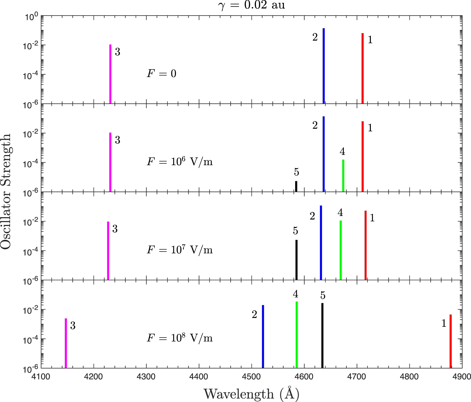
Figure 4. Same as Figure 3, but for γ = 0.2 au.
Download figure:
Standard image High-resolution image
To check the validity of the current approach in calculations of spectral lines related to atomic states in the n = 4 manifold, our spectral data for 10 Balmer β transitions of hydrogen in parallel fields are compared to those from the discretization method (Fassbinder & Schweizer 1996b) in Table 32. A finite nuclear mass is taken into account through a scaling transformation formulated by Pavlov-Verevkin & Zhilinskii (1980), and we took electric field strengths of F = 0, 107, and 108 V m−1, and magnetic field strengths corresponding to the values of Fassbinder & Schweizer (1996b). Good agreement can be observed between our results and theirs, except for the  transition at F = 0, 107, and 108 V m−1. The wavelengths for this transition from the two calculations differ by about 5 Å for these three electric field strengths. It is easily seen from Table 17 that for this transition, the current approach reproduces the wavelengths and oscillator strengths predicted by the finite-basis-set method, and thus we are confident that our results are more accurate than those from the discretization method. Furthermore, Fassbinder & Schweizer (1996b) gave the wavelength and oscillator strength for transition
  at F = 108 V m−1. Our calculation shows that the energy level of the atomic state
  at γ = 0.154 au and F = 108 V m−1 is higher than the classical saddle point
  . The ionization rate of such a state is definitely big, and hence we do not think that it is appropriate to provide its spectral data with the current approach.
Table 32. Comparison of Wavelengths in Angstroms and Oscillator Strengths for 10 Balmer β Spectral Lines from Our Approach and Those from the Discretization Method
| F = 0 V m−1 | F = 107 V m−1 | F = 108 V m−1 | |||||||||||
|---|---|---|---|---|---|---|---|---|---|---|---|---|---|
| Transition | γ (au) | Present | FS | γ (au) | Present | FS | γ (au) | Present | FS | ||||

| 0.1820 | 3760.8 | 3759.3 | 0.1820 | 3760.6 | 3759.1 | 0.0068 | 4871.3 | 4871.2 | ||||
| 2.881(−2) | 0.0289 | 2.837(−2) | 0.0285 | 1.065(−1) | 0.1065 | ||||||||

| 0.0054 | 4930.6 | 4930.5 | 0.0056 | 4929.6 | 4929.5 | 0.0066 | 4893.2 | 4893.1 | ||||
| 2.251(−1) | 0.2251 | 2.196 (−1) | 0.2195 | 1.478(−1) | 0.1477 | ||||||||

| 0.0092 | 4970.7 | 4970.6 | 0.0094 | 4968.5 | 4968.4 | 0.0068 | 4918.7 | 4918.6 | ||||
| 1.126(−1) | 0.1126 | 1.006(−1) | 0.1006 | 3.511(−2) | 0.0354 | ||||||||

| 0.4240 | 4612.9 | 4607.9 | 0.4240 | 4613.1 | 4608.0 | 0.4240 | 4623.4 | 4618.3 | ||||
| 1.554(−2) | 0.0156 | 1.553(−2) | 0.0156 | 1.431(−2) | 0.0144 | ||||||||

| 0.1340 | 4123.8 | 4123.9 | 0.1340 | 4123.2 | 4123.3 | 0.1540 | 4078.2 | 4078.2 | ||||
| 1.477(−1) | 0.1476 | 1.468(−1) | 0.1468 | 9.786(−2) | 0.0978 | ||||||||

| 0.1460 | 3638.6 | 3637.2 | 0.1460 | 3637.2 | 3635.5 | 0.1540 | ⋯ | 3763.1 | ||||
| 5.710(−2) | 0.0574 | 5.462(−2) | 0.0547 | ⋯ | 0.0016 | ||||||||

| 0.0044 | 4918.4 | 4918.4 | 0.0046 | 4914.3 | 4914.3 | 0.0068 | 4811.1 | 4810.9 | ||||
| 0 | 0 | 1.146(−2) | 0.0113 | 2.061(−5) | 0.0000 | ||||||||

| 0.0106 | 4981.4 | 4981.3 | 0.0106 | 4981.1 | 4981.0 | 0.0070 | 4981.7 | 4981.6 | ||||
| 0 | 0 | 5.544(−3) | 0.0055 | 3.632(−3) | 0.0037 | ||||||||

| 0.0124 | 5005.6 | 5005.4 | 0.0124 | 5005.9 | 5005.8 | 0.0100 | 5037.7 | 5037.6 | ||||
| 0 | 0 | 4.621(−4) | 0.0005 | 4.677(−2) | 0.0469 | ||||||||

| 0.0184 | 5067.6 | 5067.4 | 0.0184 | 5068.2 | 5067.9 | 0.0160 | 5114.7 | 5114.5 | ||||
| 0 | 0 | 1.142(−3) | 0.0011 | 4.516(−2) | 0.0452 | ||||||||
Notes. The wavelength and oscillator strength are listed in the upper and lower rows, respectively, for each transition. Three values of electric field strengths of F = 0, 107, and 108 V m−1 were selected, and the magnetic field strengths we took correspond to the values of Fassbinder & Schweizer (1996b). Our results are denoted by "Present," and those of Fassbinder & Schweizer (1996b) by "FS."
Download table as: ASCIITypeset image
4. Summary and Outlook
A two-dimensional B-spline approach has been applied to computations of hydrogen atomic states in the n = 1 and 4 manifolds in the presence of parallel magnetic and electric fields. The influence of electric fields on hydrogen atomic states in white-dwarf-strength magnetic fields has been studied. A strong electric field is found to be able to remarkably change the probability density distributions of atomic states in the n = 4 manifold, and the size of the influence is related to atomic states as well as to magnetic fields. For a given atomic state, its probability density distribution may be primarily located under or above the z = 0 plane, dependent on magnetic and electric field strengths. The current atomic structure data for the n = 1 and 4 manifold states and those for the n = 2 and 3 manifold states previously obtained in Zhao & Liu (2021) were used to calculate Lyman β, γ, and Balmer β spectral lines in parallel fields. The wavelengths and oscillator strengths for a total of 31 transitions are presented as a function of magnetic and electric fields ranging, respectively, from 23.5 to 2350 MG and from 0 to 108 V m−1. We compared our wavelengths and oscillator strengths for the 15 dipole-allowed transitions in a pure magnetic field with those from the finite-basis-set method (Zhao & Liu 2019). Excellent agreement is seen for all 15 dipole-allowed transitions over the entire range of magnetic fields. This confirms the reliability of the two-dimensional B-spline approach in the computations of Lyman β, γ, and Balmer β lines of hydrogen atoms in the presence of parallel fields.
The influence of electric fields on Balmer β lines of magnetized hydrogen atoms has been illustrated. Zeeman spectral lines may be blue- or redshifted with increasing electric fields, dependent on the transitions and magnetic fields. Furthermore, Lyman β and γ spectral lines are found to lie in the ultraviolet region, while the Balmer β lines lie in the ultraviolet and visible-light regions, in the scope of field strengths we are concerned with. To check the validity of the current approach, we compared spectral data for 10 Balmer β transitions of hydrogen in parallel fields to those from the DVR method (Fassbinder & Schweizer 1996b). Good agreement is clearly visible except for the  transition at F = 0, 107, and 108 V m−1. Considering the fact that our spectral data for all the dipole-allowed transitions including this transition in a pure magnetic field is in excellent agreement with those from the other method reported in the literature, we are confident that our results are more accurate than those from the DVR method for the concerned transitions. In particular, the present calculations provide spectral data for more transitions than those given in Fassbinder & Schweizer (1996b).
The atomic spectral data presented in Tables 1–31 are applicable for explaining astronomically observed spectral lines of hydrogen atoms in the atmospheres of magnetic white dwarfs when a strong electric field exists. In particular, the current results are useful to predict additional spectral lines dipole-forbidden in a pure magnetic field. It should be mentioned that the two-dimensional B-spline approach has the potential to be extended to study the problem of multielectronic atoms in magnetic and electric fields of white dwarfs. It should be feasible to handle electron correlation in strong external fields using B-spline functions through configuration interaction. Such work is underway.
This work is supported by the National Natural Science Foundation of China under grant No. 11974087.