


Abstract
Radiative lifetimes of 62 odd-parity levels of Ir i in the energy range between 32513.43 and 58625.10 cm−1 were measured using the time-resolved laser-induced fluorescence technique. The lifetime values obtained are in the range from 3.2 to 345 ns. To our best knowledge, 59 results are reported for the first time. These are compared to computed data deduced from a pseudo-relativistic Hartree–Fock model including core-polarization contributions. From the combination of the experimental lifetime measurements and branching fraction calculations, a new set of transition probabilities and oscillator strengths is derived for 134 Ir i spectral lines of astrophysical interest in the wavelength region from 205 to 418 nm.
Export citation and abstract BibTeX RIS
1. Introduction
Atomic radiative parameters such as oscillator strengths and transition probabilities are very important in astrophysics, plasma diagnostics, analytical chemistry, etc. In astrophysics, the accuracy of stellar chemical abundances largely depends on the adequacy and accuracy of atomic radiative and structure data. For neutral iridium (Ir i, Z = 77), there are two stable isotopes, 191Ir and 193Ir, with relative abundances of 37.3% and 62.7% on the earth and a common nuclear spin of 3/2. Its ionization limit was estimated to be 72323.9 cm−1 (Colarusso et al. 1997). Ir abundances in stars are of great significance not only in radioactive cosmochronology, but also in the structure and nucleosynthetic evolution of supernovae originating from the first stellar generation (Ivarsson et al. 2003).
Ramanujam & Andersen (1978) reported the lifetimes of z6D°9/2 and z6F°7/2,11/2 levels using the beam-sputtering technique. Gough et al. (1983) derived oscillator strengths for 27 transitions in Ir i by combination of the lifetimes of 25 odd-parity levels obtained by the technique of laser-excited fluorescence from sputtered metal vapor and the branching fractions (BFs) by a hollow cathode lamp. Ivarsson et al. (2003) used the time-resolved laser-induced fluorescence (TR-LIF) technique to measure the lifetime of 5d76p z6F°11/2 (28452.32 cm−1) and derived four transition probabilities for two levels by combination with BFs from Fourier transform spectroscopic measurement. Xu et al. (2007) measured lifetimes of nine odd-parity Ir i levels and four odd-parity Ir ii levels using the TR-LIF method and performed corresponding calculations.
As far as we know, the experimental lifetimes of a total of 29 levels in the energy range 26307.49–41118.75 cm−1 in Ir i have been published so far. However, the lifetimes of high-lying levels above 42,000 cm−1 are still unknown. In the present work, we measured the lifetimes for 62 Ir i levels, including 56 levels above 42,000 cm−1, with the TR-LIF technique. These new data were combined with BFs obtained from pseudo-relativistic Hartree–Fock calculations, including core-polarization effects, to deduce semi-empirical transition probabilities and oscillator strengths for 134 Ir i spectral lines involving upper levels ranging from 32513.43 to 49823.54 cm−1.
2. Experimental Setup
The TR-LIF method for radiative lifetime measurements has been fully proven to be very reliable and has been used by many researchers over the past few years (see e.g., Ivarsson et al. 2004; Xu et al. 2007; Den Hartog et al. 2011). The experimental setup used for lifetime measurements in the present work is the same as that recently used by Tian et al. (2016), so only a brief description is given here.
A 532 nm Q-switched Nd:YAG laser with 8 ns pulse duration, 10 Hz repetition rate, and pulse energy of 5–10 mJ was used as an ablation beam to generate Ir laser plasma. A dye laser (Sirah Cobra-stretch) using DCM or Rhodamine 6G dyes, which was pumped by another Nd:YAG laser with the same performance parameters as the former, except for pulse energy, produced a tunable laser at 604–658 nm or 558–588 nm. In order to achieve excitations of higher lying levels, this dye laser needed to be converted into the second or the third harmonic lights through one or two β-barium borate (BBO) type-I crystals, and sometimes the converted harmonic lights were extended as different orders of Stokes and anti-Stokes components by stimulated Raman scattering in a H2 gas cell. The excitation wavelength range for the levels studied in this paper is 204.404–381.832 nm. The ablation laser was focused vertically on the Ir target in the vacuum chamber, where the excitation light passed horizontally through the Ir plasma at a distance of about 8 mm above the target to excite a level of interest. The laser-induced fluorescence from an excited level was collected by a fused silica lens into a grating monochromator and detected by a photomultiplier tube (PMT, Hamamatsu R3896). A 2.5 GHz digital oscilloscope (Tektronix DPO7254) registered and averaged the transient signals from the PMT. A digital delay generator (SRS Model 535) was used to change the delay time between the excitation and ablation pulses. In this work, the lifetime measurements were performed at the delay times from 4 to 45 μs. In order to wipe off Zeeman quantum beats induced by the Earth's magnetic field, a 100 G produced by a pair of Helmholtz coils in horizontal direction was employed to produce high-frequency Zeeman beats, which were out of the detection range of the PMT.
3. Lifetime Measurements
In the measurements, the single-step excitation scheme was employed. The target levels were populated from the ground state or some metastable states like those listed in Table 3. To ensure that only the studied level was excited, the excitation wavelength was carefully chosen from available excitation paths and monitored by a wavemeter (HighFinesse WS6). Moreover, the excited level under study was confirmed by verifying that the observed fluorescence wavelengths were related to this level and their decay behaviors were the same.
All possible systematic effects influencing lifetime results were carefully checked, such as the radiation trapping, the collision deexcitation, and the flight-out-of-view effect. These effects can be eliminated by choosing appropriate experimental conditions through changing the excitation laser energy, the entrance slit of the monochromator and its position along the direction of atomic motion, and the delay time of the excitation pulse relative to the ablation one. More details on the elimination of systematic effects were described in our previous paper (Feng et al. 2011). In order to achieve a good signal-to-noise ratio in the time-resolved fluorescence decay curve, fluorescence signals induced by excitations of over 1000 pulses were acquired and averaged for each decay curve. For each level, more than 10 curves were registered under different experimental conditions, and the level's lifetime is the average of the lifetime values from these curves. Each curve gave two lifetime values. In an exponential fit, the two values were determined with two starting points of fit, respectively. One was a position with the intensity as strong as possible and out of the influence of stray light of the excitation laser, and the other was at half of the intensity of the former point. When using a convolutional fit, two lifetime values were evaluated by means of two excitation-pulse shapes recorded respectively before and after the fluorescence curve registration. The two lifetime values from a decay curve are in good agreement, and their mean value and its deviation from the two values were taken as the lifetime revealed by this curve and its systematic error, respectively. The uncertainty of the final lifetime result for a level is the standard deviations composited from the systematic errors and the statistical errors of different curve measurements.
From experience, when the lifetime value is shorter than 5 times the excitation-pulse width, a convolution fit to the fluorescence decay curve by combining the recorded excitation pulse with an exponential function is necessary for extracting more reliable lifetime value from the decay curve (Li et al. 1999). A typical decay curve observed at 237.040 nm from the 52051.75 to 9877.54 cm−1 levels and fitted by convolution of a excitation-pulse shape and an exponential with 13.5 ns decay constant is shown in Figure 1. For the decay curves of longer lifetimes, exponential fits to the portions where the exciting pulse and its stray light ceased can give accurate decay constants. A typical decay curve observed at 351.594 nm from the 35540.34 to 7106.61 cm−1 levels fitted by an exponential function, giving rise to a lifetime value of 281 ns, is shown in Figure 2. It can be seen from Figures 1 and 2 that the fit curves are in good agreement with the measured fluorescence curves, which benefit from the latter having a good signal-to-noise ratio. The lifetime results measured in the present work are shown in Table 3.
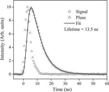
Figure 1. Convolution fitting to a typical fluorescence decay curve of the 52051.75 cm−1 level of Ir i from using a excitation pulse and an exponential function.
Download figure:
Standard image High-resolution image
Figure 2. Exponential fitting to a typical fluorescence decay curve of the 35540.34 cm−1 level of Ir i.
Download figure:
Standard image High-resolution image4. Theoretical Calculations
The theoretical approach used in the present work for computing the radiative parameters in Ir i was the pseudo-relativistic Hartree–Fork (HFR) method of Cowan (1981) modified for taking core-polarization effects into account (HFR+CPOL), as described by Quinet et al. (1999, 2002). Since we considered the same model as the one used in our previous theoretical study of the iridium atom (Xu et al. 2007), just including more transitions in the calculations, only a brief summary is provided here. Twelve even-parity and nine odd-parity configurations were explicitly included in the calculations, namely 5d76s2, 5d76p2, 5d76d2, 5d76s7s, 5d76s6d, 5d66s27s, 5d66s26d, 5d66s6p2, 5d86s, 5d87s, 5d86d, 5d9, and 5d76s6p, 5d76s7p, 5d76s5f, 5d76s6f, 5d66s26p, 5d86p, 5d87p, 5d85f, 5d86f, respectively. The core-polarization effects were estimated using the dipole polarizability reported by Fraga et al. (1976) for an Ir iv ionic core, i.e., αd = 6.48 a03, and a cutoff radius rc = 1.60 a0, corresponding to the expectation value of <r> for the outermost core orbital (5d), as obtained with the HFR method. Moreover, a semi-empirical fitting procedure was applied to the radial parameters related to the 5d76s2, 5d86s, 5d9, 5d76s6p, 5d66s26p, and 5d86p configurations. The details of this semi-empirical process can be found in Xu et al. (2007). It is important to note that the energy levels above 50,000 cm−1 were not included in the fit because many of them were found to be strongly mixed with unknown levels, which made very doubtful the correspondence between the calculated energies and the available experimental values. For this reason, our HFR+CPOL calculations of the atomic structure and radiative parameters in Ir i were limited to the energy levels situated below 50,000 cm−1. The energy levels computed in our work are compared to the available experimental values in Tables 1 and 2 for even and odd parities, respectively. As seen from these tables, a good agreement is obtained between both sets of results, the average deviations being found to be equal to 59 cm−1 (even parity) and 112 cm−1 (odd parity). We can also note that the levels considered in the present study are extremely mixed, in particular for the odd parity for which very strong intermediate coupling and configuration interaction among 5d86p, 5d76s6p, and 5d66s26p are observed, as shown in Table 2. This HFR+CPOL approach was then used to compute the radiative decay rates for the transitions depopulating the Ir i odd energy levels located below 50,000 cm−1. All the line strengths were calculated in the length form.
Table 1. Calculated Energy Levels Compared to Experimentally Known Values for Even Parity in Ir i
| Eexpa | Ecalcb | ΔE | J | LS Compositionb,c |
|---|---|---|---|---|
| (cm−1) | (cm−1) | (cm−1) | (%) | |
| 0.00 | −51 | 51 | 9/2 | 80 5d76s2 4F + 13 5d76s2 2G |
| 2834.98 | 2833 | 2 | 9/2 | 94 5d8(3F)6s 4F |
| 4078.94 | 4153 | −74 | 3/2 | 32 5d76s2 2P + 16 5d8(3P)6s 2P + 13 5d8(1D)6s 2D |
| 5784.62 | 5842 | −57 | 5/2 | 23 5d8(1D)6s 2D + 21 5d76s2 4F + 8 5d9 2D |
| 6323.91 | 6130 | 194 | 7/2 | 54 5d8(3F)6s 4F + 26 5d8(3F)6s 2F |
| 7106.61 | 7055 | 52 | 7/2 | 79 5d76s2 4F + 11 5d8(3F)6s 4F |
| 9877.54 | 9893 | −15 | 5/2 | 32 5d76s2 4F + 24 5d8(3F)6s 4F + 19 5d8(3P)6s 4P |
| 10578.68 | 10697 | −118 | 3/2 | 22 5d8(3F)6s 4F + 22 5d76s2 4P + 19 5d8(1D)6s 2D |
| 11831.09 | 11893 | −62 | 3/2 | 53 5d76s2 4F + 19 5d8(3F)6s 4F + 10 5d8(1D)6s 2D |
| 12218.47 | 12301 | −83 | 5/2 | 58 5d8(3F)6s 4F + 16 5d8(3P)6s 4P + 12 5d8(3F)6s 2F |
| 12505.68 | 12467 | 39 | 1/2 | 45 5d76s2 2P + 28 5d8(3P)6s 2P + 22 5d76s2 4P |
| 12951.67 | 13071 | −119 | 5/2 | 69 5d76s2 4P + 17 5d76s2 4F |
| 13087.90 | 13132 | −44 | 7/2 | 58 5d8(3F)6s 2F + 32 5d8(3F)6s 4F |
| 13939.80 | 13900 | 40 | 9/2 | 54 5d76s2 2G + 20 5d76s2 2H + 13 5d76s2 4F |
| 16103.32 | 16098 | 5 | 5/2 | 40 5d8(3P)6s 4P + 5d9 2D + 12 5d8(3F)6s 2F |
| 16565.35 | 16553 | 12 | 3/2 | 60 5d8(3P)6s 4P + 23 5d8(3F)6s 4F |
| 16681.20 | 16693 | −12 | 1/2 | 87 5d8(3P)6s 4P + 8 5d8(1S)6s 2S |
| 17779.24 | 17772 | 7 | 7/2 | 58 5d76s2 2G + 29 5d8(1G)6s 2G + 6 5d76s2 2F |
| 18547.04 | 18539 | 8 | 3/2 | 34 5d76s2 4P + 29 5d8(3P)6s 4P + 13 5d8(3P)6s 2P |
| 19060.62 | 19149 | −88 | 5/2 | 43 5d8(3F)6s 2F + 30 5d9 2D + 12 5d76s2 2F |
| 19593.25 | 19541 | 53 | 11/2 | 95 5d76s2 2H |
| 20236.70 | 20135 | 102 | 1/2 | 68 5d76s2 4P + 20 5d8(3P)6s 2P |
| 22110.24 | 22028 | 82 | 3/2 | 25 5d8(1D)6s 2D + 21 5d9 2D + 18 5d8(3F)6s 4F |
| 23310.36 | 23218 | 92 | 5/2 | 38 5d76s2 2D + 34 5d9 2D + 7 5d8(1D)6s 2D |
| 23505.91 | 23509 | −3 | 9/2 | 66 5d8(1G)6s 2G + 29 5d76s2 2H |
| 26229.48 | 26252 | −23 | 3/2 | 43 5d76s2 2D + 26 5d8(3P)6s 2P + 13 5d76s2 4F |
| 26365.16 | 26330 | 35 | 7/2 | 63 5d8(1G)6s 2G + 25 5d76s2 2G + 6 5d8(3F)6s 2F |
| 26404.17 | 26293 | 111 | 5/2 | 29 5d8(1D)6s 2D + 27 5d76s2 2F + 15 5d76s2 2D |
| 27913.84 | 28076 | −162 | 9/2 | 46 5d76s2 2H + 28 5d76s2 2G + 20 5d8(1G)6s 2G |
| 27970.05 | 27994 | −24 | 3/2 | 56 5d9 2D + 17 5d8(1D)6s 2D + 9 5d76s2 2D |
Notes.
aFrom Kramida et al. (2018). bThis work. cOnly the first three eigenvector components are given, provided they are greater than or equal to 5%.Download table as: ASCIITypeset image
Table 2. Calculated Energy Levels Compared to Experimentally Known Values for Odd Parity in Ir i up to 50,000 cm−1
| Eexpa | Ecalcb | ΔE | J | LS Compositionb,c |
|---|---|---|---|---|
| (cm−1) | (cm−1) | (cm−1) | (%) | |
| 26307.50 | 26600 | −293 | 9/2 | 52 5d7(4F)6s6p 6D + 23 5d7(4F)6s6p 6F + 8 5d7(2G)6s6p 4F |
| 28452.32 | 28290 | 162 | 11/2 | 63 5d7(4F)6s6p 6F + 19 5d7(4F)6s6p 6G + 7 5d7(4F)6s6p 4G |
| 30529.66 | 30703 | −173 | 7/2 | 37 5d7(4F)6s6p 6D + 28 5d7(4F)6s6p 6F + 6 5d7(2G)6s6p 4F |
| 32463.58 | 32524 | −60 | 3/2 | 24 5d7(2P)6s6p 4P + 9 5d8(3P)6p 4P + 8 5d7(4P)6s6p 6D |
| 32513.43 | 32372 | 141 | 9/2 | 27 5d7(4F)6s6p 6G + 23 5d7(4F)6s6p 6F + 18 5d7(4F)6s6p 6D |
| 32830.78 | 32892 | −61 | 13/2 | 88 5d7(4F)6s6p 6G + 11 5d7(2G)6s6p 4H |
| 33064.83 | 32969 | 96 | 5/2 | 16 5d7(2P)6s6p 4P + 13 5d7(4P)6s6p 6S + 11 5d7(2P)6s6p 4D |
| 33874.43 | 33960 | −86 | 7/2 | 38 5d8(3F)6p 4D + 95d7(4F)6s6p 4D + 8 5d7(4F)6s6p 6F |
| 34180.48 | 34063 | 117 | 11/2 | 28 5d7(4F)6s6p 6G + 25 5d7(4F)6s6p 6F + 23 5d7(4F)6s6p 4G |
| 34919.83 | 34959 | −39 | 5/2 | 45 5d7(4F)6s6p 6F + 12 5d7(4F)6s6p 6D |
| 35080.80 | 35031 | 50 | 9/2 | 16 5d8(3F)6p 4F + 14 5d7(4F)6s6p 4F + 9 5d7(4F)6s6p 6F |
| 35410.63 | 35191 | 220 | 7/2 | 21 5d7(4F)6s6p 6G + 14 5d7(4F)6s6p 6F + 11 5d7(4F)6s6p 6D |
| 35540.34 | 35600 | −60 | 5/2 | 23 5d7(4P)6s6p 6S + 15 5d7(4F)6s6p 6D + 10 5d7(4P)6s6p 6D |
| 35647.94 | 35629 | 19 | 1/2 | 20 5d7(2P)6s6p 4P + 20 5d7(4F)6s6p 6F + 10 5d7(2D)6s6p 4D |
| 36390.15 | 36436 | −46 | 3/2 | 51 5d7(4F)6s6p 6F + 7 5d7(2D)6s6p 4D + 5 5d7(4F)6s6p 6D |
| 37446.13 | 37408 | 38 | 5/2 | 38 5d7(4F)6s6p 6G + 19 5d7(4P)6s6p 6S + 9 5d7(4F)6s6p 6D |
| 37515.31 | 37516 | −1 | 7/2 | 17 5d7(4F)6s6p 6G + 15 5d7(2P)6s6p 4D + 12 5d7(4F)6s6p 4D |
| 37692.75 | 37580 | 113 | 3/2 | 25 5d7(4F)6s6p 6G + 13 5d7(2P)6s6p 4D + 12 5d7(2D)6s6p 4F |
| 37871.69 | 37838 | 34 | 9/2 | 21 5d8(3F)6p 4F + 21 5d7(4F)6s6p 4F + 18 5d7(4F)6s6p 6F |
| 38120.94 | 38082 | 39 | 1/2 | 35 5d7(4F)6s6p 6F + 8 5d7(2P)6s6p 4P + 7 5d7(4P)6s6p 6D |
| 38158.24 | 38182 | −24 | 7/2 | 17 5d7(4F)6s6p 6G + 14 5d7(4F)6s6p 4F + 9 5d6(5D)6s26p 6D |
| 38229.75 | 38255 | −25 | 9/2 | 29 5d8(3F)6p 2G + 19 5d8(3F)6p 4G + 15 5d7(4F)6s6p 6G |
| 38358.13 | 38370 | −12 | 5/2 | 22 5d7(4P)6s6p 6S + 10 5d8(3F)6p 4D + 10 5d7(4F)6s6p 6G |
| 38484.74 | 38582 | −97 | 3/2 | 32 5d7(4F)6s6p 6D + 18 5d7(4P)6s6p 6D + 16 5d7(4F)6s6p 6G |
| 38568.05 | 38537 | 31 | 7/2 | 13 5d7(4F)6s6p 4D + 10 5d7(4F)6s6p 6D + 9 5d7(4F)6s6p 4F |
| 39289.28 | 39384 | −95 | 1/2 | 15 5d7(4F)6s6p 6D + 15 5d7(4P)6s6p 6D + 10 5d8(1D)6p 2P |
| 39324.57 | 39312 | 13 | 5/2 | 11 5d7(4F)6s6p 6D + 9 5d8(1D)6p 2F + 8 5d7(4P)6s6p 6D |
| 39805.97 | 39864 | −58 | 5/2 | 16 5d8(3F)6p 4D + 8 5d7(2P)6s6p 4P + 5 5d7(4F)6s6p 6F |
| 39940.27 | 39821 | 119 | 11/2 | 36 5d8(3F)6p 4G + 29 5d7(4F)6s6p 6G + 18 5d7(4F)6s6p 4G |
| 40291.19 | 40343 | −52 | 7/2 | 15 5d8(3F)6p 2F + 13 5d8(3F)6p 4F |
| 40389.83 | 40270 | 120 | 9/2 | 22 5d7(4F)6s6p 6G + 18 5d7(4F)6s6p 4F |
| 40524.73 | 40640 | −115 | 3/2 | 23 5d7(4F)6s6p 6G + 11 5d7(2P)6s6p 4D + 9 5d6(5D)6s26p 6D |
| 40710.78 | 40766 | −55 | 7/2 | 27 5d7(4P)6s6p 6D + 14 5d6(5D)6s26p 6D |
| 41118.71 | 41076 | 43 | 9/2 | 27 5d6(5D)6s26p 6D + 25 5d7(4P)6s6p 6D + 6 5d7(4F)6s6p 4F |
| 41210.33 | 41217 | −7 | 1/2 | 32 5d7(4F)6s6p 6D + 21 5d6(5D)6s26p 6D + 8 5d7(2P)6s6p 4D |
| 41522.22 | 41640 | −118 | 5/2 | 17 5d7(4P)6s6p 6D + 11 5d6(5D)6s26p 6D + 8 5d8(3F)6p 4D |
| 42014.44 | 42099 | −85 | 1/2 | 29 5d7(2P)6s6p 4D + 16 5d8(3P)6p 4D + 9 5d7(2P)6s6p 4P |
| 42029.14 | 41896 | 133 | 3/2 | 14 5d8(1D)6p 2D + 9 5d7(4F)6s6p 6F + 7 5d7(2D)6s6p 2D |
| 42131.82 | 42279 | −147 | 11/2 | 36 5d8(3F)6p 4G + 20 5d7(4F)6s6p 4G |
| 42267.86 | 42382 | −114 | 5/2 | 14 5d6(5D)6s26p 6D + 11 5d7(4F)6s6p 4F + 7 5d7(4P)6s6p 6D |
| 42279.28 | 42068 | 211 | 9/2 | 15 5d6(5D)6s26p6D + 14 5d7(4F)6s6p 6F |
| 43071.78 | 43021 | 51 | 5/2 | 8 5d8(3F)6p 4G + 8 5d8(3F)6p 4F + 6 5d8(3F)6p 4D |
| 43176.15 | 42973 | 203 | 7/2 | 20 5d8(3F)6p 4G + 8 5d7(2F)6s6p 4G + 7 5d7(4F)6s6p 4G |
| 43200.89 | 43160 | 41 | 3/2 | 13 5d8(3F)6p 4D + 12 5d7(4F)6s6p 4D + 10 5d7(4F)6s6p 4F |
| 43592.21 | 43487 | 105 | 7/2 | 19 5d7(4P)6s6p 6P + 17 5d6(5D)6s26p 6P + 14 5d7(4F)6s6p 6D |
| 44569.85 | 44474 | 96 | 3/2 | 12 5d7(4P)6s6p 6D + 8 5d7(4P)6s6p 4S |
| 44596.77 | 44567 | 30 | 5/2 | 14 5d7(4P)6s6p 6P + 12 5d8(3F)6p 4F + 8 5d7(2P)6s6p 4D |
| 44642.67 | 44883 | −240 | 7/2 | 15 5d7(4F)6s6p 4D + 13 5d6(5D)6s26p 6D + 10 5d7(2G)6s6p 2G |
| 44652.43 | 44734 | −82 | 9/2 | 21 5d7(4F)6s6p 4G + 8 5d7(2G)6s6p 2H + 7 5d7(4P)6s6p 6D |
| 44785.44 | 44782 | 3 | 3/2 | 16 5d7(4P)6s6p 6D + 9 5d6(5D)6s26p 6D + 8 5d7(4P)6s6p 6P |
| 45111.68 | 45400 | −288 | 7/2 | 13 5d7(4F)6s6p 4G + 12 5d7(4F)6s6p 4G + 11 5d8(3F)6p 4G |
| 45185.95 | 45210 | −24 | 5/2 | 15 5d8(3F)6p 4D + 10 5d7(4F)6s6p 4D + 6 5d8(3F)6p 2F |
| 45259.14 | 45186 | 73 | 3/2 | 13 5d7(4P)6s6p 6P + 12 5d8(3F)6p 4F + 8 5d7(4F)6s6p 4F |
| 45415.26 | 45392 | 23 | 1/2 | 13 5d7(4P)6s6p 6D + 12 5d8(3F)6p 4D |
| 45503.15 | 45760 | −256 | 1/2 | 11 5d7(4P)6s6p 6D + 8 5d7(2P)6s6p 2S + 6 5d8(3P)6p 4P |
| 45570.89 | 45638 | −67 | 5/2 | 11 5d7(4F)6s6p 4G + 9 5d7(4F)6s6p 2D |
| 45895.85 | 46030 | −134 | 7/2 | 28 5d8(3F)6p 2F + 12 5d7(4F)6s6p 4F + 10 5d7(4F)6s6p 2F |
| 45957.33 | 45502 | 455 | 11/2 | 34 5d7(2G)6s6p 4H + 20 5d7(2H)6s6p 4I + 12 5d7(2G)6s6p 4G |
| 46093.84 | 46259 | −165 | 5/2 | 13 5d7(4F)6s6p 4G + 8 5d7(4F)6s6p 4G + 7 5d7(4F)6s6p 2D |
| 46220.32 | 46011 | 209 | 9/2 | 19 5d7(4F)6s6p 4F + 11 5d7(2G)6s6p 4H + 11 5d6(5D)6s26p 4F |
| 46371.64 | 46371 | 1 | 9/2 | 33 5d7(4P)6s6p 6D + 12 5d7(4F)6s6p 4G + 10 5d7(2G)6s6p 4F |
| 46471.84 | 46433 | 39 | 3/2 | 14 5d7(2P)6s6p 2D + 12 5d7(4P)6s6p 4D + 9 5d7(4P)6s6p 4S |
| 46618.13 | 46696 | −78 | 3/2 | 19 5d8(3F)6p 4D + 9 5d7(4F)6s6p4F + 7 5d7(4F)6s6p 4D |
| 46979.02 | 46984 | −5 | 7/2 | 11 5d6(5D)6s26p 4D + 9 5d8(3F)6p 2G + 9 5d8(3F)6p 4F |
| 47011.09 | 47005 | 6 | 5/2 | 15 5d8(3F)6p 4G + 11 5d7(2F)6s6p 4G + 5 5d7(2H)6s6p 4G |
| 47165.12 | 47349 | −184 | 7/2 | 13 5d6(5D)6s26p 6F + 10 5d7(4P)6s6p 4D + 6 5d8(1D)6p 2F |
| 47203.81 | 47141 | 63 | 1/2 | 23 5d6(5D)6s26p 6D + 18 5d7(4P)6s6p 6D + 16 5d7(2P)6s6p 2S |
| 47205.57 | 46930 | 276 | 9/2 | 21 5d7(4F)6s6p 2G + 8 5d7(2H)6s6p 4I + 8 5d7(2G)6s6p 4F |
| 47537.29 | 47608 | −71 | 5/2 | 14 5d6(5D)6s26p 6F + 9 5d6(5D)6s26p 6D |
| 47548.69 | 47685 | −136 | 7/2 | 9 5d7(4F)6s6p 4F + 7 5d7(4P)6s6p 6P + 5 5d7(4F)6s6p 4D |
| 47824.93 | 47744 | 81 | 3/2 | 9 5d7(4P)6s6p 4S + 9 5d6(5D)6s26p 6D |
| 47858.47 | 47889 | −31 | 11/2 | 47 5d6(5D)6s26p 6F + 17 5d7(4F)6s6p 4G + 9 5d6(3F)6s26p 4G |
| 48206.57 | 48468 | −261 | 5/2 | 9 5d7(4F)6s6p 4F + 7 5d8(3P)6p 4P + 6 5d7(4P)6s6p 6D |
| 48299.24 | 48147 | 152 | 9/2 | 23 5d8(3F)6p4G + 9 5d7(2F)6s6p 4G + 8 5d8(3F)6p 2G |
| 48440.83 | 48440 | 1 | 3/2 | 14 5d6(5D)6s26p 6F + 9 5d6(5D)6s26p 6D + 8 5d7(4F)6s6p 2D |
| 48448.65 | 48598 | −149 | 7/2 | 39 5d7(2G)6s6p 4H + 6 5d7(4F)6s6p 2F + 5 5d8(3F)6p 4G |
| 48629.22 | 48690 | −61 | 7/2 | 17 5d7(4F)6s6p 4D + 13 5d6(5D)6s26p 6F + 7 5d6(5D)6s26p 4D |
| 48801.91 | 49027 | −225 | 3/2 | 9 5d7(4F)6s6p 4F + 8 5d8(3F)6p 4F + 7 5d7(4F)6s6p 4D |
| 49146.44 | 49234 | −88 | 5/2 | 11 5d7(4P)6s6p 6P + 8 5d7(4F)6s6p 4D + 9 5d7(4F)6s6p 6D |
| 49158.61 | 49570 | −411 | 9/2 | 21 5d6(5D)6s26p 6D + 12 5d6(5D)6s26p 4F + 11 5d6(5D)6s26p 6F |
| 49342.51 | 49466 | −123 | 3/2 | 19 5d7(4P)6s6p 4S + 12 5d7(4P)6s6p 6P + 6 5d8(3P)6p 4P |
| 49446.25 | 49353 | 93 | 1/2 | 15 5d7(4P)6s6p 4D + 13 5d7(4P)6s6p 4P + 10 5d7(4F)6s6p 4D |
| 49719.17 | 48977 | 742 | 11/2 | 33 5d6(5D)6s26p 6F + 18 5d7(2G)6s6p 4G + 15 5d7(4F)6s6p 4G |
| 49779.37 | 49895 | −116 | 5/2 | 12 5d7(4P)6s6p 4P + 75d8(3P)6p 4D + 6 5d7(4F)6s6p 4D |
| 49823.54 | 49765 | 59 | 7/2 | 11 5d8(3F)6p 2G + 11 5d6(5D)6s26p 6F + 11 5d7(2G)6s6p 4F |
Notes.
aFrom Kramida et al. (2018). bThis work. cOnly the first three eigenvector components are given, provided they are greater than or equal to 5%.5. Results and Discussion
The lifetimes measured in the present work for 62 odd-parity levels of Ir i in the region of 32513.43–58625.10 cm−1 are listed in Table 3. Among them, three levels were also studied in the literature through experiments and calculations, thus their previous results are presented for comparison. For the three levels previously reported, it is seen that our results are in rather good agreement with the values measured by Gough et al. (1983) and Xu et al. (2007) using the TR-LIF technique. For the 33874.43 cm−1 level, the result reported by Ramanujam & Andersen (1978) is 34 ± 3 ns, which shows a slightly larger difference with our value of 28.4 ± 0.6 ns and the other two results in the literature. Considering that the former was measured by the beam-sputtering excitation method, which might involve a cascade population for the studied level and hence prolonging its decay time if cascade correction is not performed well, it is reasonable to believe that our result is more reliable.
Table 3. Measured and Calculated Lifetimes for Ir i Levels and Comparison with Previous Results
| Upper Levela | Lower Levela | λExc. | λObs. | Lifetime (ns) | |||||
|---|---|---|---|---|---|---|---|---|---|
| Assignment | E (cm−1) | Assignment | E (cm−1) | (nm) | (nm) | Experiment | Calculation | ||
| This work | Previous | This work | Previous | ||||||
| 5d76s(5F)6p z 6F°9/2 | 32513.43 | 5d76s2 a 4F9/2 | 0 | 307.565 | 381.832 | 345(11) | 335(10)b | 430 | 303c |
| 430c | |||||||||
| 5d76s(5F)6p z 6F°7/2 | 33874.43 | 5d8(3F)6s b 4F9/2 | 2834.98 | 322.171 | 362.97 | 28.4(6) | 27.5(10)b | 21.2 | 15.9c |
| 29.6(20)c | 21.2c | ||||||||
| 34(3)d | |||||||||
| 5d76s(5F)6p z 6G°5/2 | 35540.34 | 5d76s2 a 4F3/2 | 4078.94 | 317.85 | 351.695 | 281(15) | 205 | ||
| 5d76s(5F)6p z 4D°5/2 | 37446.13 | 5d76s2 a 4F5/2 | 5784.62 | 315.841 | 362.732 | 194(15) | 180(10)b | 128 | 94.0c |
| 128c | |||||||||
| 4052°3/2 | 40524.73 | 5d76s2 a 4F5/2 | 5784.62 | 287.852 | 356.9 | 20.4(14) | 43.1 | ||
| 4152°5/2 | 41522.22 | 5d8(3F)6s b 4F5/2 | 9877.54 | 316.009 | 267.071 | 16.8(5) | 19.6 | ||
| 4226°5/2 | 42267.86 | 5d8(3F)6s b 4F5/2 | 9877.54 | 308.734 | 261.856 | 23.3(13) | 28.7 | ||
| 4227°9/2 | 42279.28 | 5d8(3F)6s b 4F7/2 | 7106.61 | 284.312 | 253.522 | 74.0(27) | 57.7 | ||
| 4317°7/2 | 43176.15 | 5d76s2 a 4F9/2 | 0 | 231.609 | 300.313 | 19.7(9) | 26.7 | ||
| 4359°7/2 | 43529.21 | 5d76s2 a 4F9/2 | 0 | 229.399 | 264.497 | 53.2(56) | 50.4 | ||
| 4459°5/2 | 44596.77 | 5d8(3F)6s b 4F5/2 | 9877.54 | 288.025 | 356.743 | 17.5(14) | 20.5 | ||
| 4464°7/2 | 44642.67 | 5d8(3F)6s a 2F5/2 | 12218.47 | 308.412 | 224.001 | 7.7(5) | 15.6 | ||
| 4465°9/2 | 44652.43 | 5d76s2 a 4F9/2 | 0 | 223.952 | 266.341 | 12.2(8) | 27.5 | ||
| 4478°3/2 | 44785.44 | 5d8(3F)6s b 4F5/2 | 9877.54 | 286.468 | 354.357 | 7.1(4) | 28.0 | ||
| 4511°7/2 | 45111.68 | 5d8(3F)6s b 4F5/2 | 9877.54 | 283.816 | 304.014 | 17.9(8) | 29.0 | ||
| 4518°5/2 | 45185.95 | 5d8(3F)6s a 2F7/2 | 13087.90 | 311.545 | 243.268 | 10.4(3) | 10.0 | ||
| 4525°3/2 | 45259.14 | 5d8(3F)6s b 4F5/2 | 9877.54 | 282.633 | 305.311 | 16.8(5) | 20.2 | ||
| 4557°5/2 | 45570.89 | 5d8(3F)6s b 4F5/2 | 9877.54 | 280.164 | 306.568 | 13.1(4) | 11.7 | ||
| 4589°7/2 | 45895.85 | 5d76s2 a 4F9/2 | 0 | 217.885 | 312.93 | 7.6(2) | 9.8 | ||
| 4622°9/2 | 46220.32 | 5d76s2 a 4F9/2 | 0 | 216.355 | 250.649 | 11.4(6) | 26.1 | ||
| 4637°9/2 | 46371.64 | 5d76s2 a 4F9/2 | 0 | 215.649 | 254.68 | 22.6(8) | 21.1 | ||
| 4716°7/2 | 47165.12 | 5d8(3F)6s b 4F9/2 | 2834.98 | 225.58 | 249.635 | 14.3(8) | 16.8 | ||
| 4720°9/2 | 47205.57 | 5d76s2 a 4F9/2 | 0 | 211.839 | 249.383 | 31.7(11) | 24.8 | ||
| 4754°7/2 | 47548.69 | 5d76s2 a 4F9/2 | 0 | 210.311 | 247.267 | 21.7(7) | 29.8 | ||
| 4785°11/2 | 47858.47 | 5d76s2 a 4F9/2 | 0 | 208.949 | 410.634 | 3.7(3) | 6.5 | ||
| 4820°5/2 | 48206.57 | 5d76s2 b 4P5/2 | 16103.32 | 311.495 | 260.899 | 8.3(7) | 13.8 | ||
| 4844°3/2 | 48440.83 | 5d76s2 a 4F3/2 | 4078.94 | 225.419 | 264.116 | 6.2(2) | 40.7 | ||
| 4844°7/2 | 48448.65 | 5d76s2 a 4F9/2 | 0 | 206.404 | 241.855 | 8.5(3) | 15.3 | ||
| 4862°7/2 | 48629.22 | 5d76s2 a 4F9/2 | 0 | 205.638 | 218.368 | 6.3(3) | 6.6 | ||
| 4977°5/2 | 49779.37 | 5d76s2 a 4F3/2 | 4078.94 | 218.816 | 255.098 | 11.0(6) | 23.5 | ||
| 4982° 7/2 | 49823.54 | 5d8(3F)6s b 4F9/2 | 2834.98 | 212.818 | 250.338 | 16.2(5) | 12.4 | ||
| 5016°5/2 | 50169.88 | 5d76s2 a 4F3/2 | 4078.94 | 216.962 | 252.581 | 10.1(4) | |||
| 5056°3/2 | 50564.12 | 5d76s2 a 4F3/2 | 4078.94 | 215.122 | 245.781 | 9.8(3) | |||
| 5058°7/2 | 50580.39 | 5d8(3F)6s b 4F9/2 | 2834.98 | 209.444 | 230.024 | 8.5(6) | |||
| 5116°3/2 | 51166.54 | 5d76s2 a 4F3/2 | 4078.94 | 212.37 | 246.379 | 27.6(4) | |||
| 5142°5/2 | 51427.15 | 5d76s2 a 4F3/2 | 4078.94 | 211.201 | 252.55 | 11.9(5) | |||
| 5147°9/2 | 51470.74 | 5d8(3F)6s b 4F9/2 | 2834.98 | 205.61 | 225.407 | 7.8(4) | |||
| 5181°5/2 | 51814.75 | 5d76s2 a 4F3/2 | 4078.94 | 209.486 | 238.452 | 15.5(4) | |||
| 5198° 1/2 | 51983.92 | 5d76s2 a 4F3/2 | 4078.94 | 208.747 | 241.515 | 13.6(5) | |||
| 5205°5/2 | 52051.75 | 5d76s2 a 4F3/2 | 4078.94 | 208.451 | 237.112 | 13.5(4) | |||
| 5213°7/2 | 52134.11 | 5d76s2 a 4F5/2 | 5784.62 | 215.752 | 250.528 | 10.2(2) | |||
| 5222°7/2 | 52224.37 | 5d76s2 a 4F5/2 | 5784.62 | 215.333 | 249.963 | 7.1(3) | |||
| 5230°3/2 | 52303.65 | 5d76s2 a 4F3/2 | 4078.94 | 207.363 | 239.665 | 8.2(3) | |||
| 5232°5/2 | 52327.33 | 5d76s2 a 4F3/2 | 4078.94 | 207.261 | 235.572 | 7.9(5) | |||
| 5238° 1/2 | 52388.38 | 5d76s2 a 4F3/2 | 4078.94 | 206.999 | 246.565 | 6.8(4) | |||
| 5260°5/2 | 52605.16 | 5d76s2 a 4F3/2 | 4078.94 | 206.074 | 234.041 | 22.4(9) | |||
| 5280°3/2 | 52806.57 | 5d76s2 a 4F3/2 | 4078.94 | 205.222 | 236.81 | 11.7(9) | |||
| 5355°5/2 | 53552.93 | 5d76s2 a 4F5/2 | 5784.62 | 209.344 | 241.929 | 5.9(4) | |||
| 5364°9/2 | 53642.06 | 5d76s2 a 4F7/2 | 6323.91 | 211.335 | 246.584 | 5.0(3) | |||
| 5368°7/2 | 53686.99 | 5d76s2 a 4F7/2 | 6323.91 | 211.135 | 241.147 | 6.4(3) | |||
| 5411°5/2 | 54119.23 | 5d76s2 a 4F5/2 | 5784.62 | 206.891 | 229.671 | 9.0(5) | |||
| 5414°7/2 | 54140.83 | 5d8(3F)6s b 4F7/2 | 7106.61 | 212.611 | 248.75 | 5.7(3) | |||
| 5426°9/2 | 54263.79 | 5d76s2 a 4F7/2 | 6323.91 | 208.595 | 242.861 | 20.3(7) | |||
| 5456°7/2 | 54566.06 | 5d76s2 a 4F7/2 | 6323.91 | 207.288 | 236.141 | 6.4(4) | |||
| 5463°5/2 | 54639.31 | 5d76s2 a 4F7/2 | 6323.91 | 206.973 | 233.6 | 5.8(4) | |||
| 5466°9/2 | 54667.54 | 5d76s2 a 4F7/2 | 6323.91 | 206.852 | 320.907 | 21.0(17) | |||
| 5471°7/2 | 54711.10 | 5d8(3F)6s b 4F7/2 | 7106.61 | 210.064 | 259.015 | 7.7(5) | |||
| 5489°7/2 | 54894.82 | 5d76s2 a 4F5/2 | 5784.62 | 203.624 | 257.788 | 11.8(6) | |||
| 5503°9/2 | 55035.94 | 5d8(3F)6s b 4F7/2 | 7106.61 | 208.641 | 238.39 | 3.2(3) | |||
| 5769°7/2 | 57697.46 | 5d8(3F)6s b 4F5/2 | 9877.54 | 209.118 | 250.512 | 7.2(4) | |||
| 5811°5/2 | 58117.84 | 5d8(3F)6s b 4F5/2 | 9877.54 | 207.296 | 238.031 | 8.8(3) | |||
| 5862°7/2 | 58625.10 | 5d8(3F)6s b 4F5/2 | 9877.54 | 205.138 | 235.174 | 5.1(3) | |||
Notes. The number in parentheses is the uncertainty in the last one or two digits of the reported result.
aKramida et al. (2018). bGough et al. (1983). cXu et al. (2007). dRamanujam & Anderson (1978).In Table 3, except for the three energy levels with previous results, to our best knowledge the other 59 levels are experimentally measured for the first time. The measured lifetime values are in the range from 3.2 to 345 ns, and their uncertainties are smaller than 10% (except 10.5% for the level at 43529.31 cm−1) and more than half of them are within 5%.
Our HFR+CPOL theoretical lifetimes are also given in Table 3. The general agreement between theory and experiment can be judged as rather satisfactory (within a factor of 2), if we discount the two J = 3/2 levels at 44785.44 and 48440.83 cm−1 for which the calculated lifetimes are respectively a factor of about 4 and 7 longer than the experimental values. It is worth noting that, according to our calculations, most of the highly excited levels considered in the present work were found to be extremely mixed with, on average, a main LS component as low as 20% for all the levels listed in Table 3, and this main component not exceeding even 15% for the levels located between 40,000 and 50,000 cm−1.
Using the theoretical BFs and the experimental lifetimes, we deduced the transition probabilities and oscillator strengths for all the lines depopulating the odd-parity levels below 50,000 cm−1. The results obtained are reported in Table 4. These correspond to 134 Ir i spectral lines appearing in the wavelength range from 205 to 418 nm. Note that concerning the BFs, only the values larger than 0.05 have been retained in the table. To our knowledge, transition probabilities were experimentally measured by Gough et al. (1983) for only two transitions among those considered in the present work. These are found to be in good agreement (within 20%) with our values.
Table 4. Branching Fractions, Transition Probabilities, and Oscillator Strengths Obtained in the Present Work for Highly Excited Levels of Ir i, and Comparison with Previous Results
| Upper Levela | Lower Levela | λair (nm) | BFb | gA(106s−1) | Log(gf ) | |||||||
|---|---|---|---|---|---|---|---|---|---|---|---|---|
| Assign. | E (cm−1) Lifetime (ns) | Assign. | E (cm−1) | This workb | Previous | This workc | Previous | |||||
| Exp. | Exp. | Calc. | ||||||||||
| 5d76s(5F)6p z 6F°9/2 | 32513.43 | 5d76s2 a 4F9/2 | 0.00 | 307.476 | 0.10* | 2.89 (E) | −2.38 (E) | −2.34d | ||||
| τ = 345(11) | 5d8(3F)6s b 4F9/2 | 2834.98 | 336.848 | 0.21 | 6.09 (D+) | −1.98 (D+) | −1.98d | |||||
| 5d76s2 a 4F7/2 | 6323.91 | 381.724 | 0.17 | 4.93 (E) | −1.97 (E) | −1.96d | ||||||
| 5d8(3F)6s b 4F7/2 | 7106.61 | 393.484 | 0.51 | 14.7 (D+) | −1.47 (D+) | −1.45d | ||||||
| 5d76s(5F)6p z 6F°7/2 | 33874.43 | 5d8(3F)6s b 4F9/2 | 2834.98 | 322.078 | 0.80 | 225 (B) | 192.9e | −0.46 (B) | −0.523d | −0.47d | ||
| τ = 28.4(6) | 5d76s2 a 4F7/2 | 6323.91 | 362.867 | 0.06 | 16.9 (E) | 22.7e | −1.48 (E) | −1.35d | −1.51d | |||
| 5d76s(5F)6p z 6G°5/2 | 35540.34 | 5d76s2 a 4F3/2 | 4078.94 | 317.758 | 0.60 | 12.8 (D+) | −1.71 (D+) | |||||
| τ = 281(15) | 5d8(3F)6s b 4F7/2 | 7106.61 | 351.594 | 0.23 | 4.91 (D+) | −2.05 (D+) | ||||||
| 5d76s(5F)6p z 4D°5/2 | 37446.13 | 5d76s2 a 4F3/2 | 4078.94 | 299.609 | 0.44 | 13.6 (D+) | −1.74 (D+) | −1.70d | ||||
| τ = 194(15) | 5d76s2 a 4F5/2 | 5784.62 | 315.750 | 0.11 | 3.40 (E) | −2.29 (E) | −2.28d | |||||
| 5d76s2 a 4F7/2 | 6323.91 | 321.221 | 0.11 | 3.40 (E) | −2.28 (E) | −2.36d | ||||||
| 5d8(3F)6s b 4F5/2 | 9877.54 | 362.629 | 0.22 | 6.80 (D+) | −1.87 (D+) | −1.85d | ||||||
| 5d8(3F)6s b 4F3/2 | 11831.09 | 390.285 | 0.09 | 2.78 (E) | −2.20 (E) | −2.16d | ||||||
| 4052°3/2 | 40524.73 | 5d76s2 a 4F5/2 | 5784.62 | 287.768 | 0.30 | 58.8 (D+) | −1.14 (D+) | |||||
| τ = 20.4(14) | 5d8(3F)6s b 4F5/2 | 9877.54 | 326.200 | 0.15 | 29.4 (E) | −1.33 (E) | ||||||
| 5d8(3P)6s a 2P3/2 | 10578.68 | 333.838 | 0.19 | 37.3 (E) | −1.21 (E) | |||||||
5d8(3P)6s a 2P
|
12505.68 | 356.798 | 0.07 | 13.7 (E) | −1.58 (E) | |||||||
| 5d8(3P)6s a 4P5/2 | 12951.67 | 362.570 | 0.10 | 19.6 (E) | −1.41 (E) | |||||||
| 5d8(3P)6s a 4P3/2 | 16565.35 | 417.255 | 0.14 | 27.4 (E) | −1.14 (E) | |||||||
| 4152°5/2 | 41522.22 | 5d76s2 a 4F3/2 | 4078.94 | 266.992 | 0.16 | 57.1 (E) | −1.21 (E) | |||||
| τ = 16.8(5) | 5d76s2 a 4F5/2 | 5784.62 | 279.735 | 0.24 | 85.7 (D+) | −1.00 (D+) | ||||||
| 5d76s2 a 4F7/2 | 6324.91 | 284.021 | 0.25 | 89.3 (D+) | −0.97 (D+) | |||||||
| 5d8(3F)6s b 4F7/2 | 7106.61 | 290.481 | 0.14 | 50.0 (E) | −1.20 (E) | |||||||
| 5d8(3F)6s b 4F5/2 | 9877.54 | 315.918 | 0.06 | 21.4 (E) | −1.49 (E) | |||||||
| 5d8(3P)6s a 2P3/2 | 10578.68 | 323.076 | 0.11 | 39.3 (E) | −1.21 (E) | |||||||
| 4226°5/2 | 42267.86 | 5d76s2 a 4F3/2 | 4078.94 | 261.778 | 0.50 | 129 (D+) | −0.88 (D+) | |||||
| τ = 23.3(13) | 5d76s2 a 4F7/2 | 6323.91 | 278.129 | 0.33 | 85.0 (D+) | −1.01 (D+) | ||||||
| 5d8(3F)6s b 4F5/2 | 9877.54 | 308.644 | 0.09 | 23.2 (E) | −1.48 (E) | |||||||
| 4227°9/2 | 42279.28 | 5d8(3F)6s b 4F9/2 | 2834.98 | 253.446 | 0.89 | 120 (C+) | −0.94 (C+) | |||||
| τ = 74.0(27) | ||||||||||||
| 4317°7/2 | 43176.15 | 5d76s2 a 4F9/2 | 0.00 | 231.538 | 0.09 | 36.5 (E) | −1.53 (E) | |||||
| τ = 19.7(9) | 5d76s2 a 4F5/2 | 5784.62 | 267.361 | 0.15 | 60.9 (E) | −1.19 (E) | ||||||
| 5d76s2 a 4F7/2 | 6323.91 | 271.274 | 0.14 | 56.8 (E) | −1.20 (E) | |||||||
| 5d8(3F)6s b 4F5/2 | 9877.54 | 300.225 | 0.14 | 56.8 (E) | −1.11 (E) | |||||||
| 5d8(3F)6s a 2F5/2 | 12218.47 | 322.929 | 0.18 | 73.1 (E) | −0.94 (E) | |||||||
| 5d8(3F)6s a 2F7/2 | 13087.90 | 332.260 | 0.20 | 81.2 (D+) | −0.87 (D+) | |||||||
| 4359°7/2 | 43529.21 | 5d8(3F)6s b 4F9/2 | 2834.98 | 245.281 | 0.07 | 9.96 (E) | −2.04 (E) | |||||
| τ = 56.2(56) | 5d76s2 a 4F5/2 | 5784.62 | 264.418 | 0.10 | 14.2 (E) | −1.82 (E) | ||||||
| 5d8(3F)6s b 4F7/2 | 7106.61 | 274.000 | 0.07 | 9.96 (E) | −1.95 (E) | |||||||
| 5d8(3F)6s b 4F5/2 | 9877.54 | 296.520 | 0.05 | 7.12 (E) | −2.02 (E) | |||||||
| 5d8(3F)6s a 2F7/2 | 13087.90 | 327.729 | 0.17 | 24.2 (E) | −1.41 (E) | |||||||
| 5d76s2 a 2G9/2 | 13939.80 | 337.144 | 0.09 | 12.8 (E) | −1.66 (E) | |||||||
| 4459°5/2 | 44596.77 | 5d76s2 a 4F3/2 | 4078.94 | 246.730 | 0.31 | 106 (D+) | −1.01 (D+) | |||||
| τ = 17.5(14) | 5d8(3F)6s b 4F5/2 | 9877.54 | 287.941 | 0.36 | 123 (D+) | −0.82 (D+) | ||||||
| 5d8(3P)6s a 4P5/2 | 12951.67 | 315.914 | 0.09 | 30.9 (E) | −1.34 (E) | |||||||
| 5d8(3F)6s a 2F7/2 | 13087.90 | 317.279 | 0.06 | 20.6 (E) | −1.51 (E) | |||||||
| 4464°7/2 | 44642.67 | 5d8(3F)6s b 4F9/2 | 2834.98 | 239.117 | 0.51 | 530 (D+) | −0.34 (D+) | |||||
| τ = 7.7(5) | 5d8(3F)6s a 2F5/2 | 12218.47 | 308.322 | 0.11 | 114 (E) | −0.79 (E) | ||||||
| 5d8(3P)6s a 4P5/2 | 12951.67 | 315.456 | 0.07 | 72.7 (E) | −0.97 (E) | |||||||
| 5d8(3F)6s a 2F7/2 | 13087.90 | 316.817 | 0.14 | 145 (E) | −0.66 (E) | |||||||
| 4465°9/2 | 44652.43 | 5d76s2 a 4F9/2 | 0.00 | 223.882 | 0.15 | 123 (E) | −1.03 (E) | |||||
| τ = 12.2(8) | 5d8(3F)6s b 4F9/2 | 2834.98 | 239.062 | 0.31 | 254 (D+) | −0.66 (D+) | ||||||
| 5d76s2 a 4F7/2 | 6323.91 | 260.824 | 0.11 | 90.2 (E) | −1.04 (E) | |||||||
| 5d8(3F)6s b 4F7/2 | 7106.61 | 266.262 | 0.34 | 279 (D+) | −0.53 (D+) | |||||||
| 5d8(3F)6s a 2F7/2 | 13087.90 | 316.719 | 0.07 | 57.4 (E) | −1.06 (E) | |||||||
| 4478°3/2 | 44785.44 | 5d8(3F)6s b 4F5/2 | 9877.54 | 286.384 | 0.17 | 95.8 (E) | −0.93 (E) | |||||
| τ = 7.1(4) | 5d8(3F)6s a 2F5/2 | 12218.47 | 306.971 | 0.27 | 152 (D+) | −0.67 (D+) | ||||||
| 5d8(3P)6s a 4P5/2 | 12951.67 | 314.041 | 0.10 | 56.3 (E) | −1.08 (E) | |||||||
| 5d76s2 b 4P5/2 | 16103.32 | 348.549 | 0.14 | 78.9 (E) | −0.84 (E) | |||||||
5d8(3P)6s a 4P
|
16681.20 | 355.716 | 0.15 | 84.5 (E) | −0.79 (E) | |||||||
| 4511°7/2 | 45111.68 | 5d76s2 a 4F5/2 | 5784.62 | 254.202 | 0.07 | 31.3 (E) | −1.51 (E) | |||||
| τ = 17.9(8) | 5d8(3F)6s b 4F7/2 | 7106.61 | 263.051 | 0.08 | 35.8 (E) | −1.43 (E) | ||||||
| 5d8(3F)6s b 4F5/2 | 9877.54 | 283.739 | 0.25 | 112 (D+) | −0.87 (D+) | |||||||
| 5d8(3F)6s a 2F5/2 | 12218.47 | 303.932 | 0.42 | 188 (D+) | −0.58 (D+) | |||||||
| 5d8(3F)6s a 2F7/2 | 13087.90 | 312.180 | 0.07 | 31.3 (E) | −1.34 (E) | |||||||
| 4518°5/2 | 45185.95 | 5d8(3F)6s b 4F7/2 | 7106.61 | 262.532 | 0.51 | 294 (D+) | −0.52 (D+) | |||||
| τ = 10.4(3) | 5d8(3F)6s b 4F3/2 | 11831.09 | 299.719 | 0.07 | 40.4 (E) | −1.26 (E) | ||||||
| 5d8(3F)6s a 2F5/2 | 12218.47 | 303.241 | 0.16 | 92.3 (E) | −0.89 (E) | |||||||
| 5d8(3F)6s a 2F7/2 | 13087.90 | 311.455 | 0.07 | 40.4 (E) | −1.23 (E) | |||||||
| 4525°3/2 | 45259.14 | 5d76s2 a 4F3/2 | 4078.94 | 242.761 | 0.16 | 38.1 (E) | −1.47 (E) | |||||
| τ = 16.8(5) | 5d76s2 a 4F5/2 | 5784.62 | 253.252 | 0.23 | 54.8 (D+) | −1.28 (D+) | ||||||
| 5d8(3F)6s b 4F5/2 | 9877.54 | 282.550 | 0.08 | 19.0 (E) | −1.64 (E) | |||||||
| 5d8(3F)6s b 4F3/2 | 11831.09 | 299.063 | 0.34 | 80.9 (D+) | −0.96 (D+) | |||||||
| 4557°5/2 | 45570.89 | 5d76s2 a 4F3/2 | 4078.94 | 240.938 | 0.63 | 289 (C) | −0.61 (C) | |||||
| τ = 13.1(4) | 5d76s2 a 4F5/2 | 5784.62 | 251.267 | 0.06 | 27.5 (E) | −1.59 (E) | ||||||
| 5d8(3F)6s b 4F5/2 | 9877.54 | 280.081 | 0.15 | 68.7 (E) | −1.10 (E) | |||||||
| 4589°7/2 | 45895.85 | 5d76s2 a 4F9/2 | 0.00 | 217.817 | 0.23 | 242 (D+) | −0.76 (D+) | |||||
| τ = 7.6(2) | 5d8(3F)6s b 4F7/2 | 7106.61 | 257.726 | 0.27 | 284 (D+) | −0.55 (D+) | ||||||
| 5d8(3F)6s a 2F7/2 | 13087.90 | 304.715 | 0.28 | 295 (D+) | −0.39 (D+) | |||||||
| 5d76s2 a 2G9/2 | 13939.80 | 312.839 | 0.11 | 116 (E) | −0.77 (E) | |||||||
| 4622°9/2 | 46220.32 | 5d76s2 a 4F9/2 | 0.00 | 216.287 | 0.36 | 316 (D+) | −0.65 (D+) | |||||
| τ = 11.4(6) | 5d8(3F)6s b 4F9/2 | 2834.98 | 230.422 | 0.28 | 246 (D+) | −0.71 (D+) | ||||||
| 5d76s2 a 4F7/2 | 6323.91 | 250.574 | 0.05 | 43.9 (E) | −1.38 (E) | |||||||
| 5d8(3F)6s a 2F7/2 | 13087.90 | 301.731 | 0.26 | 228 (D+) | −0.51 (D+) | |||||||
| 4637°9/2 | 46371.64 | 5d76s2 a4F9/2 | 0.00 | 215.581 | 0.45 | 199 (D+) | −0.86 (D+) | |||||
| τ = 22.6(8) | 5d8(3F)6s b 4F9/2 | 2834.98 | 229.620 | 0.08 | 35.4 (E) | −1.55 (E) | ||||||
| 5d76s2 a 4F7/2 | 6323.91 | 249.627 | 0.14 | 61.9 (E) | −1.24 (E) | |||||||
| 5d8(3F)6s b 4F7/2 | 7106.61 | 254.604 | 0.20 | 88.5 (D+) | −1.06 (D+) | |||||||
| 5d8(3F)6s a 2F7/2 | 13087.90 | 300.359 | 0.09 | 39.8 (E) | −1.27 (E) | |||||||
| 4716°7/2 | 47165.12 | 5d76s2 a 4F5/2 | 5784.62 | 241.587 | 0.06 | 33.6 (E) | −1.53 (E) | |||||
| τ = 14.3(8) | 5d76s2 a 4F7/2 | 6323.91 | 244.777 | 0.24 | 134 (D+) | −0.92 (D+) | ||||||
| 5d8(3F)6s b 4F7/2 | 7106.61 | 249.560 | 0.11 | 61.5 (E) | −1.24 (E) | |||||||
| 5d8(3F)6s a 2F5/2 | 12218.47 | 286.066 | 0.36 | 201 (D+) | −0.61 (D+) | |||||||
| 5d8(3F)6s a 2F7/2 | 13087.90 | 293.365 | 0.07 | 39.2 (E) | −1.30 (E) | |||||||
| 4720°9/2 | 47205.57 | 5d76s2 a 4F9/2 | 0.00 | 211.772 | 0.09 | 28.4 (E) | −1.72 (E) | |||||
| τ = 31.7(11) | 5d8(3F)6s b 4F9/2 | 2834.98 | 225.305 | 0.05 | 15.8 (E) | −1.92 (E) | ||||||
| 5d76s2 a 4F7/2 | 6323.91 | 244.534 | 0.12 | 37.9 (E) | −1.47 (E) | |||||||
| 5d8(3F)6s b 4F7/2 | 7106.61 | 249.308 | 0.64 | 202 (E) | −0.73 (E) | |||||||
| 5d76s2 a 2G9/2 | 13939.80 | 300.521 | 0.06 | 18.9 (E) | −1.59 (E) | |||||||
| 4754°7/2 | 47548.69 | 5d76s2 a4F9/2 | 0.00 | 210.244 | 0.17 | 62.7 (E) | −1.38 (E) | |||||
| τ = 21.7(7) | 5d8(3F)6s b 4F9/2 | 2834.98 | 223.576 | 0.23 | 84.8 (D+) | −1.20 (D+) | ||||||
| 5d8(3F)6s b 4F5/2 | 9877.54 | 265.376 | 0.07* | 25.8 (E) | −1.56 (E) | |||||||
| 5d8(3F)6s a 2F5/2 | 12218.47 | 282.961 | 0.13 | 47.9 (E) | −1.24 (E) | |||||||
| 5d76s2 b 4P5/2 | 16103.32 | 317.920 | 0.19 | 70.0 (E) | −0.97 (E) | |||||||
| 4785°11/2 | 47858.47 | 5d76s2 a 4F9/2 | 0.00 | 208.883 | 0.89 | 2886 (C+) | 0.28 (C+) | |||||
| τ = 3.7(3) | 5d8(3F)6s b 4F9/2 | 2834.98 | 222.037 | 0.11 | 357 (E) | −0.58 (E) | ||||||
| 4820°5/2 | 48206.57 | 5d76s2 a 4F3/2 | 4078.94 | 226.545 | 0.16 | 116 (E) | −1.05 (E) | |||||
| τ = 8.3(7) | 5d76s2 a 4F7/2 | 6323.91 | 238.689 | 0.30 | 217 (D+) | −0.73 (D+) | ||||||
| 5d8(3F)6s b 4F5/2 | 9877.54 | 260.821 | 0.15 | 108 (E) | −0.96 (E) | |||||||
| 5d8(3P)6s a 2P3/2 | 10578.68 | 265.681 | 0.16 | 116 (E) | −0.91 (E) | |||||||
| 5d8(3P)6s a 4P5/2 | 12951.67 | 283.566 | 0.09* | 65.1 (E) | −1.11 (E) | |||||||
| 5d76s2 b 4P3/2 | 18547.04 | 337.063 | 0.05 | 36.1 (E) | −1.21 (E) | |||||||
| 4844°3/2 | 48440.83 | 5d8(3P)6s a 2P3/2 | 10578.68 | 264.037 | 0.07* | 45.2 (E) | −1.32 (E) | |||||
| τ = 6.2(2) | 5d8(3F)6s b 4F3/2 | 11831.09 | 273.070 | 0.62 | 400 (C) | −0.35 (C) | ||||||
5d8(3P)6s a 2P
|
12505.68 | 278.197 | 0.10 | 64.5 (D) | −1.13 (D) | |||||||
| 4844°7/2 | 48448.65 | 5d76s2 a 4F5/2 | 5784.62 | 234.317 | 0.09 | 84.7 (E) | −1.16 (E) | |||||
| τ = 8.5(3) | 5d76s2 a 4F7/2 | 6323.91 | 237.318 | 0.55 | 517 (D+) | −0.36 (D+) | ||||||
| 5d8(3F)6s b 4F7/2 | 7106.61 | 241.812 | 0.14 | 132 (E) | −0.94 (E) | |||||||
| 5d8(3F)6s a 2F5/2 | 12218.47 | 275.931 | 0.10 | 94.1 (E) | −0.97 (E) | |||||||
| 4862°7/2 | 48629.22 | 5d76s2 a 4F9/2 | 0.00 | 205.572 | 0.06 | 76.2 (E) | −1.32 (E) | |||||
| τ = 6.3(3) | 5d8(3F)6s b 4F9/2 | 2834.98 | 218.300 | 0.45 | 571 (D+) | −0.39 (D+) | ||||||
| 5d76s2 a 4F5/2 | 5784.62 | 233.330 | 0.24 | 305 (D+) | −0.60 (D+) | |||||||
| 5d8(3F)6s b 4F7/2 | 7106.61 | 240.760 | 0.09 | 114 (E) | −1.00 (E) | |||||||
| 5d8(3F)6s b 4F5/2 | 9877.54 | 257.976 | 0.05 | 63.5 (E) | −1.20 (E) | |||||||
| 4977°5/2 | 49779.37 | 5d76s2 a 4F3/2 | 4078.94 | 218.748 | 0.15 | 81.8 (E) | −1.23 (E) | |||||
| τ = 11.0(6) | 5d76s2 a 4F7/2 | 6323.91 | 230.050 | 0.10 | 54.5 (E) | −1.36 (E) | ||||||
| 5d8(3F)6s b 4F7/2 | 7106.61 | 234.270 | 0.18 | 98.2 (E) | −1.09 (E) | |||||||
| 5d8(3P)6s a 2P3/2 | 10578.68 | 255.021 | 0.12 | 65.5 (E) | −1.20 (E) | |||||||
| 5d8(3F)6s a2F7/2 | 13087.90 | 272.462 | 0.16 | 87.3 (E) | −1.01 (E) | |||||||
| 5d8(3P)6s a 4P3/2 | 16565.35 | 300.990 | 0.08 | 43.6 (E) | −1.23 (E) | |||||||
| 5d76s2 b 4P3/2 | 18547.04 | 320.089 | 0.08 | 43.6 (E) | −1.17 (E) | |||||||
| 4982° 7/2 | 49823.54 | 5d76s2 a 4F5/2 | 5784.62 | 227.002 | 0.29 | 143 (D+) | −0.96 (D+) | |||||
| τ = 16.2(5) | 5d76s2 a 4F7/2 | 6323.91 | 229.816 | 0.31 | 153 (D+) | −0.92 (D+) | ||||||
| 5d8(3F)6s b 4F5/2 | 9877.54 | 250.263 | 0.15 | 74.1 (E) | −1.16 (E) | |||||||
| 5d8(1D)6s a2D5/2 | 19060.62 | 324.973 | 0.09 | 44.4 (E) | −1.15 (E) | |||||||
Notes.
aKramida et al. (2018). bCalculated branching fractions with * are characterized by cancellation factors smaller than 0.01 (see text). cgA- and log gf -values obtained in this work were deduced from the combination of HFR+CPOL branching fractions with experimental lifetimes. The estimated uncertainties are given in parentheses. They are indicated by the same letter coding one used in the NIST database (Kramida et al. 2018), i.e., B+ (≤7%), B (≤10%), C+ (≤18%), C (≤25%), D+ (≤40%), D (≤50%), and E (>50%) (see the text). dXu et al. (2007). eGough et al. (1983).The estimated uncertainties of the transition probabilities and oscillator strengths obtained in our work are also reported in Table 4, using the letter coding as the one usually employed in the NIST database (Kramida et al. 2018). They were evaluated as follows. First, an uncertainty was assigned to all our calculated HFR+CPOL BF values by comparing the latter to those deduced from experimental measurements by Gough et al. (1983) and Ivarsson et al. (2003) for some transitions depopulating Ir i levels up to 40,710 cm−1. Such a comparison is reported in Table 7 of Xu et al. (2007) and illustrated in Figure 3 of the present paper where the relative differences (BFcalc–BFexp)/BFcalc are reported against BFcalc. When looking at this figure, one can clearly note a rather regular pattern of increasingly deviating weak branches, the average uncertainties on calculated BF-values being found to be about 10%, for 0.8 < BFcalc < 1.0, 20% for 0.6 < BFcalc < 0.8, 30% for 0.4 < BFcalc < 0.6, 40% for 0.2 < BFcalc < 0.4 and 100% for 0.0 < BFcalc < 0.2. These uncertainties were then combined in quadrature with the experimental lifetime uncertainties derived from our measurements to yield the uncertainties of gA- and gf -values. As a final result, out of the 134 transitions listed in Table 4, 46 have an estimated decay rate accuracy that is better than 50%, which illustrates the fact that many of the highly excited levels considered in the present work are depopulated by quite a number of weak transitions. Moreover, a few transitions reported in Table 4 with an asterisk were found to be affected by strong cancellation effects in our HFR+CPOL calculations. More precisely, for such transitions, the cancellation factor (CF), as defined by Cowan (1981), was estimated to be smaller than 0.01, indicating that the corresponding line strength, and thus the BF or transition probability, might be expected to show a larger percentage uncertainty.

Figure 3. Comparison between the branching fractions calculated in the present work (BFcalc) using the HFR+CPOL approach and the experimental values (BFexp) measured by Gough et al. (1983) and Ivarsson et al. (2003).
Download figure:
Standard image High-resolution image
This work was supported by the Science and Technology Development Planning Project of Jilin Province (Grant No. 20180101239JC). P.P. and P.Q. are respectively Research Associate and Research Director of the Belgian F.R.S.-FNRS, from which financial support is gratefully acknowledged.