


Abstract
We present the results from a complex study of an eclipsing O-type binary (Aa+Ab) with the orbital period of PA = 3.2254367 days that forms part of a higher-order multiple system in a configuration of (A+B)+C. We derived masses of the Aa+Ab binary of M1 = 19.02 ± 0.12 and M2 = 17.50 ± 0.13 M ⊙, the radii of R1 = 7.70 ± 0.05 and R2 = 6.64 ± 0.06 R⊙, and temperatures of T1 = 34,250 ± 500 K and T2 = 33,750 ± 500 K. From the analysis of the radial velocities, we found a spectroscopic orbit of A in the outer A+B system with PA+B = 195.8 days (PA+B/PA ≈ 61). In the O − C analysis, we confirmed this orbit and found another component orbiting the A+B system with PAB+C = 2550 days (PAB+C/PA+B ≈ 13). From the total mass of the inner binary and its outer orbit, we estimated the mass of the third object, MB ≳ 10.7 M⊙. From the light travel time effect fit to the O − C data, we obtained the limit for the mass of the fourth component, MC ≳ 7.3 M⊙. These extra components contribute about 20%–30% (increasing with wavelength) to the total system light. From the comparison of model spectra with the multiband photometry, we derived a distance modulus of 18.59 ± 0.06 mag, a reddening of 0.16 ± 0.02 mag, and an RV of 3.2. This work is part of our ongoing project, which aims to calibrate the surface brightness–color relation for early-type stars.
Export citation and abstract BibTeX RIS

Original content from this work may be used under the terms of the Creative Commons Attribution 4.0 licence. Any further distribution of this work must maintain attribution to the author(s) and the title of the work, journal citation and DOI.
1. Introduction
OGLE LMC-ECL-21568 (henceforth BLMC-03) is located in the region known as the Lucke–Hodge 101 OB association (Lucke & Hodge 1970) or NGC 2074 in the Large Magellanic Cloud (LMC). It is included in photographic, photometric, and spectroscopic studies of the region (e.g., Westerlund 1961; Testor & Niemela 1998) and observed in various photometric surveys of the LMC (e.g., Massey et al. 2002; Zaritsky et al. 2004).
In the first paper of the series by Massey et al. (2002) regarding the program to find eclipsing massive binaries in the LMC, Massey et al. (2012) presented a spectroscopic follow-up of BLMC-03 (under ID [M2002] LMC 172231 from the catalog of Massey et al. 2002) and classified it spectroscopically as O9V+O9.5V. They measured the radial velocities (RVs) of the components and obtained an orbital solution. Combining these data with their new V-band photometry, Massey et al. (2012) provided the first characterization of the system. They found the binary's light and RV curves to be consistent with a circular orbit and assumed zero eccentricity for the rest of the study. We note that in their orbital solution, RVs show a relatively high scatter compared to the quoted errors. Moreover, the residuals for the two components are correlated, indicating a possible unaccounted for additional variability in the system. Finally, they found almost identical masses for the components, 17.5 ± 0.3 and 17.6 ± 0.3 M⊙, and the stellar radii of 7.0 ± 0.3 and 6.5 ± 0.3 R⊙ for the primary and secondary stars, respectively.
In our ongoing study of a carefully selected sample of early-type binaries in the LMC, we aim to obtain accurate and precise physical parameters of their components to calibrate the surface brightness–color (SB-C) relation for hot stars. We have already analyzed two early-type systems in this galaxy (Taormina et al. 2019, hereafter Paper I; Taormina et al. 2020, hereafter Paper II), and BLMC-03 is the next one on our list of well-detached systems in the LMC. General information about this system is given in Table 1. As we need the highest accuracy and precision possible and a light-curve solution in the K band, we decided to reanalyze this system using the currently available photometric data in visual and near-infrared passbands together with our new high-resolution spectra.
This paper is organized as follows. In Section 2, we present the data used in this study. In Section 3, we describe the analysis and its direct results, and in Section 3.4, we present a detailed spectroscopic analysis. In Section 4, we derive the final physical parameters of the binary components and orbital properties of the system. Our conclusions are presented in Section 5.
2. Observational Data
2.1. Photometry
As in our previous works (Papers I and II), we made use of the photometric data from the published catalogs of eclipsing binary stars in the LMC (Graczyk 2011; Pawlak 2016), based on phases 3 and 4 of the Optical Gravitational Lensing Experiment survey (OGLE; Udalski 2003; Udalski et al. 2015). We used a total of 436 IC -band observations from the OGLE-III and 383 from the OGLE-IV survey, as well as 45 and 72 V-band measurements from these two OGLE surveys, respectively. To have better time coverage, we have also included in our analysis observations from the EROS-2 survey (Tisserand et al. 2007), using 244 data points in the EROS R band, which is almost identical to the Johnson–Cousins IC filter. The light curves have been cleaned of outliers and any significant long-term brightness trends.
Near-infrared K-band data is essential to our goal of improving the calibration of the SB-C relation. For that reason, in the analysis of BLMC-03, we used 14 measurements from the VISTA Magellanic Clouds IR photometric survey (VMC; Cioni et al. 2011) together with 12 observations that we collected using the SOFI imaging camera on the 3.58 m ESO New Technology Telescope (NTT; Moorwood et al. 1998) at the La Silla Observatory, Chile. The latter were obtained using the Large Field setup with a field of view of 4 9 × 49 at a scale of 0
 288 pixel−1. The gain and readout noise were 5.4e ADU−1 and 0.4e, respectively. Deep J- and Ks
-band observations of our target field were acquired under good seeing conditions during several nights between 2015 December and 2018 December. To account for the frequent sky-level variations in the infrared spectral region, especially in the Ks
band, the observations were performed with a dithering technique. For the Ks-
and J-band observations, we took over 10 exposures
7
at a given pointing and moved the telescope to another position selected randomly within a 25'' × 25'' square. Between 15 and 25, such dithering positions were obtained for the Ks
band, and between 11 and 15 for the J band.
288 pixel−1. The gain and readout noise were 5.4e ADU−1 and 0.4e, respectively. Deep J- and Ks
-band observations of our target field were acquired under good seeing conditions during several nights between 2015 December and 2018 December. To account for the frequent sky-level variations in the infrared spectral region, especially in the Ks
band, the observations were performed with a dithering technique. For the Ks-
and J-band observations, we took over 10 exposures
7
at a given pointing and moved the telescope to another position selected randomly within a 25'' × 25'' square. Between 15 and 25, such dithering positions were obtained for the Ks
band, and between 11 and 15 for the J band.
To reduce the data, we followed the procedure described in Pietrzyński & Gieren (2002). The sky was subtracted from the images with a two-step process, including the masking of the stars, with the xdimsum IRAF package. The individual images for each field and filter were then flat-fielded and stacked into a final composite image. To obtain the light curve, the coordinates of all stars on separate images were crossmatched using DAOMATCH and DAOMASTER (Stetson 1994) programs. The differential brightness of the eclipsing system was calculated by comparison with the selected sample of 13 comparison stars in the J band, and nine comparison stars in the Ks band in each field. To estimate the photometric accuracy of this procedure, we measured the rms of the brightness of a few random bright stars in the field (presumably constant stars), and obtained an rms of 0.008 mag for the J band and 0.006 mag for the Ks band. For six photometric nights, we observed a significant number (8–12) of photometric standard stars from the United Kingdom Infrared Telescope (UKIRT) system (Hawarden et al. 2001) at a variety of airmasses and spanning a broad range in colors. It allowed us to calibrate brightness on the UKIRT standard system, with the calibration uncertainty of 0.012 mag in the J band, and 0.013 mag in the Ks band.
In Figure 1, we show the neighborhood of BLMC-03 as seen on one of the SOFI Ks -band frames. The system can be easily resolved from all the other identified nearby stars.
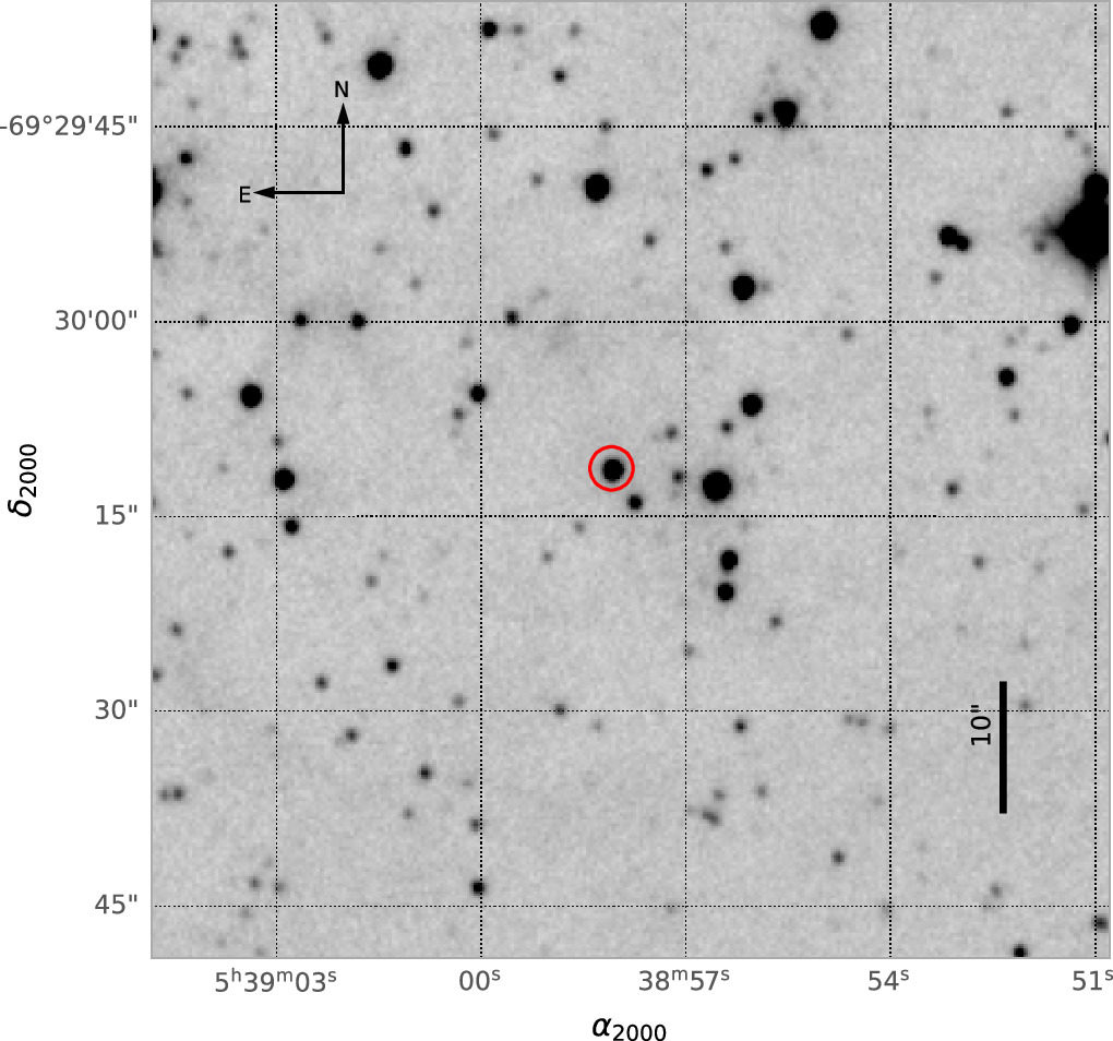
Figure 1. A part of a SOFI Ks -band frame showing a neighborhood of the BLMC-03 system, which is marked with a red circle.
Download figure:
Standard image High-resolution imageUnfortunately, because of randomly appearing patterns in one quadrant of the camera, some of our measurements had to be discarded. However, joining the SOFI data with the VMC Ks photometry, both eclipses are covered, and the flat parts of the light curves (out of the eclipses) are well-defined. As far as we know, our final light curve with 26 data points is the best-covered Ks -band light curve for an extragalactic eclipsing binary system.
2.2. Spectroscopy
We acquired high-resolution optical echelle spectra of BLMC-03 using the UVES spectrograph (Dekker et al. 2000) mounted on the Very Large Telescope (VLT) at Paranal Observatory and the MIKE spectrograph (Bernstein et al. 2003) on the Magellan Clay Telescope at the Las Campanas Observatory (LCO), both in Chile. The setup of the instruments and the reduction procedure are the same as described in Paper I. A total of 17 high-resolution spectra (nine UVES + eight MIKE) were obtained with a typical signal-to-noise ratio near 4000 Å of about 50–60 for UVES and 30–40 for MIKE.
To increase the time coverage of observations, we used in addition seven archival spectra collected with the Magellan Echellette (MagE) spectrograph, also mounted on the Clay telescope at the LCO. These data were used previously by Massey et al. (2012), where a detailed description of the instrument setup, reduction, and calibration can be found. Thus, in total 24 spectra were used for the determination of RVs in a homogeneous way and in the main analysis of the binary system.
We note that Massey et al. (2012) provide four more velocity determinations from the analysis of their spectra acquired with the Inamori–Magellan Areal Camera and Spectrograph (IMACS) instrument on the Baade Telescope at the LCO. We took these data into account in the analysis of the outer (A+B) orbit but did not use them to obtain the final results (see Section 3.1.1 for details).
3. Analysis
The analysis of BLMC-03 is similar to the analyses performed in our previous papers (Papers I and II), with the difference that it takes into account the presence of other bodies (see Sections 3.1.1 and 3.3 below). Similarly to the study of BLMC-02 described in Paper II, we also used NLTE spectral analysis to obtain the temperatures of the components and an independent estimate of their luminosity ratio.
Following the typical process for eclipsing binaries, we model the light and RV curves to characterize the system and obtain the physical parameters of its components. Before performing the main analysis described in detail below, preliminary fits to the available data were done to obtain an approximate characterization of the system and the stars and identify possible complications. The main analysis consists of the determination of RVs of the primary and secondary components (free of higher-level orbital motion) and simultaneous modeling of the light and RV curves corrected for the light travel time effect (LTTE). This is followed by the NLTE spectral analysis. Finally, from the combined results, the physical parameters of the components are derived.
3.1. RVs and Orbital Solution
We started our analysis by determining the RVs of the primary and secondary components of BLMC-03. For that, we applied the broadening function (BF) technique (Rucinski 1992, 1999) to the reduced one-dimensional spectra using the RaveSpan code (Pilecki et al. 2017). As a template spectrum, we used a spectrum of a standard star from the ESO Data Archive that was selected to match the spectral type of the components.
Once we had extracted the RVs from the spectra, we modeled the RV curve taking into account the orbital elements of a spectroscopic binary: period (PA), the orbital semi-amplitudes (KA), the velocity of the center of mass (VA), the reference time (T0,A), the orbital eccentricity (eA), and the argument of periastron passage of the primary component (ωA). We fitted a model to the observed RV curve of each component of the system and obtained a preliminary orbital solution.
3.1.1. Third Body
In the preliminary RV curve analysis, we detected correlated cyclic changes (with a period of about 200 days) in the residual RVs for the primary and secondary components. This was a clear indication of the inner (Aa+Ab) system orbiting the common center of mass (COM) of the higher-order system. As from the light curve analysis, we also obtained significant values for the third light 8 in all considered bands, we concluded that the system is at least a triple, and included the presence of a third body in the RV analysis. In the final model of the Aa+Ab binary, we thus included additional parameters that describe the orbital motion of this binary around the A+B system COM. We then fitted this model to the measured velocities of the primary and secondary components.
Table 1. General Information About the System
| Parameter | Unit | Value |
|---|---|---|
| Our ID | ⋯ | BLMC-03 |
| OGLE ID | ⋯ | LMC-ECL-21568 |
| α2000 | [hh:mm:ss.ss] | 05:38:58.08 |
| δ2000 | [±dd:mm:ss.s] | −69:30:11.3 |
| Orbital period | [days] | 3.225450 |
| I C band | [mag] | 14.212 |
| V band | [mag] | 14.125 |
| V − IC | [mag] | −0.087 |
| Spectral type | ⋯ | O9V+O9.5V a |
Note.
a Massey et al. (2012).Download table as: ASCIITypeset image
To increase the number of data points, we considered adding to our analysis, the RVs measured by Massey et al. (2012) from their IMACS spectra mentioned in Section 2.2. These RVs were measured using a low number of spectral lines: 1, 3, 4, or 6, depending on the spectrum (see Table 6 of Massey et al. 2012). We considered the measurement using just one line as not reliable, and indeed, a quick check showed the difference between the primary and secondary velocities to be about 50 km s−1 too low. The uncertainties for them are also not provided. We thus used in the analysis only measurements based on at least three lines, with determined uncertainties. After doing the fit, we noted, however, that these RVs from the literature, although being marginally consistent within error bars, are all lower than the best model by about 15–20 km s−1. Moreover, this shift is also seen when comparing one of these points with our two measurements done for spectra taken 5 days later. As the data we used for our RV measurements dominate in number and quality, the exclusion of these external measurements leads to practically the same results regarding the A+B system (amplitude change of 0.3σ), and more importantly, negligible changes in the parameters of the inner one (below 0.2σ). Taking all of this into account and to maintain the homogeneity of the measurements, we decided to use, here and in the rest of the analysis, only RV measurements determined by us (uniformly using the BF method) from the UVES, MIKE, and MagE spectra. The final orbital solution for the outer system is shown in Figure 2, and the properties of its orbit are given in Table 2.
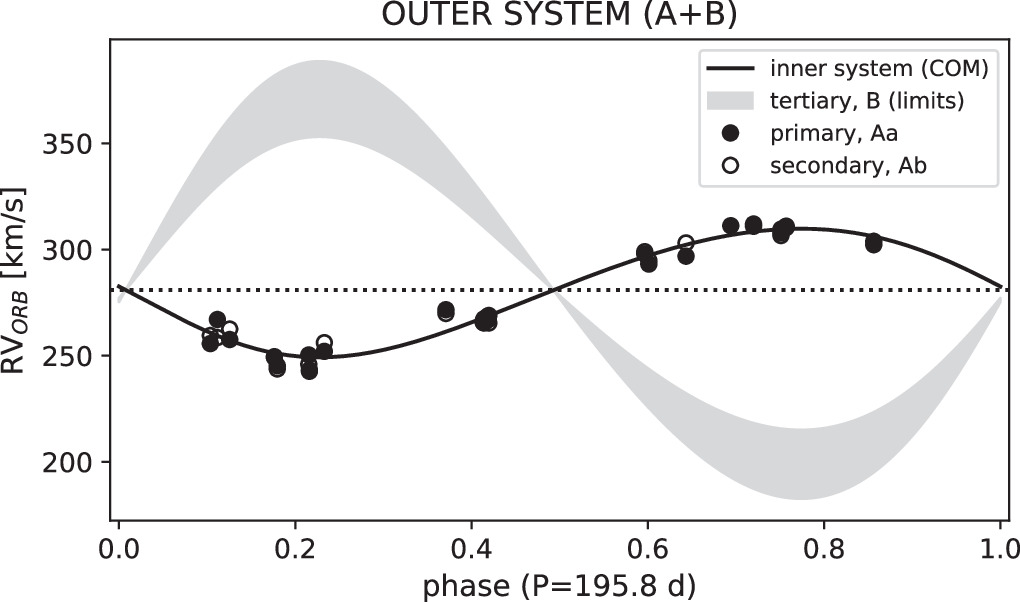
Figure 2. RV of the inner (Aa-Ab) system center of mass and the range of possible velocities of the tertiary component (assuming it is single for the superior limit). Velocities of the primary and secondary components are residuals after the subtraction of RVs from the inner binary model.
Download figure:
Standard image High-resolution imageTable 2. Orbital Elements of the Outer A+B Orbit of BLMC-03
| Parameter | Unit | Value |
|---|---|---|
| PB | [days] | 195.78 ± 0.13 |
| T0,B | [days] | 8038.3 ± 1.0 |
| eB | ⋯ | 0.086 ± 0.024 |
| ωB | [deg] | 123 ± 15 |
| KA | [km s−1] | 30 ± 0.6 |

| [km s−1] | 69 a |

| [km s−1] | 103 |
Note.
a Assuming the third object is a single star.Download table as: ASCIITypeset image
The inclusion of the third body in the orbital solution has decreased the scatter (rms) of residuals from about 22–4 km s−1. The orbital period of the outer system converged firmly at PA+B = 195.78 ± 0.13 days, resulting in the period ratio between the outer and inner systems of PA+B/PA ≈ 61. A mass estimate for the tertiary will be derived later, once we have the final masses of the inner components. The main result from this part of the analysis is RVs of the primary and secondary components free of additional orbital movement around the outer A+B system COM and a preliminary orbital solution, which will be used as an input in the final modeling.
3.1.2. Stellar Rotation
From the BF method, the projected rotation velocities of the components of the system ( ) were also obtained. The broadening function response for one of the spectra is presented in Figure 3. We have determined
  for various spectra taken close to the orbital quadratures, where the profiles are well separated, taking an average. To obtain the true rotation velocities, we assume the inclination of the rotation axes to be the same as the orbital inclination and correct measured velocities for the rotation velocity of the template star. We did not correct for instrumental broadening because it is negligible compared with the measured velocities. The rotation velocities, obtained as described, are about 70 and 80 km s−1 for the primary and secondary components, respectively.
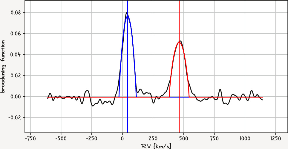
Figure 3. An example of a BF profile for one of the analyzed spectra. Apart from RVs, rotational velocities are measured, which are lower than typical for early-type stars.
Download figure:
Standard image High-resolution imageThe final values are later used in the modeling in the Phoebe code (Prša & Zwitter 2005) as a synchronization parameter (F), defined as the ratio between the rotational and orbital angular velocity. This information is important for the modeling, as rotation changes the shape of stars, which influences the light (mostly) and RV (to a lower extent) curves. For both components, the measured rotational velocities are subsynchronous (F1 = 0.61, F2 = 0.75). This means that either their rotation is slower than the angular orbital motion, or their rotation axes have inclinations lower than the orbital one. Note that we do not compare our rotation velocities with a pseudo-synchronous velocity (defined by the orbital angular velocity at periastron) as the difference between the synchronous and pseudo-synchronous velocity for the very low eccentricity of BLMC-03 is insignificant.
3.2. Light and RV Curve Modeling
The rest of the analysis closely resembles the one for BLMC-02 described in Papers I and II, where a detailed description is provided. In short, we have used a Python wrapper to the Phoebe 1 code to obtain a simultaneous solution to the observed light and RV curves. For that, we used a Markov Chain Monte Carlo analysis, which also provides reliable uncertainties and lets us find correlations between fitted parameters. The initial parameter values were taken from the aforementioned preliminary low-resolution analysis. A slight difference from the standard analysis was the usage of RVs of the components corrected for the orbital motion around the outer system's center of mass (in comparison to using the velocities directly).
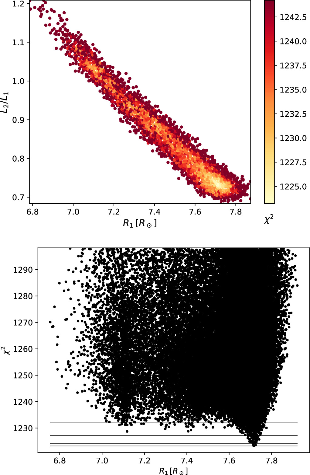
As typical for well-detached, non-totally eclipsing systems, we found a slight degeneracy between the parameters of the component stars. This can be seen, for example, in the correlation between the radius of the primary component (R1) and the luminosity ratio (L2/L1) in Figure 4 (top). The solution is well-defined (with small, symmetric uncertainties) within 1σ but strongly asymmetric for 3σ uncertainties, as can be seen in the χ2 plot for R1 in the bottom panel of Figure 4. However, we note that along the L2/L1–R1 relationship (top panel) the flux ratio F2/F1 =  remains constant. We measure F2/F1 = 0.971 ± 0.002 in the V band and 0.968 ± 0.004 in both the IC
and Ks
bands. This flux ratio will be used to constrain the effective temperature difference between the primary and secondary components in the non-LTE spectral analysis described in Section 3.4, which in turn will be used to obtain the final, nondegenerate solution.
remains constant. We measure F2/F1 = 0.971 ± 0.002 in the V band and 0.968 ± 0.004 in both the IC
and Ks
bands. This flux ratio will be used to constrain the effective temperature difference between the primary and secondary components in the non-LTE spectral analysis described in Section 3.4, which in turn will be used to obtain the final, nondegenerate solution.

Figure 4. Top: results from the Markov Chain Monte Carlo analysis showing a correlation between the radius of the primary star and the luminosity ratio. Bottom: the χ2 values vs. the radius of the primary star for the models calculated in the analysis.
Download figure:
Standard image High-resolution image3.3. O − C Analysis
Looking at the light curve models obtained in the previous section, we found a significant residual scatter around eclipses (see Figure 5). To determine the cause of this scatter and try to independently check the orbital parameters of the third body (B), we performed an O − C analysis similar to that described in Pilecki et al. (2021), using the long-time-span light curves from the EROS-2 and OGLE projects. The strongest variation seen in the O − C diagram (see Figure 6) indeed looked like it was caused by the orbital motion, but to our surprise, its period was determined as 2550 ± 30 days. The shorter-period variability previously detected in RVs was also found with a period of 195.3 ± 0.5 days but with much lower amplitude, consistent with the spectroscopic orbit determined in Section 3.1.1 (KA,O − C = 26 ± 3 compared to KA,RV = 30.0 ± 0.6). This variability is best seen in the data set of OGLE-IV (HJD >2455000 days), which has the highest density and quality of measurements. Both variabilities can be described by the LTTE, as shown by the red line fit in Figure 6. Apart from that, no other secular, cyclic, or erratic changes were detected.
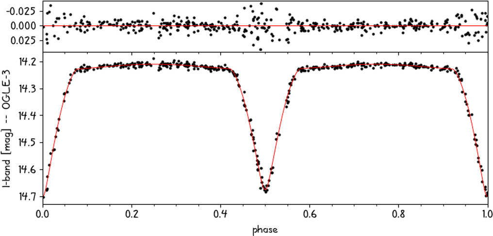
Figure 5. IC -band light curve for BLMC-03 without accounting for the presence of the fourth component. The best model fit is shown as a red line. A high residual scatter can be seen around eclipses.
Download figure:
Standard image High-resolution image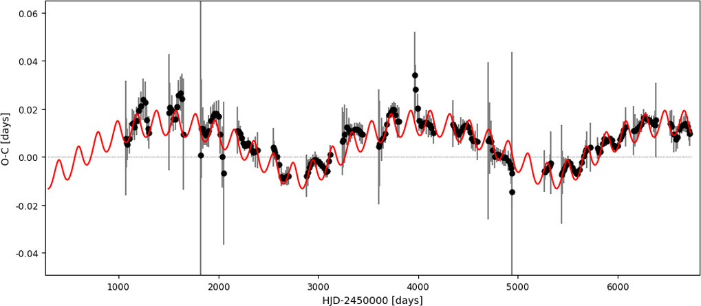
Figure 6. O − C diagram showing the phase shifts between the data from around the given date and the average model. The influence of two extra components can be seen. The red line is the fit to the LTTE induced by the third and fourth body.
Download figure:
Standard image High-resolution imageWith these results, we could not only confirm the existence and the orbital period of the third component found in the analysis of RVs but also the presence of a fourth component. The system is thus at least a quadruple with the configuration (Aa+Ab)+B+C. Because of a wider orbit, the influence of the fourth body (C) on the phase shift of the eclipsing variability of the A system is much stronger than that of the third body (B). To account for this periodic phase shift we subtracted it from the light and RV curves by adjusting the measurement time by the value obtained from the LTTE fit. We then modeled these corrected data and obtained new model fits. As can be seen in Figure 7, the extra scatter in the eclipses disappeared almost completely. As the depths and shape of the eclipses are now better defined, some parameters, such as the radius, temperature ratio, and the third light parameter, changed slightly. The final fitted values are close to the ones determined before (within uncertainties) but are more precise. The degeneracy also decreased. The final RV curve is shown in Figure 8.
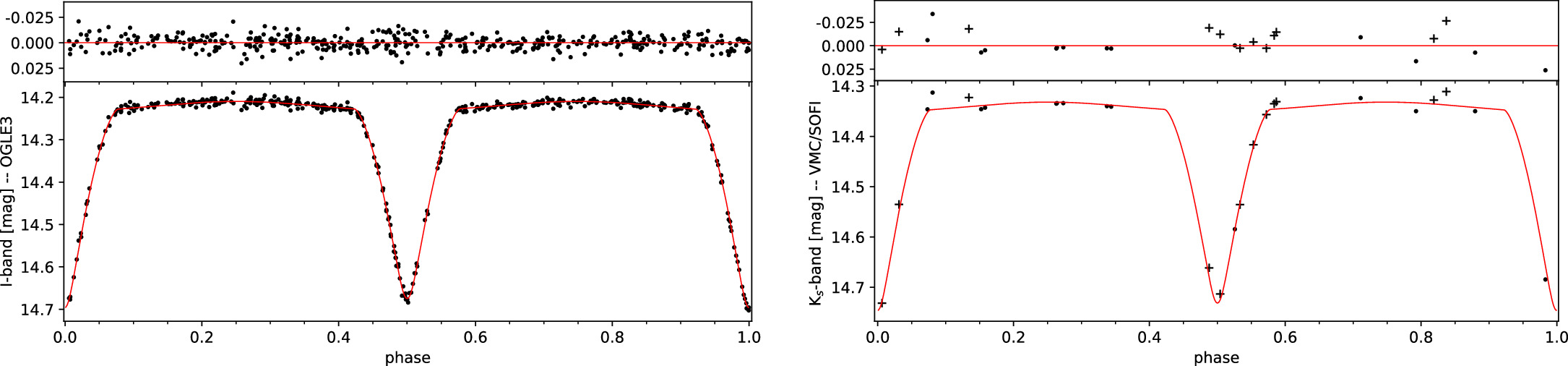
Figure 7. IC - and Ks -band light curves for BLMC-03 corrected for the gravitational influence of the fourth component. The residual scatter around eclipses disappeared almost completely. In the right panel, VMC and SOFI data are represented by points and crosses, respectively.
Download figure:
Standard image High-resolution image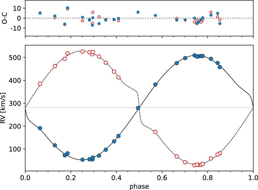
Figure 8. Orbital solution for the inner binary system. Measured RVs for the primary (blue) and secondary (red) components are shown with residuals in the upper panel.
Download figure:
Standard image High-resolution image3.4. Spectral Analysis and Reddening Determination
The purpose of the non-LTE spectral analysis of the observed binary is primarily to determine the effective temperatures of the components and interstellar reddening and extinction. This enables us to discuss the physical nature and evolutionary status of the components and to constrain interstellar reddening and extinction, providing intrinsic colors and surface brightnesses as well as an independent estimate of the distance. We also used this analysis to independently find the best solution along the slight degeneracy described in Section 3.2.
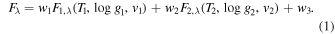
We proceed in a very similar way as in Paper II. We use the non-LTE model atmosphere code FASTWIND (Puls et al. 2005; Rivero González 2012) and calculate normalized flux spectra F1,λ and F2,λ for the primary and secondary stars, respectively, and then combine those to a composite spectrum through
Ti
,  , and vi
denote effective temperature, gravity, and RV of the primary and secondary components. The weight w3 accounts for the contribution of the additional light (the third light parameter in the binary model) described in the previous sections and is defined as
, and vi
denote effective temperature, gravity, and RV of the primary and secondary components. The weight w3 accounts for the contribution of the additional light (the third light parameter in the binary model) described in the previous sections and is defined as

where L1 and L2 are the V-band luminosities of the primary and secondary components, and L3 is the total luminosity of all additional components. From the photometry fits discussed above, we obtain w3 = 0.19 ± 0.01. The weights w1 and w2 represent the continuum contributions by the primary and secondary components, respectively, and are given by

and

We use the observed flux ratio given in Section 3.2 to calculate w1 and w2, together with the primary and secondary radii and stellar gravities along the solutions seen in Figure 4 as obtained from the light-curve and RV-curve modeling described in previous sections.
In the first step, we determine the effective temperature difference of ΔT = T1 − T2 between the primary and secondary components. We use FASTWIND model spectral energy distributions (SEDs) to calculate stellar V-band fluxes and compare their ratio with the observed value. For the gravities from the binary model (as mentioned above) and with temperatures between 30,000 and 39,000 K, the observed ratio leads to ΔT = 500 ± 100 K. We then calculate a grid of composite spectra close to binary quadrature with this temperature difference ΔT varying the primary temperature between 31,000 and 39,000 K for each pair of radii and gravities. As in Paper II, we adopt four values of the helium abundance N(He)/N(H), 0.08, 0.09, 0.1, and 0.15, two values for the microturbulence vturb = 10 and 15 km s−1, and metallicity of [Z] = log Z/Z⊙ = −0.35 (Urbaneja et al. 2017). We calculate normalized spectra with line profiles accounting for the observed rotational velocities and the spectral resolution of the spectrographs by convolving with the corresponding broadening profiles.
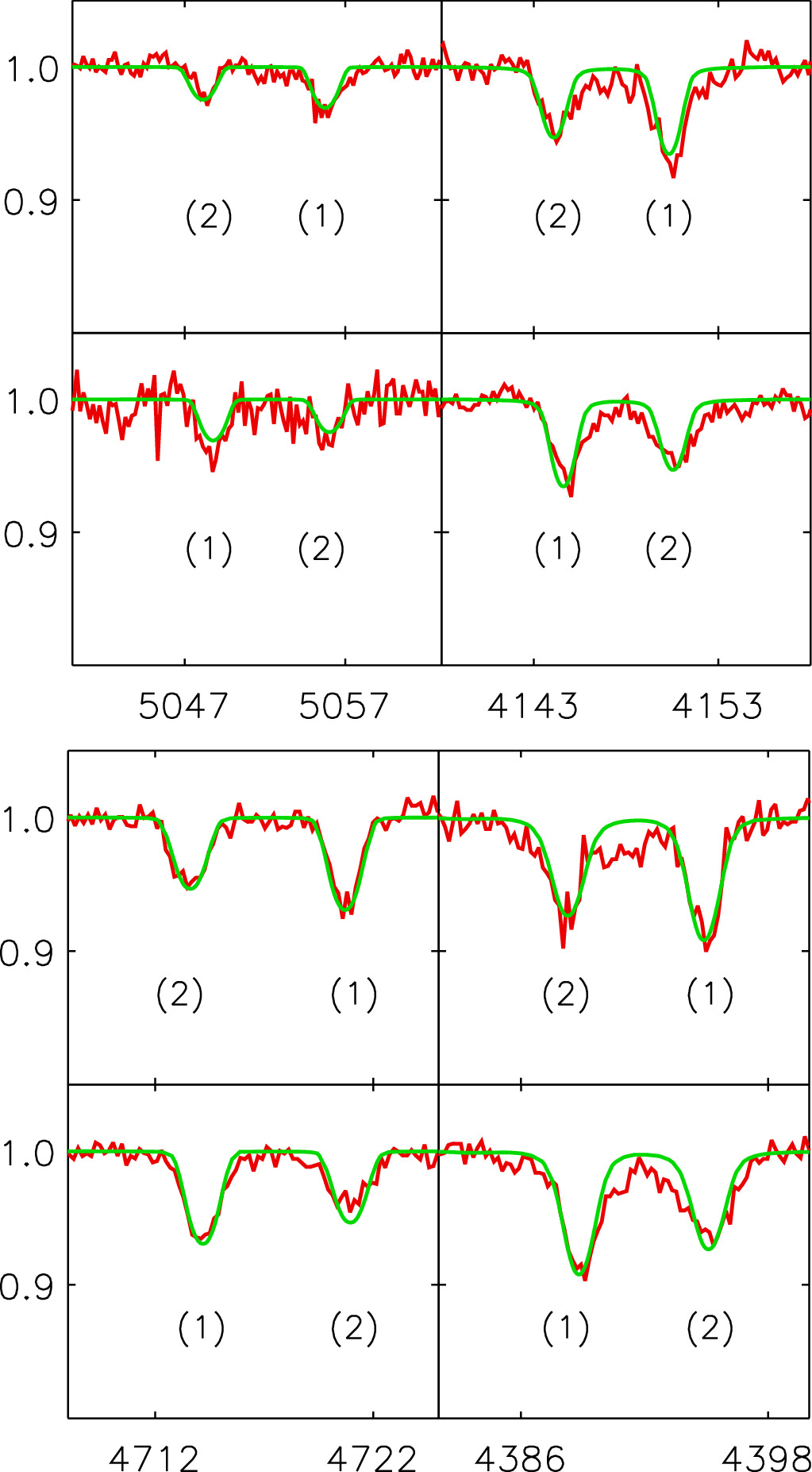
In our analysis, we proceed exactly as in Paper II. We select the same set of He i and He ii lines and compare the model and observed spectra by calculating the χ2 values for all radii, temperatures, helium abundances, and microturbulence values and use the minimum of χ2 combined with Monte Carlo simulations to constrain the stellar parameters of the system. We obtain 34,250 ± 500 and 33,750 ± 500 K for the effective temperatures of the primary and secondary components, respectively, together with a helium abundance of N(He)/N(H) = 0.09±0.01 and a microturbulence of vturb = 10 km s−1. Our best solution is obtained for the primary radius of R1 = 7.7 R⊙, which confirms the best solution from the binary modeling. Examples of the fits of the helium lines with the final model are shown in Figures 9 and 10.

Figure 9. Fit of He i lines with the best composite binary model spectrum obtained from the χ2 analysis. The upper figure shows He i 5048 (left) and He i 4143 (right), and the lower figure He i 4713 (left) and He i 4387 (right). The upper row in each figure corresponds to the superposition of three UVES spectra around phase 0.75 and the lower row to three MIKE spectra at phase 0.2. The line contributions from the primary and secondary stars are indicated by (1) and (2), respectively.
Download figure:
Standard image High-resolution image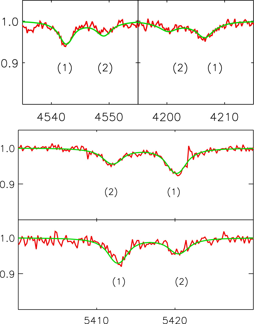
Figure 10. Fit of He ii lines. The upper figure shows the MIKE spectrum of He ii 4541 (left) and the UVES spectrum of He ii 4200. The lower spectrum displays the fits of the UVES (upper row) and MIKE (lower row) spectra of He ii 5411.
Download figure:
Standard image High-resolution image3.4.1. Reddening and Extinction
In the next step, we determine the interstellar reddening and extinction. This is crucial for an independent estimate of distance and a measurement of intrinsic stellar surface brightness and colors. For this purpose, we use multiband photometry outside the eclipses, corrected for the contribution of the additional components. In the Johnson–Cousins system, from the literature, we have the apparent magnitude of B =14.17 ± 0.05 mag (Testor & Niemela 1998; Massey et al. 2002; Zaritsky et al. 2004), as well as V = 14.34 ± 0.03 mag and IC = 14.46 ± 0.03 mag from our light-curve modeling (the system brightness at phase 0.15). The applied corrections for the additional light were 0.18, 0.20, and 0.24 mag, respectively. Using our binary model, we also derived consistently out-of-eclipse Gaia magnitudes from available light curves (DR3, Gaia Collaboration 2023) with GB = 14.22 ± 0.03 and GR = 14.38 ± 0.030 mag, where the third light corrections of 0.20 and 0.23 mag were applied. From our modeling, we also derived the near-IR magnitudes of BLMC-03 in J (VMC data) and the Ks band (VMC+SOFI). We adopt J = 14.61 ± 0.04 mag and Ks = 14.70 ± 0.05 mag with the third light corrections of 0.28 and 0.36 mag, respectively.
We then proceed exactly in the same way as in Paper II and use the composite SED of our final model of the primary and secondary stars to calculate reddened model colors (B − V), (GB − V), (V − GR ), (V − IC ), (V − J), and (V − Ks ) in the same passbands as observed assuming a grid of E(B − V) and RV = AV /E(B − V) values in the ranges from 0.0–0.3 and 1.0–7.0 mag, respectively. From the χ2 comparison between calculated and observed colors, we determine the best pair of E(B − V) and RV at the minimum of χ2. In a Monte Carlo simulation, we modify the observed colors assuming a Gaussian distribution of uncertainties and construct probability distribution functions N(E(B − V)), N(RV ), N(AV ), and N(m − M) for reddening, the ratio of extinction to reddening, extinction, and distance modulus, respectively. Figure 11 shows the result assuming the monochromatic reddening law by Maíz Apellániz et al. (2014) and Maíz Apellániz et al. (2017). We have also applied the reddening laws by Cardelli et al. (1989), O'Donnell (1994), and Fitzpatrick (1999), which yield very similar results. We obtain as average values E(B − V) = 0.16 ± 0.02 mag, RV = 3.2 ± 0.8, AV = 0.51 ± 0.08 mag, and a distance modulus of m − M = 18.59 ± 0.06 mag.
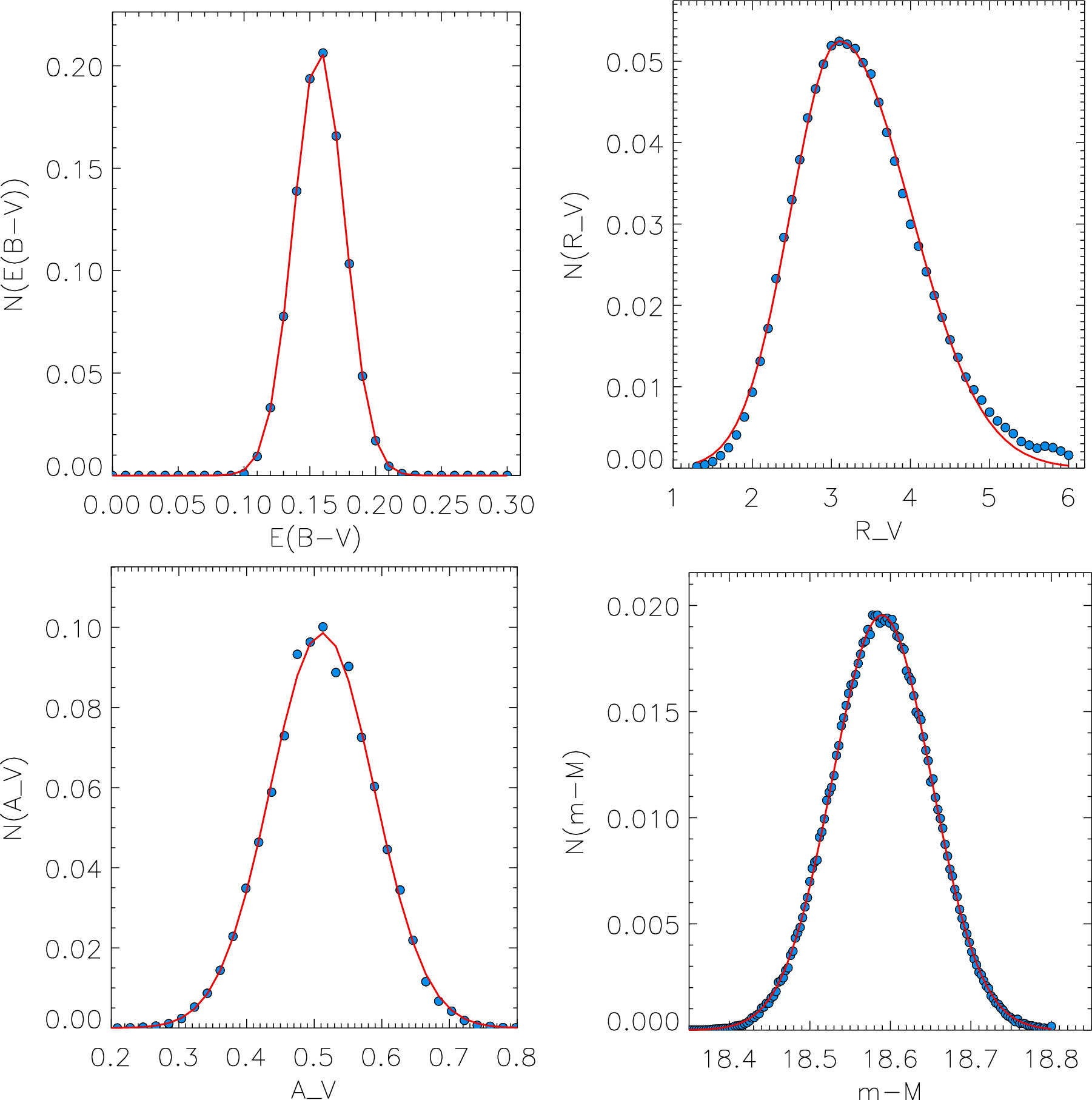
Figure 11. Probability distributions (blue circles) and Gaussian fits (red) obtained from the Monte Carlo fit of observed colors as described in the text. The red curves represent Gaussian fits. Top left: N(E(B − V)), top right: N(RV ), bottom left: N(AV ), bottom right: N(m − M).
Download figure:
Standard image High-resolution image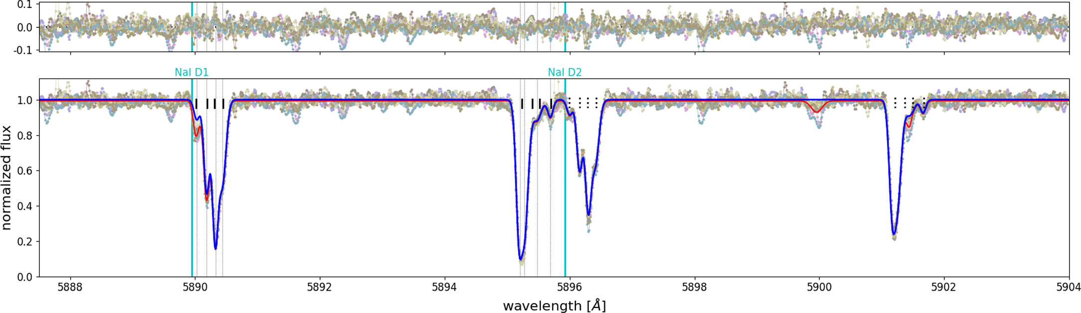
Figure 12. A multicomponent fit to the sodium doublet at 5890 Å. Individual components are marked with thick black vertical lines. For both the LMC and Milky Way, four components were identified. The red line shows the fit to the data, including extra lines, while the blue one marks the profiles of the sodium lines only. Multiple spectra (lines of different colors) are fitted at once. The resulting reddening E(B − V) is 0.145.
Download figure:
Standard image High-resolution image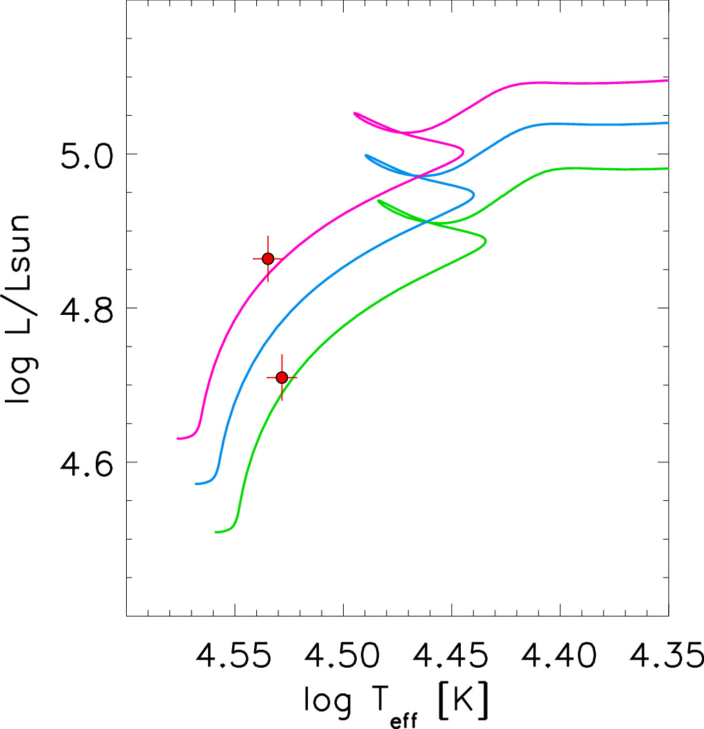
Figure 13. Location of the binary components in the HRD compared to MESA evolutionary tracks with ZAMS masses of 18 (green), 19 (blue), and 20 (pink) M⊙.
Download figure:
Standard image High-resolution image3.4.2. Reddening from the Sodium Line
Similar to the systems analyzed in previous papers, we performed an independent determination of the reddening value through the measurement of the equivalent widths of the sodium doublet lines. The fit is shown in Figure 12. From the calibration of Munari & Zwitter (1997), we then determined the reddening values for the Milky Way and LMC components separately. For the Milky Way, E(B − V) = 0.070, while for the LMC E(B – V) = 0.075. The total reddening is E(B − V) = 0.145, in good agreement with the value obtained from the spectral analysis.
4. Results
To obtain the final solution, we combined the results from the Monte Carlo analysis of the light and RV curves corrected for the presence of extra components with those from the NLTE spectroscopic analysis. The final results are summarized in Table 3, where we list the physical parameters of the components together with the orbital properties of the inner system. Note that the difference in temperature between the primary and secondary components is determined much better than their individual temperatures. From the binary model ΔT = 510 ± 40, which is almost identical to the one obtained from the spectroscopic analysis (ΔT = 500 ± 100).
Table 3. Physical Parameters and Other Properties of the Inner Binary (A)
| Parameter [Unit] | Primary (Aa) | Secondary (Ab) |
|---|---|---|
| Mass [M⊙] | 19.02 ± 0.12 | 17.50 ± 0.13 |
| Radius [R⊙] | 7.70 ± 0.05 | 6.64 ± 0.06 |
 [cgs] [cgs] | 3.944 ± 0.005 | 4.035 ± 0.007 |
| Temperature [K] | 34,250 ± 500 | 33,750 ± 500 |
 [K] [K] | 500 ± 100 | |

| 0.9851 ± 0.0011 | |
 [L⊙] [L⊙] | 4.854 ± 0.010 | 4.700 ± 0.003 |
| j21,V = F2/F1(V) | 0.971 ± 0.002 | |
| V [mag] | 14.963 ± 0.021 | 15.285 ± 0.025 |
| IC [mag] | 15.086 ± 0.021 | 15.413 ± 0.024 |
| Ks [mag] | 15.316 ± 0.029 | 15.644 ± 0.029 |
| vrot [km s−1] | 70 ± 7 | 80 ± 8 |
| E(B − V) [mag] | 0.16 ± 0.02 | |
| Orbital period, P [days] | 3.2254367 ± 0.0000003 | |
| Semimajor axis [R⊙] | 30.48 ± 0.07 | |
| Orbital inclination, i | 87.43 ± 0.21 | |
| Eccentricity, e | 0.0006 ± 0.0003 | |
| Argument of periastron, ω [rad] | 0.3 ± 1.0 | |
Apsidal motion,  [rad/d] [rad/d] | -0.005 ± 0.004 | |
| Orbital semiamplitude, K [km s−1] | 228.5 ± 1.3 | 248.7 ± 1.1 |
| Systemic velocity, γ [km s−1] | 280.7 ± 0.4 | |
| Mass ratio, q = m2/m1 | 0.919 ± 0.007 | |
Note. Passband magnitudes are observed (reddened) values. For ω, any value is possible within 3σ.
Download table as: ASCIITypeset image
The distance modulus of m − M = 18.59 ± 0.06 mag obtained through our spectral analysis and de-reddening can be compared with the value of 18.45 ± 0.02 mag derived from the 1% precision distance to the LMC determined by Pietrzyński et al. (2019) and a small geometrical correction accounting for the location of the system within the LMC using the geometrical LMC model by van der Marel & Kallivayalil (2014). Being 2σ larger, it agrees just within the error margins. It is interesting to note that for BLMC-02 analyzed in Paper II, we also found a spectroscopic distance modulus of 0.05 mag larger. This may hint at a small systematic effect caused by the use of our non-LTE model atmospheres, but we will need the analysis of additional objects to investigate this further.
With our determination of effective temperatures and luminosities, we can discuss the evolutionary status of the O-star binary system in the Hertzsprung–Russell diagram (HRD). In Figure 13, we show MESA evolutionary tracks (Choi et al. 2016; Dotter 2016) for 18–20 M⊙ and the location of the primary and secondary stars in the HRD. From the MESA grid of evolutionary models, we have selected tracks with a metallicity of [Z] = −0.5 and without rotation. We have selected the latter because the rotational velocities are relatively small compared to the alternative in the MESA grid with vrot/vcrit = 0.4. According to the tracks, the binary components have a consistent age of 6.3 Myr. The tracks indicate masses of 20 and 18 M⊙, slightly higher than obtained with our analysis but at the margin of the uncertainties.
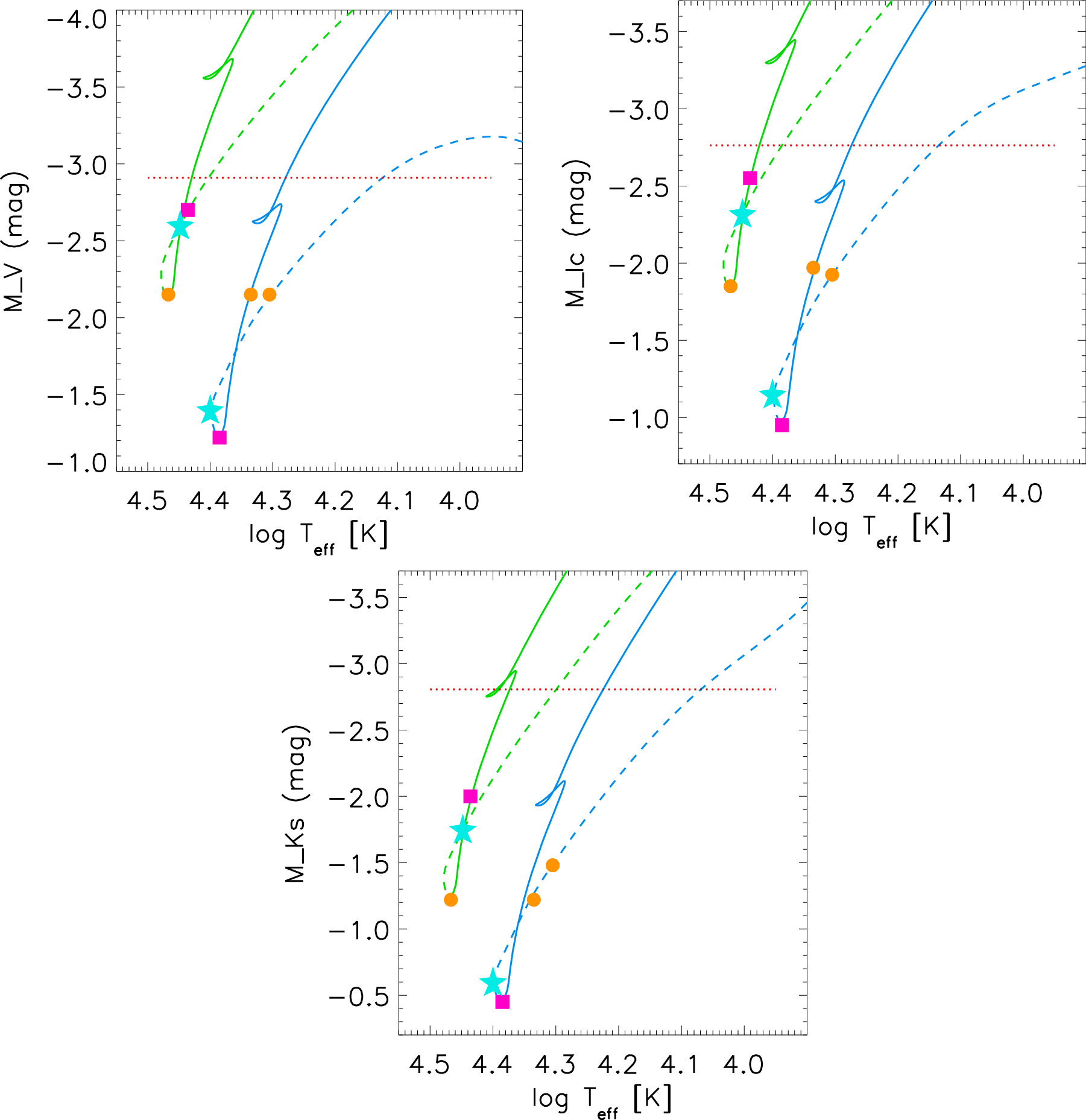
Having determined the masses of the inner system components, we can also estimate them for the additional components. Assuming an orbital inclination of 90° (outer orbit seen edge-on) from the spectroscopic orbit of the A system, the minimum mass of the tertiary is estimated to be about MB ∼ 10.7 M⊙. With this limit at hand, and having the orbital semiamplitude of the A+B system derived from the detected LTTE (KAB = 8.6 ± 0.4), we obtain the minimum mass of the fourth component of MC ∼ 7.3 M⊙. Moreover, as we know that these objects provide about 20% of the total system light and are not visible in the spectra, the individual components should be less massive than the primary and secondary components individually. This puts a conservative upper limit to the mass of about 17.5 M⊙ (the mass of the secondary component) for a single star. From the fact that the more inclined the outer orbit is, the more massive tertiary we would obtain, we can also constrain the inclination of the A+B system, iA+B ≳ 42°, assuming B is a single star. With the same assumption, we expect MB to be close to the lower limit and to have an inclination similar to that of the inner system, although the orbits do not necessarily have to be coplanar.
We can use the additional light found in our light curve analysis in Section 3.2 for an attempt to further constrain the nature of the third and fourth objects. With the magnitude corrections given above, we obtain V = 16.05 ± 0.03 mag, V − IC = 0.06 ± 0.02 mag, and V − Ks = 0.35±0.04 mag. With E(B − V) = 0.16 mag and RV = 3.2 (see the previous section), we can correct for extinction and calculate intrinsic colors and magnitude: V0 = 15.54 ± 0.08 mag, (V − IC )0 = −0.15 ± 0.10 mag and (V − Ks )0 = −0.10±0.10 mag.
With a distance modulus of 18.45 (see above), we then obtain absolute magnitudes MV
= −2.91 ± 0.08 mag,  = −2.76 ± 0.06 mag, and
  = −2.80 ± 0.05 mag. This allows us to compare the joint magnitudes of the objects with MESA evolutionary tracks of 7.4 and 11 M⊙, corresponding to the minimum masses of the fourth and third objects, respectively. This is done in Figure 14, where we show absolute magnitudes in V, IC
, and Ks
versus effective temperature. The MESA tracks are from the same evolutionary grid as used in Figure 13. They include pre-main-sequence evolution toward the zero-age main sequence (ZAMS) and post-main-sequence evolution away from ZAMS. The observed absolute magnitudes of the combined third and fourth objects are also shown in each panel.
= −2.80 ± 0.05 mag. This allows us to compare the joint magnitudes of the objects with MESA evolutionary tracks of 7.4 and 11 M⊙, corresponding to the minimum masses of the fourth and third objects, respectively. This is done in Figure 14, where we show absolute magnitudes in V, IC
, and Ks
versus effective temperature. The MESA tracks are from the same evolutionary grid as used in Figure 13. They include pre-main-sequence evolution toward the zero-age main sequence (ZAMS) and post-main-sequence evolution away from ZAMS. The observed absolute magnitudes of the combined third and fourth objects are also shown in each panel.
Figure 14. Evolutionary constraints on the third and fourth objects. We show MESA evolutionary tracks with ZAMS masses of 7.4 (blue) and 11 (green) M⊙, corresponding to the minimum masses of the fourth and third objects, respectively. Absolute magnitudes in the V band (upper left), IC (upper right), and the Ks band (lower panel) are plotted vs. effective temperature. The dashed part of the tracks corresponds to the evolution toward the ZAMS. The horizontal red-dotted line corresponds to the de-reddened total absolute magnitude of the combined third and fourth objects. The orange circles, pink squares, and cyan stars on the tracks are defined and discussed in the text.
Download figure:
Standard image High-resolution image
Figure 14 indicates that only a small range of effective temperature of the tracks is compatible with the observed magnitudes. From the V band, we see immediately that the effective temperature of the third object (represented by the track with 11 M⊙) is tightly constrained to an evolutionary phase very close to the ZAMS with log Teff ≥ 4.4. This also restricts the evolutionary status of the fourth object (the track with 7.4 M⊙) because the combined brightness of both objects needs to match the observed magnitude shown as the red-dotted line. At the minimum brightness of the third object, the fourth object must have a very similar magnitude, as indicated by the orange circles on the tracks. The maximum possible brightness of the third object is constrained through the minimum V-band magnitude of the fourth object on the 7.4 M⊙ track. The pink squares on each track define the corresponding evolutionary phases and magnitudes. The range between the pink squares and the orange circles on both tracks describes the evolutionary phase during which the joint brightness of both objects matches the V-band observation. The cyan stars provide an example within this range.
We then use exactly the same evolutionary phases represented by the orange circles, pink squares, and cyan stars in the plot of  in Figure 14. Combining the corresponding magnitudes on the two tracks, we find that they also agree with the observation within the error margins. However, we encounter a severe discrepancy with the observations for
  , as shown in Figure 14. The combined magnitudes of the orange circles, cyan stars, and pink squares, respectively, are 0.6–0.75 mag too faint. This may indicate an IR excess of these objects, for instance, caused by a circumstellar disk or an even more complex structure of the system with a possible multiplicity of the B and C components.
In a similar analysis, we also found that the evolutionary track for a star of 16 M⊙ would lie entirely above the red-dotted line in the V-band panel of Figure 14 (passing slightly below it for the I band), i.e., the star at any evolutionary stage would be brighter than the additional light we found. This puts a stronger (than the mass of the secondary) mass limit of 16 M⊙ on the third and fourth components (or individual stars they consist of in the case any of them is a binary itself).
5. Conclusions
From our multi-method analysis, the BLMC-03 system resulted in being much more complex than expected. We found strong evidence for the existence of two extra components orbiting around the studied binary system. Each of these two extra components may be a binary itself, but we have no direct evidence for that, apart from a small hint from the additional light in the Ks band, which may suggest more than two but cooler and redder stars in the system.
This (at least) quadruple system belongs to the less common group of 2 + 1 + 1 systems (2 + 2 are more frequent; see, e.g., Tokovinin 2014). The period ratios are PA+B/PA = 60.7 and PAB+C/PA+B = 13. The system is thus relatively tight for a three-tier hierarchical system.
One may question if such a complex system can be used for our final goal of the calibration of the SB-C relation. However, we have full control over the additional light in the system and take into account the effects of additional components on the measured quantities. As a result, the accuracy and precision of determined parameters are comparable to those for our other systems. One may also argue that it is better to have a binary as a part of a multiple system with detected additional components than a binary with such components not yet detected. This also points to the importance of high-quality data and a detailed study of any extragalactic binary system that will be used in the future for distance measurement.
Acknowledgments
We thank Dr. Nidia Morrell, Dr. Philip Massey, and Dr. Kathryn Neugent for sharing the MagE spectra of BLMC-03 with us. We also thank Nidia Morrell for acquiring a few additional recent MIKE spectra that helped constrain the outer orbit. The research leading to these results has received funding from the European Research Council (ERC) under the European Union's Horizon 2020 research and innovation program under grant agreement No. 951549 (project UniverScale) and from the National Science Center, Poland grant BEETHOVEN UMO-2018/31/G/ST9/03050. R.P.K. has been supported by the Munich Excellence Cluster Origins funded by the Deutsche Forschungsgemeinschaft (DFG; German Research Foundation) under Germany's Excellence Strategy EXC-2094 390783311. M.T., B.P., and G.P. received support from the Munich Institute for Astro-, Particle- and BioPhysics (MIAPbP), which is also funded by the DFG (German Research Foundation) under Germany's Excellence Strategy EXC-2094 390783311. B.P. acknowledges funding from the Polish National Science Center grant SONATA BIS 2020/38/E/ST9/00486. We also acknowledge support from the Polish Ministry of Science and Higher Education under grant No. DIR-WSIB.92.2.2024. This research was based on data collected under the Polish-French Marie Skłodowska-Curie and Pierre Curie Science Prize awarded by the Foundation for Polish Science.
This research is based on observations collected at the LCO and the European Southern Observatory under ESO programs: 098.D-0263(A), 0100.D-0339(A), 0102.D-0469, and 102.D-0590 (B).
This research has made use of NASA's Astrophysics Data System Service.
Facilities: VLT:Kueyen (UVES) - , Magellan:Clay (MIKE and MagE) - Magellan II Landon Clay Telescope.
Software: ESO Reflex9 http://www.eso.org/sci/software/esoreflex/ (Freudling et al. 2013) PHOEBE10 http://phoebe-project.org/1.0 (Prša & Zwitter 2005), RaveSpan11 https://users.camk.edu.pl/pilecki/ravespan/index.php (Pilecki et al. 2017), FASTWIND (Puls et al. 2005; Rivero González 2012).
Footnotes
- *
Based on observations collected at the European Southern Observatory, Chile.
- †
This paper includes data gathered with the 6.5 m Magellan Clay Telescope at Las Campanas Observatory, Chile.
- 7
The exact number depended on the observing conditions.
- 8
The parameter known as a third light in binary modeling describes any additional light that does not come from the components of the eclipsing binary system.