


Abstract
X-ray spectroscopy of heavily obscured active galactic nuclei (AGN) offers a unique opportunity to study the circumnuclear environment of accreting supermassive black holes. However, individual models describing the obscurer have unique parameter spaces that give distinct parameter posterior distributions when fit to the same data. To assess the impact of model-specific parameter dependencies, we present a case study of the nearby heavily obscured low-luminosity AGN NGC 3982, which has a variety of column density estimations reported in the literature. We fit the same broadband XMM-Newton+NuSTAR spectra of the source with five unique obscuration models and generate posterior parameter distributions for each. By using global parameter exploration, we traverse the full prior-defined parameter space to accurately reproduce complex posterior shapes and inter-parameter degeneracies. The unique model posteriors for the line-of-sight column density are broadly consistent, predicting Compton-thick NH > 1.5 × 1024 cm−2 at the 3σ confidence level. The posterior median intrinsic X-ray luminosity in the 2–10 keV band was found to differ substantially, however, with values in the range log L2–10 keV/ erg s−1 = 40.9–42.1 for the individual models. We additionally show that the posterior distributions for each model occupy unique regions of their respective multidimensional parameter spaces and how such differences can propagate into the inferred properties of the central engine. We conclude by showcasing the improvement in parameter inference attainable with the High Energy X-ray Probe, with its uniquely broad, simultaneous, and high-sensitivity bandpass of 0.2–80 keV.
Export citation and abstract BibTeX RIS

Original content from this work may be used under the terms of the Creative Commons Attribution 4.0 licence. Any further distribution of this work must maintain attribution to the author(s) and the title of the work, journal citation and DOI.
1. Introduction
X-ray surveys have revealed that obscured active galactic nuclei (AGNs) with equivalent hydrogen column densities NH > 1022 cm−2 greatly outnumber AGNs with less obscured sightlines, in the local Universe (e.g., Ricci et al. 2017b) as well as at higher redshifts (e.g., Buchner et al. 2014; Ueda et al. 2014; Brandt & Alexander 2015). Although in some cases obscuration could be produced by material in the host galaxy (e.g., Buchner et al. 2017; Gilli et al. 2022; Andonie et al. 2024), the highest Compton-thick column densities (NH > 1.5 × 1024 cm−2) observed at low redshifts are likely dominated by a parsec-scale circumnuclear obscurer surrounding the central accreting supermassive black hole (SMBH), akin to the axisymmetric obscurer invoked in early unified schemes (Antonucci 1993; Urry & Padovani 1995; Netzer 2015; Ramos Almeida & Ricci 2017).
In the X-ray band, the combined effects of photoelectric absorption, fluorescence, and Compton scattering from obscuring material give rise to a characteristic "reflection spectrum" that can dominate over any other AGN signatures if the line-of-sight NH is sufficiently above the Compton-thick limit (i.e., NH ≳5 × 1024 cm−2; Setti & Woltjer 1989; Murphy & Yaqoob 2009; Brightman et al. 2015). The prominent reflection spectrum thus makes X-ray spectroscopy of so-called "reflection-dominated" Compton-thick AGNs an ideal approach for probing the circumnuclear environment of growing SMBHs. However, to infer useful information first requires a sufficiently sensitive broadband X-ray spectrum to be measured, which includes the flat underlying reflection continuum at E ≲10 keV, the iron Kα fluorescence line at 6.4 keV, and the Compton hump peaking at ∼ 30 keV (Matt et al. 2000). Second, inference is limited by the requirement of a physically motivated model for the obscurer that must uniquely reproduce the broadband observed reflection spectrum from a combination of distinct model parameters.
The Nuclear Spectroscopic Telescope ARray (NuSTAR; Harrison et al. 2013) is the first and currently only focusing X-ray telescope in orbit capable of providing high-sensitivity spectroscopy >10 keV. As a result, the combination of NuSTAR (E ∼ 3–78 keV) with sensitive soft X-ray facilities such as XMM-Newton (Jansen et al. 2001), Chandra (Weisskopf et al. 2000), Suzaku/X-ray Imaging Spectrometer (Koyama et al. 2007), and Swift/X-Ray Telescope (Burrows et al. 2005) has been fundamental in measuring the broadband reflection spectra of numerous known (e.g., Arévalo et al. 2014; Puccetti et al. 2014, 2016; Annuar et al. 2015; Bauer et al. 2015; Gandhi et al. 2017) as well as previously unknown (e.g., Gandhi et al. 2014; Boorman et al. 2016; Annuar et al. 2017, 2020; Sartori et al. 2018; Kammoun et al. 2020) Compton-thick AGNs.
In terms of modeling, the earliest X-ray obscuration-based reflection models assumed semi-infinite plane geometries and were originally designed to parameterize reflection from an accretion disk (Magdziarz & Zdziarski 1995). An improvement was provided by physically motivated models featuring geometrically thick obscurers in a specific geometry and finite optical depth (e.g., Awaki et al. 1991). Since the obscurer often has many geometric degrees of freedom (dof), the reprocessed X-ray spectrum for a given model configuration cannot be determined analytically. It has hence become commonplace to produce spectral models via Monte Carlo radiative transfer methods, in which X-ray photons are propagated through geometries of gas for a number of different parameter values describing the properties of the intrinsic AGN emission as well as the geometry and structure of the obscurer. Table models can then be created that feature a multidimensional discrete grid of parameters, with each parameter combination corresponding to a distinct spectrum. X-ray spectra are then fit to data via grid interpolation to solve for parameter values that optimize some fit statistic and reproduce the observed spectral data. 6
Recent years have seen a surge in not only different physically motivated X-ray reflection table models for a variety of geometries (Murphy & Yaqoob 2009; Brightman & Nandra 2011; Baloković et al. 2018; Tanimoto et al. 2019; Buchner 2023; Ricci & Paltani 2023), but also bespoke packages designed to perform Monte Carlo radiative transfer simulations enabling arbitrary user-defined obscurer geometries and parameters (e.g., RefleX—Paltani & Ricci 2017; XARS—Buchner et al. 2019; SKIRT—Vander Meulen et al. 2023). However, with a plethora of publicly available model geometries and simulation packages, models can often provide nonunique solutions when fitting observed X-ray spectral data (e.g., Saha et al. 2022). Nonunique solutions can arise on multiple levels, for example, from the choice of parameter grids in a given table model to wide-scale degeneracies between the parameters used to describe the AGN intrinsic spectrum as well as the surrounding obscurer. The issue is naturally more significant for fainter sources, in which the observed reflection spectrum can be reproduced by a wider range of nonunique spectral shapes, which can then potentially affect the inference of parameters substantially from one model to the next.
A number of current X-ray obscurer models allow the user to add extra dofs to the modeling by decoupling the Compton-scattered continuum and/or fluorescence emission spectrum from the transmitted component or by decoupling the line-of-sight column density from the global one. These decoupled models are often capable of describing more complex obscurer geometries than their default coupled configurations (see, e.g., Yaqoob 2012). For the highest signal-to-noise ratio (S/N) data, multiple reflectors are often needed to reproduce the complex shapes of the underlying Compton-scattered continuum and Compton hump (e.g., the Circinus galaxy and NGC 1068; Arévalo et al. 2014; Bauer et al. 2015; Andonie et al. 2022).
In this paper, we test the effect of nonunique spectral prescriptions for the obscurer with a case study of the low-luminosity (L2−10 keV ≲ 1042 erg s−1) Compton-thick AGN candidate NGC 3982, a Seyfert 2 AGN located at a Hubble distance 18.91 ± 1.33 Mpc 7 (z = 0.00371; Martinsson et al. 2013). While the effects of model dependencies will undoubtedly be larger for lower-S/N spectra associated with higher-redshift targets (see, e.g., Buchner et al. 2014), we chose NGC 3982 because unlike the other handful of Compton-thick AGNs known at a similar volume (Asmus et al. 2020; Boorman et al. 2023), NGC 3982 has had a wide variety of column density estimations reported in the literature. Kammoun et al. (2020) fit broadband XMM-Newton+NuSTAR spectra of the source with pexmon, MYTorus-coupled, and MYTorus-decoupled, finding Compton-thin as well as Compton-thick NH values of NH ∼ 0.48–4.5 × 1024 cm−2. Saade et al. (2022) then fit the broadband Chandra+NuSTAR spectra with borus02, yielding an even higher Compton-thick line-of-sight column density of NH > 2 × 1025 cm−2. The large range of reported column density measurements in the literature suggests the source is of sufficient spectral sensitivity to test the effects of model-specific dependencies in constraining the properties of the circumnuclear obscurer.
The structure of the paper is as follows. In Section 2, we summarize the X-ray data extraction, before describing our X-ray spectral fitting methodology in Section 3. The key parameter posteriors together with luminosity and Eddington ratio inference are presented in Section 4, while a discussion of the model-dependent degeneracies is presented in Section 5, together with the prospects attainable with the High Energy X-ray Probe (HEX-P; Madsen et al. 2019). We summarize our key findings in Section 6. For our luminosity calculations, we assume the cosmological parameters from Planck Collaboration et al. (2014); H0 = 67.8 km s−1 Mpc−1, Ωm = 0.308, and ΩΛ = 0.692.
2. X-Ray Data
2.1. XMM-Newton
The XMM-Newton observation of NGC 3982 was carried out on 2004 June 15. We obtained the archival data from the XMM-Newton data archive 8 (obs. ID: 0204651201; PI: I. George). The Science Analysis Software (SAS; Gabriel et al. 2004) package was used to reprocess the raw observation data files for all three cameras on board XMM-Newton (MOS1, MOS2, and PN; Strüder et al. 2001) and to generate calibrated and concatenated EPIC event lists. The EPIC event lists were then filtered for flaring particle background via visual inspection of the light curves in energy regions recommended by the SAS threads. Net exposure times after filtering accounted for 11.35 ks for both MOS detectors and 9.14 ks for PN. Source+background and background regions with radii of 49'' and 65'', respectively, were then created using the corresponding EMOS camera images, before extracting spectra with evselect. For EPN, the source+background and background regions were reduced to 45'' and 50'', respectively, due to the central readout node proximity. Spectral response and effective area files were created using the rmfgen and arfgen commands, respectively.
2.2. NuSTAR
The NuSTAR telescope observed NGC 3982 on 2017 December 6. The data were downloaded from the HEASARC database 9 (obs. ID: 60375001002; PI: M. Malkan) and processed for both focal plane modules (FPMA and FPMB) with the NuSTAR Data Analysis Software. The net exposure times of the observations for FPMA and FPMB were 33.41 ks and 33.34 ks, respectively. The task nupipeline was used to produce cleaned event files, before source+background circular regions with radii of 49'' were created to encompass the source, making sure to account for any astrometric offsets by eye. Background circular regions with radii of 150'' were then created to cover a large source-free part of the same detector as the source for each FPM.
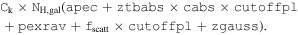
Figure 1 displays the X-ray images of NGC 3982, with the top row presenting all XMM-Newton camera images in the 0.3–10.0 keV band and the bottom row presenting the 3–78 keV images from each FPM camera on board NuSTAR. In all panels, the source+background extraction region is shown with a solid black line, whereas the background extraction regions are represented by dashed lines.
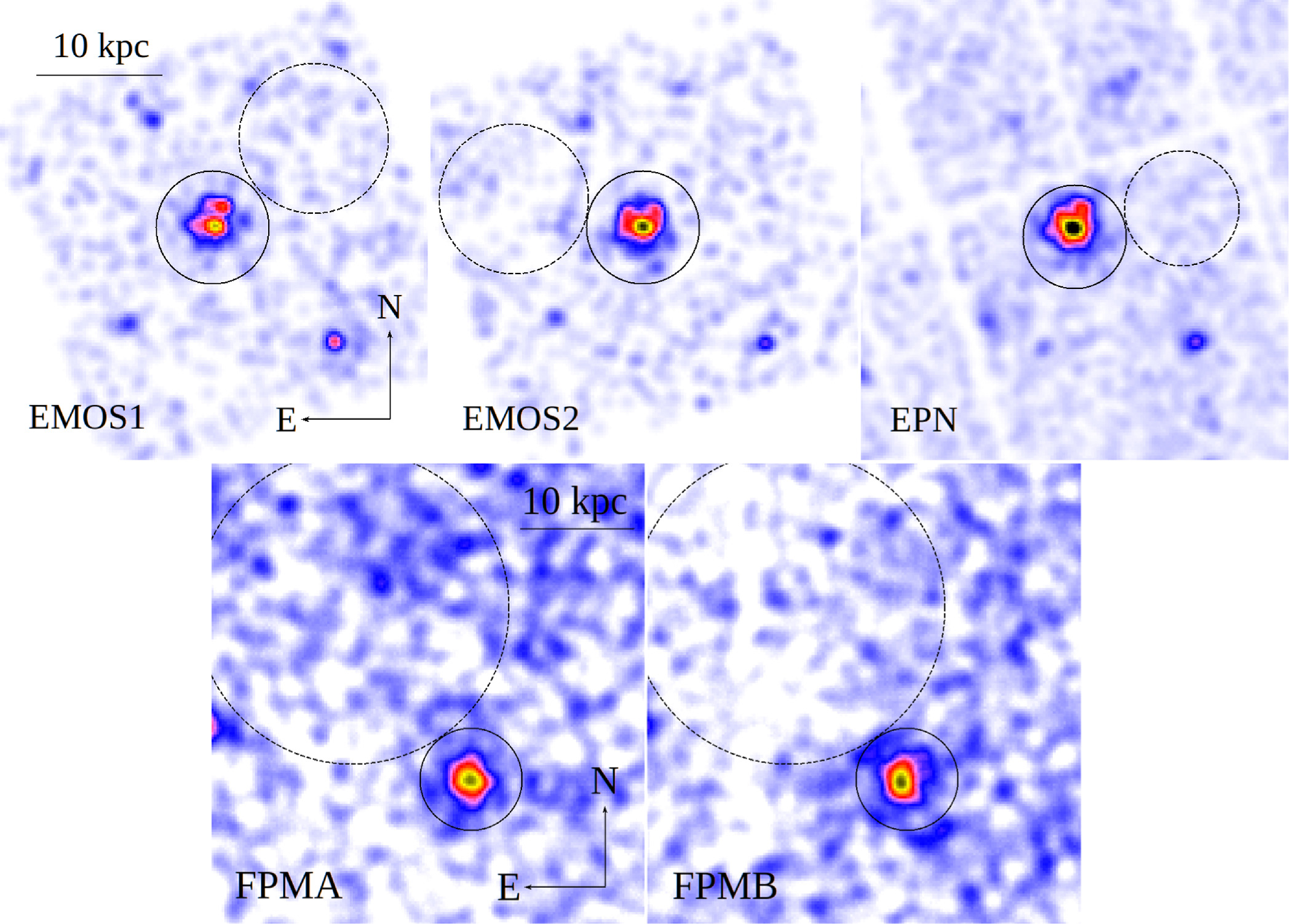
Figure 1. The 0.3–10.0 keV XMM-Newton (top) and 3–78 keV NuSTAR (bottom) X-ray images of NGC 3982 showing the extraction regions for source+background (solid circles) and background (dashed circles) spectra. The source+background regions have radii of 49'' for the EMOS and FPM detectors, and 45'' for EPN, due to the central readout node. The background regions have radii of 65'', 50'', and 150'' for the EMOS, EPN, and FPM detectors, respectively. The physical scale of 10 kpc corresponds to 1.8'.
Download figure:
Standard image High-resolution image3. X-Ray Spectral Fitting
The spectral analysis was performed for spectra binned using the ftgrouppha ftool, 10 such that each background spectrum would contain at least one count per bin, using the grouptype=bmin and groupscale=1 options. The Xspec package (Arnaud 1996) v12.12.0g was then used for spectral fitting with the modified Cash statistic (aka W-stat; Cash 1979; Wachter et al. 1979) invoked with the cstat command in Xspec. All data sets, including the three XMM-Newton spectra and the two NuSTAR spectra, were modeled simultaneously by tying all parameters, apart from a premultiplying cross-calibration constant.
All spectral fits in this paper used the Bayesian X-ray Analysis (BXA; Buchner et al. 2014) software package for global parameter estimation, unless otherwise stated. BXA connects the Xspec Python interface (PyXspec) with nested sampling algorithms that iteratively update the global parameter distribution initially defined by the user with parameter priors. As such, the algorithm is very effective at avoiding local minima and traversing toward the global statistical minimum associated with the model being fit to the data. BXA is thus also capable of reproducing complex interparameter dependencies and complex parameter posterior shapes that describe the multidimensional parameter constraints attainable with a given model. In this work, we use BXA v2.9 implemented with PyMultiNest (Buchner et al. 2014), the Python implementation of the nested sampling algorithm MultiNest (Feroz et al. 2009).
We performed the broadband X-ray spectral analysis in the energy range 0.3–10.0 keV for the XMM-Newton data and in 3–78 keV for the NuSTAR data by applying a variety of different spectral models, including both physically motivated models and the empirically motivated phenomenological model pexrav (Magdziarz & Zdziarski 1995). In the case of MYTorus, we performed the fitting starting at 0.6 keV, as this is the minimum energy allowed by the model.
For all models, the fixed parameters throughout the work are as follows. The multiplicative constant (C k), corresponding to the instrument cross-calibration, was initially left free to vary, to check for significant spectral offsets. No significant deviations from unity were found, such that the cross-calibration was frozen to unity in all subsequent fits, in agreement with the values found by Madsen et al. (2017). The redshift of NGC 3982 was frozen to 0.00371 (Martinsson et al. 2013), while the Galactic column density in the direction of the source (N H,gal) obtained from the nh tool was frozen to 1020 cm−2 (HI4PI Collaboration et al. 2016). For all models, we include an additional collisionally ionized apec model component to reproduce the soft excess emission ≲3 keV. The abundance of the apec component was set to solar, while the temperature and normalization were left free to vary, limited to the ranges [0.01, 5.0] keV and [10−8, 10−2] keV cm−2 s−1. The Thomson-scattered "warm mirror" emission was modeled as a fraction of the intrinsic power-law continuum (f scatt), representing a fraction of the coronal emission that passes through an obscurer with lower column density than the primary obscurer. The fraction is expected to account for ≲10% of the intrinsic X-ray continuum in obscured AGNs (Gupta et al. 2021). For all models where a cutoffpl component was used as the intrinsic continuum with variable high-energy cutoff, the value was frozen to 300 keV, in agreement with the value found by Baloković et al. (2020). For all free parameters discussed in Section 3, uniform or log-uniform priors were used, except for the photon index of the power-law component, where we defined a Gaussian prior with mean 2 and standard deviation 0.1, in agreement with previous results (Ricci et al. 2017a).
3.1. Pexrav
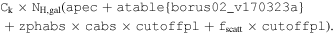
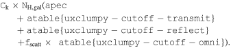
The phenomenological model pexrav (Magdziarz & Zdziarski 1995) assumes an intrinsic exponentially cutoff power-law spectrum reflected from a neutral semi-infinite slab. Such a geometry is not physically relevant for the obscurer in AGNs, since it does not account for transmission through the material nor for reprocessing from the obscurer. However, its inclusion provides an interesting comparison basis for the physical obscurer models we hitherto describe. In Xspec parlance, the model used was defined as:
The intrinsic obscurer 11 was described by the model components ztbabs × cabs, in which the column densities were tied and allowed to vary with a log-uniform prior between 1023 and 1026 cm−2. These two components reproduce the effects of photoelectric absorption and optically thin Compton scattering, respectively. We note that these model components are well known to struggle in accurately reproducing the predicted spectrum at high column densities (e.g., Yaqoob 1997), and such model limitations are exactly the scenarios we seek to compare with more appropriate physically motivated models. The Fe Kα line was modeled with a zgauss component with line energy and width frozen to 6.4 keV and 1 eV, respectively. The only free parameter for this component was hence the normalization. The photon index and normalization of the pexrav component were tied to the intrinsic continuum, while the cosine of the reflector inclination angle was left free to vary with a uniform prior in the range [0.10, 0.99]. The relative reflection fraction of pexrav (rel refl) was limited to negative values (to reproduce the pure reflection spectrum) with a log-uniform prior in the range [−100, − 0.01].
3.2. Borus02
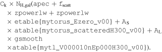
Borus02 is a physically motivated obscuring torus model based on the Monte Carlo radiative transfer simulations of Baloković et al. (2018). The geometry of the reprocessing medium is a uniform-density sphere, with two conical polar cutouts with variable half-opening angle to define the covering factor. The model was defined with the following expression:
We used the borus02 model in both coupled and decoupled modes. For borus02-coupled, all three column densities corresponding to the borus02, zphabs, and cabs components were tied together to vary log-uniformly in the range [1022, 1025.5] cm−2. The cosine of the inclination angle was left free to vary uniformly in the range [18.2, 84.3]°. For borus02-decoupled, the line-of-sight column densities of the zphabs and cabs components were tied together, but allowed to vary independently from the torus column density of the borus02 component. The inclination angle was frozen to ≈84° (see LaMassa et al. 2019 for more details of this setup). For both the decoupled and coupled model setups, the photon index and normalization of the different components were tied together and left free to vary. The covering factor (fC) of the obscurer was also allowed to vary uniformly over the range [0.1, 0.99].
3.3. MYTorus
MYTorus (Murphy & Yaqoob 2009) describes an obscurer with a uniform-density tube-like azimuthally symmetric torus corresponding to a classical "doughnut" geometry with a fixed opening angle of 60°. The model consists of three components, each represented with a different table model. These tables are the zeroth-order continuum component mytorus Ezero, the Compton-scattered continuum component mytorus scattered, and the fluorescence line emission mytl. We use the table models with a termination energy of ET = 300 keV and additionally include a Gaussian smoothing function for the fluorescent emission lines with the σL parameter via the gsmooth model component. The corresponding model expression was:
For MYTorus-coupled, we tied the photon index, normalization, equatorial column density, inclination angle, and intrinsic normalization between all three table models. The equatorial column density was left free to vary with a log-uniform prior in the range [1022, 1025] cm−2, while the cosine of the inclination angle was left free to vary uniformly within the range corresponding to [15, 89]°. The width of the Fe Kα line σL of the gsmooth component was frozen to 10−4 keV with the energy index α fixed to one.
3.4. UXCLUMPY
The Unified X-ray CLUMPY (UXCLUMPY) torus model is based on the Monte Carlo radiative transfer simulation code XARS
12
developed by Buchner et al. (2019). The geometry of this physically motivated table model is based on the clumpy torus model of Nenkova et al. (2008), with  spherical randomly distributed clouds. The obscurer column density is the highest in the equatorial plane, whereas the number of clouds along the line of sight for an edge-on system is
  . The number of clouds seen along the radial line of sight
  is axisymmetric and decreases with the inclination angle toward the poles. UXCLUMPY is the only model we employ that includes two distinct geometrical components. The torus dispersion of the main cloud population TORsigma effectively controls the torus scale height, and its cosine was allowed to vary uniformly in the range corresponding to [0, 84]°. An additional inner ring of dense Compton-thick clouds is included in UXCLUMPY that was found to have a significant effect on the observed Compton hump profile by Buchner et al. (2019). The CTKcover parameter describing the covering factor of that obscurer was allowed to vary uniformly in the range [0.1, 0.6].
The model setup is composed of three table models, corresponding to the transmitted and cold reflected components with fluorescent line emission and the warm mirror component (the "omni" component). The line-of-sight column density NH,los was allowed to vary log-uniformly in the range [1023, 1026] cm−2. The model expression was defined as:
The parameters of all table components were tied together and the inclination angle was allowed to vary in the range [0, 90]°.
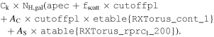
3.5. RXTorus
RXTorus is a physically motivated model by Paltani & Ricci (2017), generated with the RefleX platform, 13 a Monte Carlo code designed for tracking the propagation of individual X-ray photons through distributions of gas and dust. RXTorus is the first application of RefleX, adapting the same source and absorber geometries as MYTorus, while including the covering factor as a free parameter. The model consists of three table model components. RXTorus_cont_M is an exponential multiplicative tabular model for the continuum absorption component, where M denotes the metallicity (we assumed solar with M = 1). The reprocessed emission includes the Compton-scattered and fluorescent line emission and is given by the RXTorus_rprc_ M_CCC component, where CCC describes the high-energy cutoff. The model was defined using the following expression:
In RXTorus, the line-of-sight column density is defined by the following expression (Paltani & Ricci 2017):
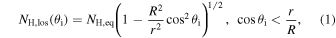
where θi represents the inclination angle and for  the line-of-sight column density is equal to zero. In our analysis, the equatorial column density NH,eq was left free to vary log-uniformly in the range [1023, 1025] cm−2. The ratio between the minor and major torus radii, r/R, represents the covering factor of the torus and was left as a free parameter to vary uniformly in the range [0.1, 0.8], while the inclination angle was allowed to vary in the range [20, 89]°. All parameters were tied between individual table models, and the intrinsic continuum assumed an exponential cutoff energy of 200 keV.
4. Results
Initially we fit the broadband X-ray spectra with the default minimization algorithm available in Xspec (the Levenberg–Marquardt algorithm; Levenberg 1944; Marquardt 1963), which converges toward a minimum using local information from the surrounding parameter space, starting at an initial parameter guess. The fit with the UXCLUMPY model obtained within Xspec is shown in Figure 2, together with the corresponding residuals (bottom left panel) and the residuals obtained for all the different models tested here (right panels). A visual comparison of the residuals shows how indistinguishable the model fits are for all data sets. Similarly the fit statistics (C/dof) listed in Table 1 show that the fits are comparable among all models. However, the derived posteriors for some of the parameters varied dramatically among different models. For instance, we found large discrepancies between the derived scattering fraction, ranging from 0.01% found by borus02-decoupled up to 10% estimated by pexrav. The rest of the models predict a scattering fraction in range 0.1%–0.5%. The covering factor and the inclination angle were also found to differ dramatically by different models, predicting the opening angle in a range from 60° up to 84° and the inclination from 21° up to an almost edge-on system. On the other hand, the column density for most of the models was found to be pegged to the upper limits defined by the specific model, suggesting the Compton-thick nature of NGC 3982. The fundamental reason for such differences is the ability of models to reproduce the same spectral shapes with unique parameter combinations.
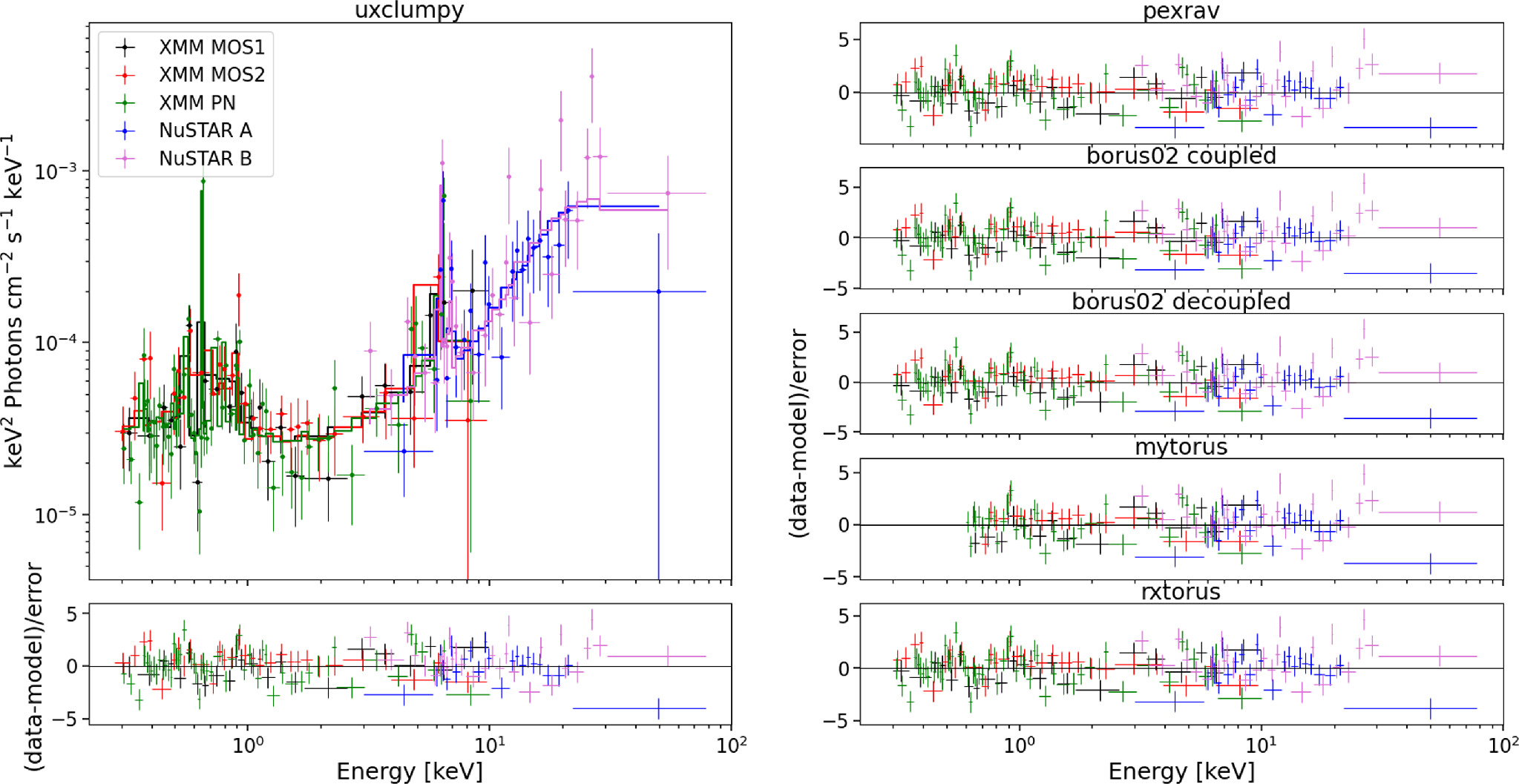
Figure 2. The XMM-Newton and NuSTAR spectra modeled and unfolded with UXCLUMPY model (top left) with corresponding residuals (bottom left) and residuals for the rest of the tested spectral models (right) described in Section 3.
Download figure:
Standard image High-resolution imageTable 1. Posterior Parameter Constraints with All Uncertainties Corresponding to 68% Confidence Level
| Component | Parameter | Unit | pexrav | borus02 c. | borus02 d. | MYTorus | UXCLUMPY | RXTorus |
|---|---|---|---|---|---|---|---|---|
| apec |

| erg s−1 |

|

|

|

|

|

|
| SFRX-ray | M⊙ yr−1 |

|

|

|

|

|

| |
| Torus Properties |

| cm−2 |

|

|

|

|

|

|

| cm−2 | ⋯ | ⋯ |

|

| ⋯ |

| |
| fC | ⋯ | ⋯ |

|

| 0.5 a |
 b
b
|

| |
| θhalf-opening | deg | ⋯ |

|

| 60 a |
 b
b
|

| |
| θinclination | deg |

|

| 84.3 a |

|

|

| |
| Scattering Fraction | fscatt | % |

|

|

|

|

|

|
| Power Law | Γ | ⋯ |

|

|

|

|

|

|
| log K | keV cm−2 s−1 |

|

|

|

|

|

| |
| AGN Properties |

| erg cm−2 s−1 |

|

|

|

|

|

|

| erg cm−2 s−1 |

|

|

|

|

|

| |

| erg s−1 |

|

|

|

|

|

| |

| erg s−1 |

|

|

|

|

|

| |

| erg s−1 |

|

|

|

|

|

| |

| erg s−1 |

|

|

|

|

|

| |
| λEdd | % |

|

|

|

|

|

| |
| Fit Statistic | C/dof | ⋯ | 2354.9/2877 | 2351.0/2877 | 2351.7/2877 | 2277.8/2808 | 2352.1/2876 | 2352.3/2877 |

| ⋯ | −1190.4 | −1186.3 | −1190.4 | ⋯ | −1185.7 | −1188.3 | |
Notes. u: the uncertainty is unconstrained, as the fit is pegged to the hard limit.
a Fixed for the modeling. b Estimated by linear grid interpolation using TORsigma and CTKcover for .
.Download table as: ASCIITypeset image
We next performed the analysis using BXA for all the described models. Results from the global parameter estimation, showing the median and uncertainties at the 68% confidence level of the posterior estimates, are shown in Table 1, together with the Bayesian global evidence ln Z. All models describe the observed spectra similarly well, though we note the Bayesian evidence for MYTorus is not listed, since we fit this model to data with energy E > 0.6 keV. Corner plots displaying all posterior probability distributions obtained by BXA are shown in the Appendix.
There is broad agreement between the line-of-sight column densities derived by the different models, all of them resulting in NH > 1.5 × 1024 cm−2 to >99% confidence, thus confirming the Compton-thick nature of the circumnuclear obscurer in NGC 3982. The equatorial column density in both MYTorus and RXTorus and the global column density in borus02-decoupled were pegged to the maximum value allowed for this parameter.
While the covering factor of the coupled MYTorus model is fixed to a value of 0.5 (i.e., a half-opening angle of 60°), this parameter was free in the other models. For RXTorus, we found a covering factor of 0.47 ± 0.12, corresponding to a half-opening angle of 62° ± 8°. For the UXCLUMPY model, we found TORsigma =  and the Compton-thick covering factor of the inner ring CTKcover = 0.2 ± 0.1. Owing to the probabilistic generation of clouds from a distribution (Buchner et al. 2019), the covering factor in UXCLUMPY is difficult to analytically define. We estimated the covering factor using a precomputed grid of TORsigma, CTKcover, and a covering factor for sightlines with log NH > 24 (Boorman et al. 2023). We used a grid interpolator on a random sample of UXCLUMPY posterior rows to produce a posterior on the covering factor given by fC ≈ 0.5 ± 0.1, which is fully consistent with the values found by the other models (see Figure 3).
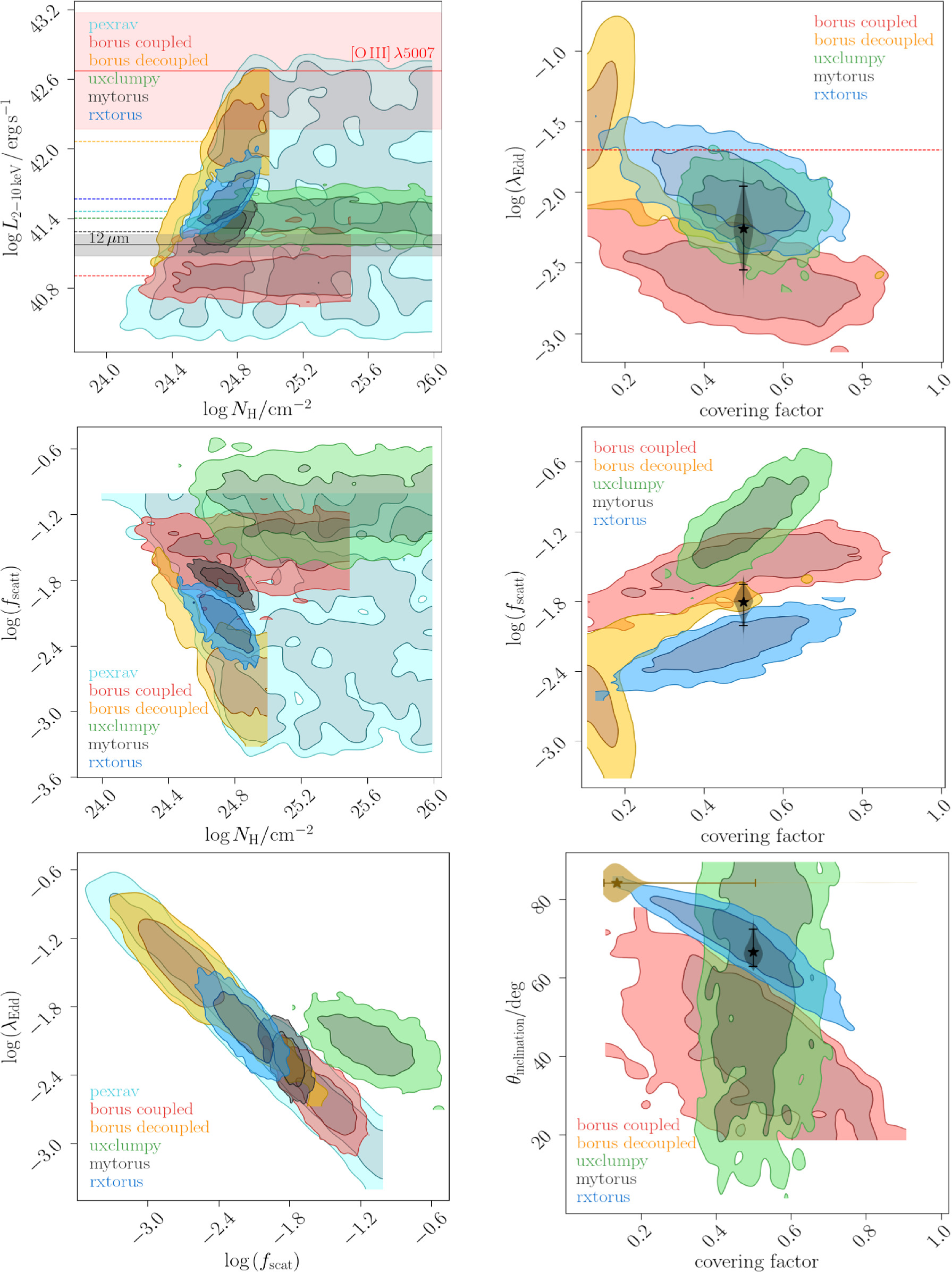
Figure 3. Contour plots for different posterior combinations. Top left panel: X-ray luminosity in the 2-10 keV band as a function of the column density. The black and red solid lines represent the 50th quantile of the intrinsic luminosity derived from Equations (2) and (3), respectively, with the shaded regions corresponding to the 16th and 84th quantiles of the distributions. The dotted line shows the median luminosity for different models. Right panels: Eddington ratio (top right), scattering fraction (middle right) and inclination angle (bottom righ) as a function of the covering factor of the torus. The MYTorus model has the covering factor fixed, and the corresponding Eddington ratio distribution is shown with the violin plot, while the star indicates the median and the error bars indicate 2σ uncertainties. Similarly, in the bottom right panel, the inclination angle for borus-decoupled is fixed, so the corresponding covering factor distribution is shown with a violin plot and a 2σ error bar. Top right panel: the red dashed line represents the effective Eddington limit for a dusty gas (Ricci et al. 2017c). Middle left panel shows the scattering fraction as a function of the column density while bottom left panel displays the Eddington ratio as a function of the scattering fraction. The different contours show the 1σ and 2σ uncertainties.
Download figure:
Standard image High-resolution imageWe find that for borus02-coupled, the preferred inclination angle is smaller than the half-opening angle of the torus at the 3σ confidence level, which might suggest an unobscured source. However, the line-of-sight component of this model is not dependent on the inclination angle or on the very high global column density (≈1025 cm−2). An inclination angle smaller than the half-opening angle could suggest a scenario in which the spectrum is dominated by reflection from the back wall of the torus, in favor with the reflection-dominated broadband spectrum. On the other hand, for borus02-decoupled, we obtain an upper limit of the covering factor (fC ≲ 0.17). This indicates that the fit favors a dense low covering obscurer, possibly resembling a disk-like structure. It should be noted, however, that this might also be caused by our assumption that the inclination angle corresponds to an edge-on system. Additionally, further uncertainties may arise from an error in the Green functions associated with borus02, as reported by Vander Meulen et al. (2023), though we note the line-of-sight column density contours from borus02 are in good agreement with with the other models.
4.1. Intrinsic AGN Luminosity and Eddington Ratio
The posterior values of the photon index and power-law normalization were used to determine the intrinsic luminosity with the Hubble distance corrected to the reference frame defined by the 3K cosmic microwave background, 18.91 Mpc. 14 The observed median 2–10 keV luminosity was found to be ≈(4.6–5.9) × 1039 erg s−1 across different models. We further estimated the intrinsic X-ray luminosity in two different energy bands, 2–10 keV and 8–24 keV, respectively, as listed in Table 1. The intrinsic luminosity of borus02-coupled was found to have the lowest median value, L2–10 keV ≈ 8 × 1040 erg s−1, which was up to 2 orders of magnitude lower than the highest one found by borus02-decoupled, with median L2–10 keV ≈ 1 × 1042 erg s−1. However, for the majority of the models, the median 2–10 keV intrinsic luminosity was found to be in the range ≈(1.9–3.7) × 1041 erg s−1.
The Eddington ratio (λEdd) is an important parameter, as it traces the growth rate of SMBHs. It is given as a fraction of the bolometric luminosity and the Eddington luminosity, λEdd = Lbol/LEdd ∼ Lbol/MBH, where MBH is the mass of the SMBH. We calculated the bolometric luminosity of NGC 3982 using the 2–10 keV band luminosity, adopting the X-ray bolometric correction for Compton-thick AGNs from Brightman et al. (2017),  . The Eddington luminosity was derived via the black hole mass given in (Kammoun et al. 2020;
  ), which was calculated from the M–σ relation from Kormendy & Ho (2013). We included an additional 0.5 dex uncertainty for all subsequent Eddington ratio estimations. The median Eddington ratios we find encompass the range ≈0.2%–1.1% for most of the models, but for pexrav and borus02-decoupled, the estimated Eddington ratio posteriors cover substantially larger ranges, as high as 6% at the 68% confidence level. Both bolometric luminosities and Eddington ratios for all models are listed in Table 1.
Regarding the soft X-ray band, all models found very similar values for the temperature and normalization of the apec component. The temperature was found to be ≈0.28 keV for the majority of the models with a median normalization in the range ≈(4.2–4.5) × 10−5 keV cm−2 s−1. Only MYTorus-coupled found slightly higher temperatures of 0.33–0.43 keV and median normalization ≈2.9 × 10⁻⁵ keV cm−2 s−1, though it is important to stress that MYTorus is limited in the soft X-ray band to energies >0.6 keV. We further estimated the intrinsic soft X-ray luminosity in the 0.5–2.0 keV band from the apec component to derive the host galaxy star formation rate, using Equation (2) in Mineo et al. (2012). We note that Mineo et al. (2012) calculated luminosities with mekal, though the differences with our apec-based measurements should be minimal, given the statistical uncertainty of the data being fit. The soft X-ray luminosity derived from the apec model component was found to be ≈(3.2 ± 0.3) × 1039 erg s−1, while the corresponding star formation rates were found to be ≈6 ± 2 M⊙ yr−1 for the majority of the models. The MYTorus model predicts a slightly smaller luminosity of ≈(2.6 ± 0.3) × 1039 erg s−1, corresponding to a predicted star formation rate of ≈5 ± 2 M⊙ yr−1. These results are consistent within uncertainties with findings of Lianou et al. (2019), who estimated a global star formation rate of ≈2.9 ± 2.7 M⊙ yr−1, using the WISE 22μm band corrected for the emission of evolved stars.
5. Discussion and Future Prospects
Given the majority of the AGNs in the Universe are obscured (Buchner et al. 2014; Ueda et al. 2014; Brandt & Alexander 2015; Ricci et al. 2017a), to understand the bulk of AGNs we need to fully comprehend the intrinsic properties of those systems that are deeply buried in thick layers of dust and gas. By exploring the posterior parameter space of a Compton-thick low-luminosity AGN with different physically motivated models, we can quantify how well different parameters of interest can be estimated reliably in low-flux targets.
The model posterior distributions obtained via global parameter estimation with BXA were used to visualize the corresponding parameter spaces of each model in Figure 3. Some models are seen to cover very large ranges, e.g., pexrav, which covers a range of ∼2 dex for both intrinsic luminosity and line-of-sight column density. In some cases, different geometries predict very different overall values for a given parameter, e.g., for borus-coupled, 72% of the posterior intrinsic luminosity points are below 1041 erg s−1, but for pexrav this is only 29%, and other models predict the intrinsic luminosity to be higher than 1041 erg s−1 with >99% probability. Similarly, regarding the scattering fraction, borus-decoupled and RXTorus predict the fraction of the scattered light to be smaller than 1% with >86% probability. On the other hand, borus-decoupled, MYTorus, and UXCLUMPY predict a scattering fraction higher than 1% with >97% probability, while for pexrav this value is close to the median of the distribution.
5.1. Mid-infrared and Optical Emission
The intrinsic AGN X-ray luminosity can also be estimated by looking at the emission in other "isotropic" wavelengths. For example, the primary radiation of an AGN can be reemitted in the mid-infrared (MIR) wave band after being reprocessed by hot dust. The monochromatic 12 μm MIR luminosity is therefore found to be tightly correlated with the 2–10 keV X-ray luminosity (Elvis et al. 1978; Glass et al. 1982; Krabbe et al. 2001; Lutz et al. 2004; Almeida et al. 2007; Gandhi et al. 2009; Asmus et al. 2015). To estimate the intrinsic X-ray luminosity from the nuclear MIR dust emission, we adopted the following relation from Asmus et al. (2015):
Here,  and
and  represent the luminosity in units of 1043 erg s−1. Similarly, the correlation between the X-ray 2–10 keV and optical [O iii] λ5007 emission has also been well explored (Ward et al. 1988; Panessa et al. 2006; González-Martín et al. 2009; Berney et al. 2015), connecting the emission of the central regions to the extended partially ionized narrow-line region. We adopted the relation between the optical [O iii] λ5007 and 2–10 keV X-ray luminosity from Berney et al. (2015):
However, we note the [O iii] can be strongly affected by variability, as it traces the power of the central engine in the past, as well as host galaxy contamination, which can lead to substantial scatter (e.g., Ueda et al. 2003). We therefore obtain a complementary estimate of the X-ray luminosity of NGC 3982 by using both optical [O iii] λ5007 and MIR 12 μm observations.
15
The nuclear MIR luminosity of NGC 3982,  , was adopted from Asmus et al. (2015), and the [O iii] λ5007 luminosity of NGC 3982,
 ![$\mathrm{log}{L}_{[{\rm{O}}\,{\rm\small{III}}]}=40.50$](https://content.cld.iop.org/journals/0004-637X/966/1/116/revision1/apjad3235ieqn116.gif) , corrected for Galactic absorption and narrow-line region extinction, was adopted from Panessa et al. (2006). The estimated 2–10 keV luminosities using Equations (2) and (3) are plotted as horizontal lines with associated 68% interquartile shaded ranges in the top left panel of Figure 3.
, corrected for Galactic absorption and narrow-line region extinction, was adopted from Panessa et al. (2006). The estimated 2–10 keV luminosities using Equations (2) and (3) are plotted as horizontal lines with associated 68% interquartile shaded ranges in the top left panel of Figure 3.
The [O iii] λ5007 emission predicts  . As is notable from the top left panel of Figure 3, we find a significantly lower intrinsic X-ray luminosity for most of the models, despite the large uncertainties arising from the adopted correlation.
16
This suggests that the AGN might have been more active in the past, hence the higher X-ray luminosity inferred from the extended [O iii] emission. This finding is in agreement with the discovery of Esparza-Arredondo et al. (2020), who identified NGC 3982 as a fading AGN candidate. On the other hand, from the MIR-versus-X-ray luminosity correlation, we found
. As is notable from the top left panel of Figure 3, we find a significantly lower intrinsic X-ray luminosity for most of the models, despite the large uncertainties arising from the adopted correlation.
16
This suggests that the AGN might have been more active in the past, hence the higher X-ray luminosity inferred from the extended [O iii] emission. This finding is in agreement with the discovery of Esparza-Arredondo et al. (2020), who identified NGC 3982 as a fading AGN candidate. On the other hand, from the MIR-versus-X-ray luminosity correlation, we found  . This value is reproduced by all the tested models within 2σ uncertainties, but we note some (e.g., borus-decoupled and pexrav) cover a very large range of predicted X-ray luminosity. In estimating the X-ray luminosity, the nuclear 12 μm emission is more precise than the [O iii] line emission, since the MIR-versus-X-ray relation has lower overall observed scatter. In addition, the MIR emission is likely being emitted from closer regions to the central engine than the [O iii] emission arising on larger narrow-line region scales, and so may be less affected by host galaxy contamination. Future multiwavelength physically motivated obscurer models such as those attainable with RefleX and SKIRT (e.g., Andonie et al. 2022; Ricci & Paltani 2023; Vander Meulen et al. 2023) would hence be useful in defining multiwavelength prior constraints on the intrinsic AGN power derived in X-ray spectral fitting.
5.2. Unique Model Dependencies
As NGC 3982 is a low-flux source, the uncertainties of the posterior parameters are large, as illustrated in Figure 3. Even though the derived distributions cover similar ranges of parameter values (e.g., the lower limit of the column density is in agreement for all models), the shapes of the distributions in all the 2D posterior parameter spaces considered in Figure 3 differ significantly. The distributions in the top left panel of Figure 3 illustrate how for a higher column density a larger intrinsic luminosity is needed. This is expected, as for more luminous sources, a higher line-of-sight column would be required to reproduce the same observed flux. The right panels of Figure 3 show the parameter posterior dependencies between the covering factor and intrinsic power propagated into the Eddington ratio, scattering fraction, and inclination angle, which are found to be somewhat degenerate across all models. Overall, the covering factor is only poorly constrained with large uncertainties for all models, showing how difficult it can be to estimate the geometry of the obscurer from X-ray spectral fitting in the low-count regime. The top right panel shows that NGC 3982 is predicted to be below the effective Eddington limit for dusty gas (the red dotted line is from Ricci et al. 2017c) by the majority of the models, as expected for high column densities of circumnuclear gas. As illustrated in the bottom right panel, the inclination angle for UXCLUMPY was not constrained, but we found a strong degeneracy between the inclination angle and the covering factor for RXTorus, since larger covering factors can accommodate smaller inclination angles while still being obscured. A similar trend is seen with borus02 through borus-coupled, with much larger uncertainties. Regarding the scattering fraction, we found a large range of posterior parameter values between different models, predicting fscatt as low as  % for pexrav and
  % for borus-decoupled, up to
  % as estimated by UXCLUMPY. The bottom left panel shows a strong degeneracy between the scattering fraction and the Eddington ratio, likely due in part to the difficulty associated with constraining the intrinsic normalization in reflection-dominated spectra. UXCLUMPY shows a deviation from the other models, giving higher Thomson-scattered fractions when compared with the intrinsic accretion power on average. A plausible reason for this deviation is the treatment of the warm mirror component in our UXCLUMPY model setup, as compared to the other models we consider. We use the physically motivated "omni"-directional warm mirror component (see Section 4.3 of Buchner et al. 2019) that describes warm Compton scattering from the intercloud volume-filling gas as well as cold Compton scattering from the dense clouds. To first order, the warm mirror component with this method is a power law. But the overall Thomson-scattered flux arising from a given fraction will be lower (for a given intrinsic coronal flux) than for the simpler formalism employed in the other model setups, on average.
Overall, Figure 3 shows that different models can produce posterior distributions with significantly different shapes and even predict discrepant posterior parameter ranges. The corresponding posterior model spectral realizations associated with these unique posterior distributions are shown in Figure 4 to have very similar spectral shapes up to ∼30 keV. Above this energy, the spectral curvature of the Compton hump from each model is somewhat unique for each torus geometry, but the data in this energy range are insufficient to constrain any model parameters from them. Future higher-S/N broadband spectra and/or high-spectral-resolution X-ray observations together with next-generation physical models will hence help to reliably distinguish between different torus geometries (see Section 5.4).
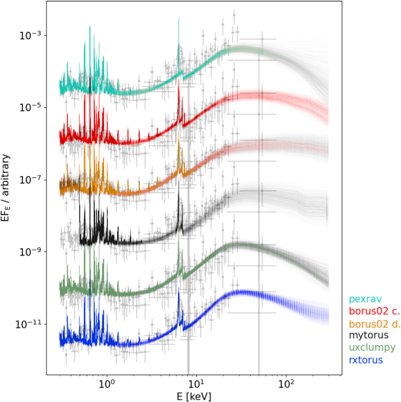
Figure 4. Posterior model realizations plotted over the spectral data unfolded with a Γ = 2 power law are shown in gray. The overall spectral shapes predicted by each model are very similar up to ∼30 keV (further supported by the similar C/dof in Table 1), with spectral differences predicted above this value. Future high-sensitivity broadband spectroscopy including E > 30 keV will hence be key to distinguishing geometric models of the obscurer via the shape of the Compton hump.
Download figure:
Standard image High-resolution imageStudying obscured AGNs down to low luminosities is important for understanding the bulk of the AGN population, as they likely form a large fraction of AGNs. Many AGN population synthesis models predict that a large fraction of Compton-thick AGNs will be necessary to reproduce the observed spectral shape of the cosmic X-ray background (e.g., Gilli et al. 2007; Treister et al. 2009; Akylas et al. 2012; Comastri et al. 2015). However, many heavily obscured AGNs harboring a moderately accreting SMBH are beyond our capabilities for detection with current X-ray observatories, even in the local Universe at distances just above ∼50–100 Mpc (e.g., Ricci et al. 2015). NGC 3982, for example, would most probably remain undetected in NuSTAR observations if located as far as ∼40 Mpc, roughly double its Hubble distance. We also expect many heavily obscured moderately accreting SMBHs at the peak of the star formation and black hole growth at redshift z ∼ 2 (e.g., Ueda et al. 2014). Such sources could be significantly contributing to the cosmic black hole growth while still remaining hidden behind layers of gas and dust.
5.3. Local versus Global Parameter Exploration
To quantitatively evaluate the performance of the local parameter exploration with Xspec in comparison with the global parameter exploration from BXA, we performed Monte Carlo simulations. We loaded the corresponding model spectral realization associated with each posterior model row in Xspec, as an initial position of parameter space that was by definition close to the global minimum found by BXA. We then ran Levenberg–Marquadt-based X-ray spectral fits from these starting positions many times, tracking the best-fit parameter values acquired in each iteration. Although the exact number of realizations varies from model to model, they all fall in between 2226 and 3093.
Examples of a selection of interesting parameter distribution comparisons for MYTorus and UXCLUMPY are shown in Figure 5, where we reiterate that the BXA posterior distribution illustrated in blue was used on average as the prior parameter guess for each Xspec fit used to generate the corresponding orange distributions. All the orange parameter distribution shapes are significantly different from those found with BXA. Some parameter distributions are clearly consistent with the local parameter exploration algorithms getting stuck in local minima (e.g., photon index and scattered fraction), where the mode that is consistent with BXA is of significantly lower probability than a secondary mode that is entirely inconsistent with BXA. Other parameters (e.g., line-of-sight column density and inclination angle) are broadly consistent with the average distribution found with BXA, though with additional probability weight located at the extremes of the BXA distributions. The discrepancies we find from fitting with local parameter exploration imply that X-ray spectral fitting can be significantly affected by local minima, though we note that our local parameter estimates do not consider their associated errors, which could lead to more overall consistency with BXA. A full quantitative comparison between global and local parameter explorations would require comprehensive simulations of different parameter values, which is outside the scope of the current work.
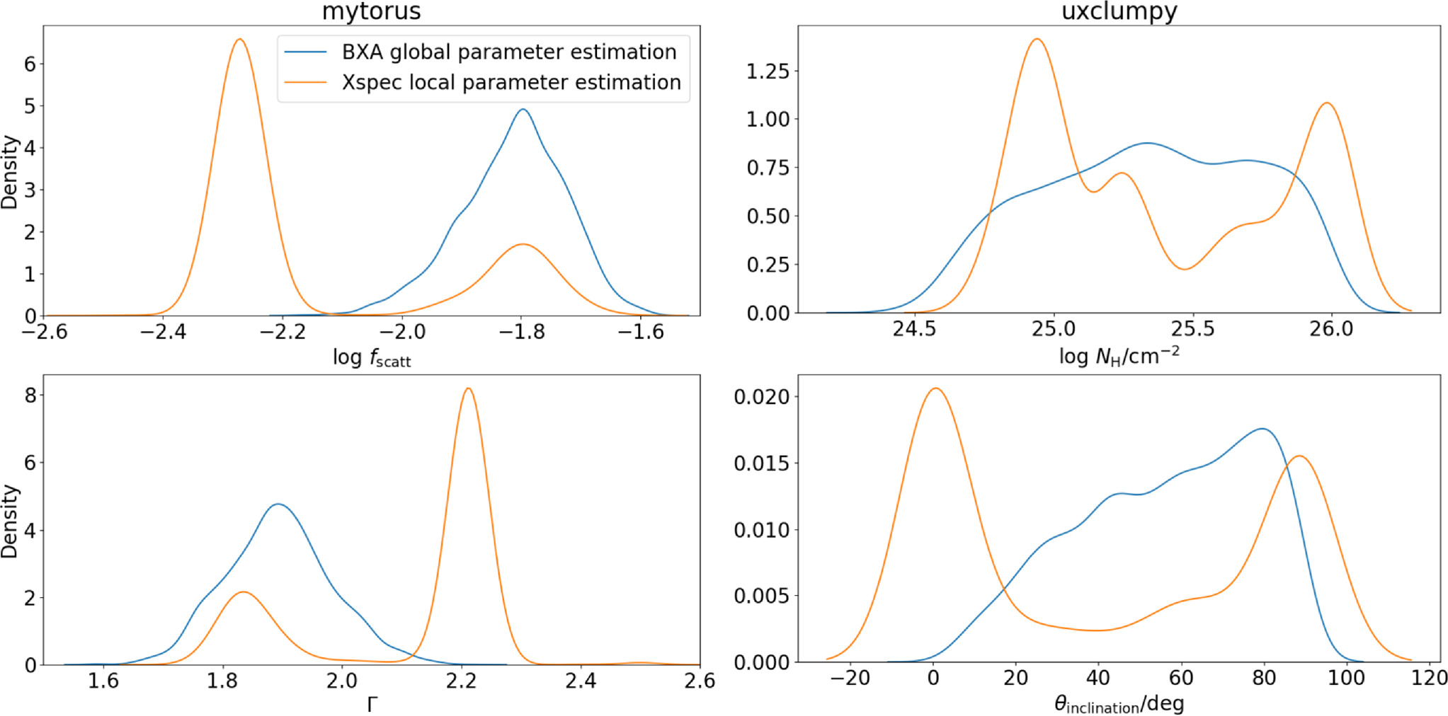
Figure 5. The posterior parameter distributions for the logarithm of the scattering fraction (log fscatt) and the photon index (Γ) obtained by the MYTorus model (left panels) and the logarithm of the line-of-sight column density (logNH) and the inclination angle (θinclination) for the UXCLUMPY model (right panels). The posterior values from BXA (blue) were used to inform the initial parameter values used in the local parameter exploration with Xspec. The distributions of the best-fit values originating from the local parameter estimation in Xspec are shown in orange. All distributions shown are generated with a kernel density estimate approximation to the actual distributions, which is why, for example, the inclination angle distributions appear to allow negative values that are not attainable in any of the models tested.
Download figure:
Standard image High-resolution image5.4. HEX-P Simulations
HEX-P 17 (Madsen et al. 2024) is a next-generation probe-class mission concept that provides simultaneous broadband coverage (0.2–80 keV) via the combination of two hard-X-ray-focusing high-energy telescopes (HETs) and a low-energy telescope, with significantly improved sensitivities relative to XMM-Newton and NuSTAR combined. Here we visualize the spectral improvements attainable with HEX-P in studying the circumnuclear obscurers in the bulk of the Compton-thick AGN population, by running spectral simulations from our spectral fits to NGC 3982. We note that the HEX-P simulations shown are conservative, since NGC 3982 is one of the lowest-luminosity Compton-thick AGNs known within a volume of ∼20 Mpc.
The HEX-P response files, version v07, for the two HETs on board HEX-P were used to simulate broadband spectra, where we focused on the 2–80 keV energy band for visualization. The simulations were performed from our BXA UXCLUMPY best-fit model, with nine different combinations of TORsigma and CTKcover to test a wide number of geometrically distinct configurations for the obscurer. For TORsigma, we assumed values of 7°, 28°, and 84°, and for CTKcover, we used 0.0, 0.3, and 0.6, with a total exposure of 200 ks. The inclination angle was fixed to 70°, while the line-of-sight column density was set to 4.2 × 1025 cm−2. To aid comparison, we performed the same spectral simulations, with the response and background files from the real NuSTAR/FPMA observation and with the same exposure as for HEX-P.
Figure 6 shows both the NuSTAR and HEX-P simulated spectra, normalized to unity at 7.1 keV, to show the range in Compton hump shapes expected from the different obscurer geometries described by TORsigma and CTKcover. As Figure 6 illustrates, HEX-P is capable of constraining not only the spectral shape <30 keV, which is key for measuring column density and inferring intrinsic AGN parameters, but also the geometrical properties of their circumnuclear obscurers, from distinct Compton hump shapes. Such studies with HEX-P will thus open up a new era for understanding the connection between the intrinsic properties of the central source and the obscurer in heavily obscured AGNs, down to low intrinsic AGN powers. Such a connection is currently difficult to constrain in Compton-thick AGNs, as compared to the less obscured AGN population (e.g., Ricci et al. 2017c).
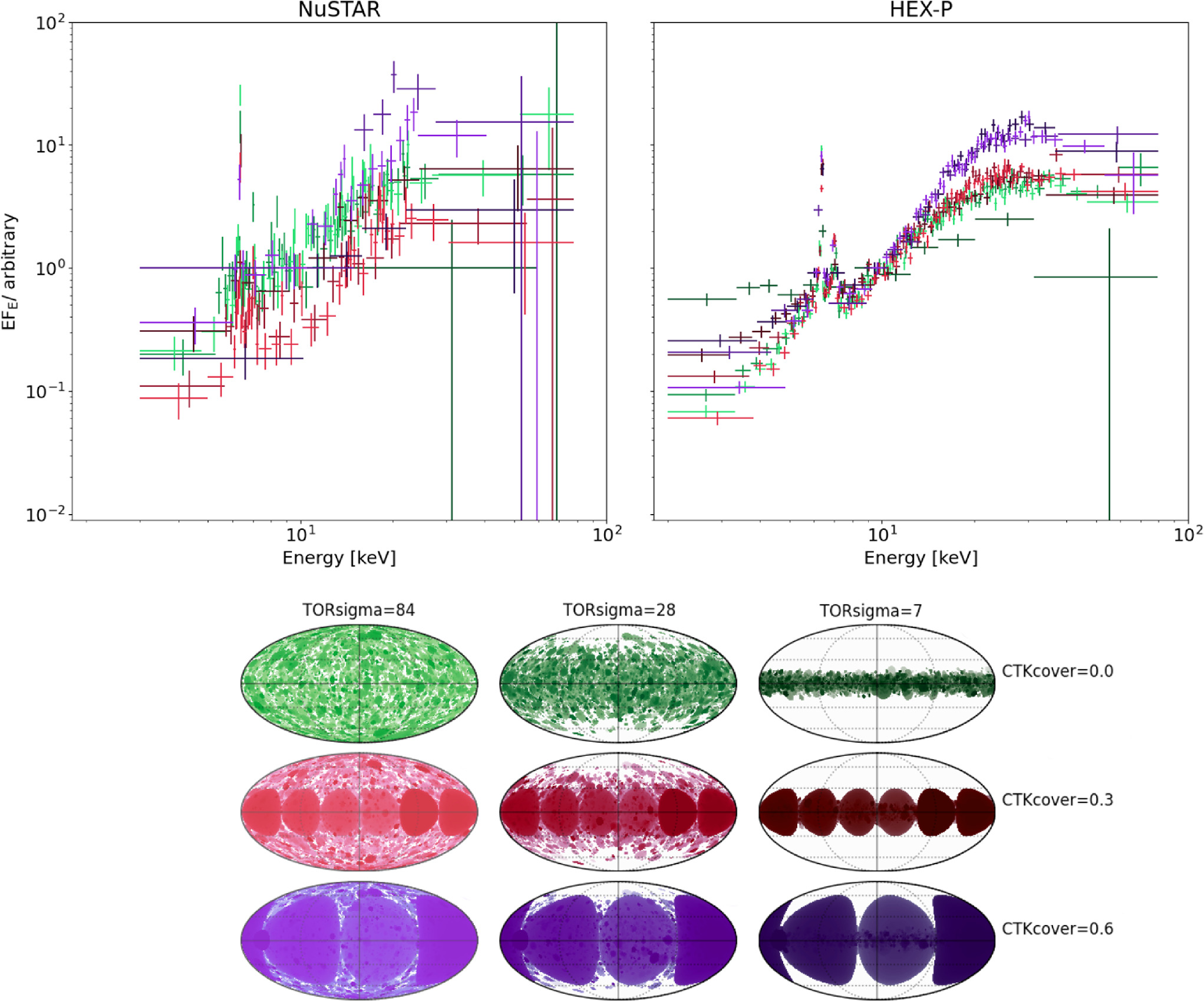
Figure 6. NuSTAR spectra simulated using the UXCLUMPY model (left) using an exposure of 200 ks and for nine different combinations of TORsigma and CTKcover. Equivalent simulations for HEX-P (right) allow the identification of differences in the Compton hump shape arising from different obscurer geometries. The colors indicate different combinations of TORsigma and CTKcover describing the geometry of the obscurer in UXCLUMPY, as illustrated by the obscurer maps in the bottom panel. The maps are adopted from the UXCLUMPY GitHub page (https://github.com/JohannesBuchner/xars/blob/master/doc/uxclumpy.rst).
Download figure:
Standard image High-resolution image6. Summary and Conclusion
This work investigates the model–parameter dependencies arising from a detailed analysis of the X-ray spectral properties of the low-luminosity Seyfert 2 AGN NGC 3982. We fit the broadband X-ray spectra generated from XMM-Newton and NuSTAR with five different obscurer models, using local and global parameter exploration algorithms. Our key findings are:
- 1.Compton-thick classification. The line-of-sight column density was found to be >1.5 × 1024 cm−2 for all the models at the 3σ confidence level, reaching values as high as log NH/cm−2 = 24.9–25.8 for uxclumpy (see Table 1). We thus confirm NGC 3982 to be a Compton-thick AGN.
- 2.Interparameter dependencies. The 2D posterior parameter distributions acquired with BXA show clearly different shapes across the models considered (see Figure 3), even though some of the 1D parameter distributions are comparable. We find a large range of predicted intrinsic luminosities, highlighting the difficulties associated with constraining the intrinsic continuum in reflection-dominated Compton-thick AGNs.
- 3.Intrinsic AGN power. We compare the intrinsic X-ray luminosity predicted to bolometric indicators of intrinsic AGN power. The median X-ray luminosity in the 2–10 keV band was found to be 1040.9–42.1 erg s−1 for individual models (see Table 1), which is in agreement with estimations from the MIR 12 μm emission at the 68% confidence level for all models considered (see the top left panel of Figure 3). On the other hand, we predicted a much higher X-ray luminosity from the optical [O iii] λ5007 emission, potentially indicating the source was more luminous in the past, in agreement with Esparza-Arredondo et al. (2020). The Eddington ratio was found to be below the dusty gas limit found by Ricci et al. (2017c) for all the models (see the top right panel of Figure 3), with the majority of models predicting a posterior median Eddington ratio in the range 0.2%–1.1%.
- 4.Predicted spectral shapes. Despite each model reproducing unique multidimensional parameter posterior distributions, we found the corresponding model realizations to have very similar spectral shapes up to ∼30 keV, as shown in Figure 4. We additionally found the critical energy region for distinguishing models is E ≳10 keV, in which the current spectral constraints are insufficient.
- 5.Local versus global parameter exploration. We perform Monte Carlo tests comparing local to global parameter exploration, finding that local parameter estimation can give clearly different results from global parameter estimation techniques for specific parameters (see Figure 5). This shows the advantages of algorithms—such as those available with BXA—in fitting complex models, in addition to the low-flux regime.
- 6.HEX-P. By simulating HEX-P spectra of NGC 3982, we show the benefits of simultaneous high-sensitivity broadband X-ray spectroscopy in disentangling multiple spectral components >10 keV. HEX-P, in combination with complex future torus models, will hence constrain the geometrical and physical properties of the circumnuclear obscuring material in the low-luminosity Compton-thick AGN population as well as its connection with intrinsic AGN characteristics.
Our study highlights that X-ray spectral fitting of obscured AGNs not only relies on the data being fit and the method used to perform the fitting, but also, inherently, on the choice of model. Using global parameter exploration algorithms to fit multiple models is a powerful method of quantifying the effects model dependencies have on deriving the key parameters from obscured AGNs.
Acknowledgments
The authors are grateful to the referee for helpful comments. K.K. and C.R. acknowledge support from ANID BASAL project FB210003. P.B. acknowledges financial support from the Czech Science Foundation under Project No. 22-22643S. C.R. acknowledges support from Fondecyt Regular grant 1230345.
Appendix: Posterior Probability Distributions
This section presents the posterior probability corner plots in Figures 7, 8, 9, 10, 11, and 12 for pexrav, borus02-coupled, borus02-decoupled, mytorus, uxclumpy, and rxtorus, respectively, giving the 1D and 2D marginalized posteriors for all the fitted parameters showing 5σ intervals, with uncertainties marked by dashed lines indicating the 95% (2σ) interval.

Figure 7. Posterior probability distributions for the pexrav model. The parameters in the columns (rows) are displayed as follows, from left to right (top to bottom): (1) logarithm of the intrinsic column density in units of 1022 cm−2; (2) photon index; (3) logarithm of the power-law normalization; (4) negative value of the logarithm of the relative reflection; (5) cosine of the inclination angle; (6) logarithm of the scattering fraction; (7) logarithm of the apec temperature in kiloelectronvolts; (8) logarithm of the apec normalization; and (9) logarithm of the fluorescent Fe Kα line normalization.
Download figure:
Standard image High-resolution image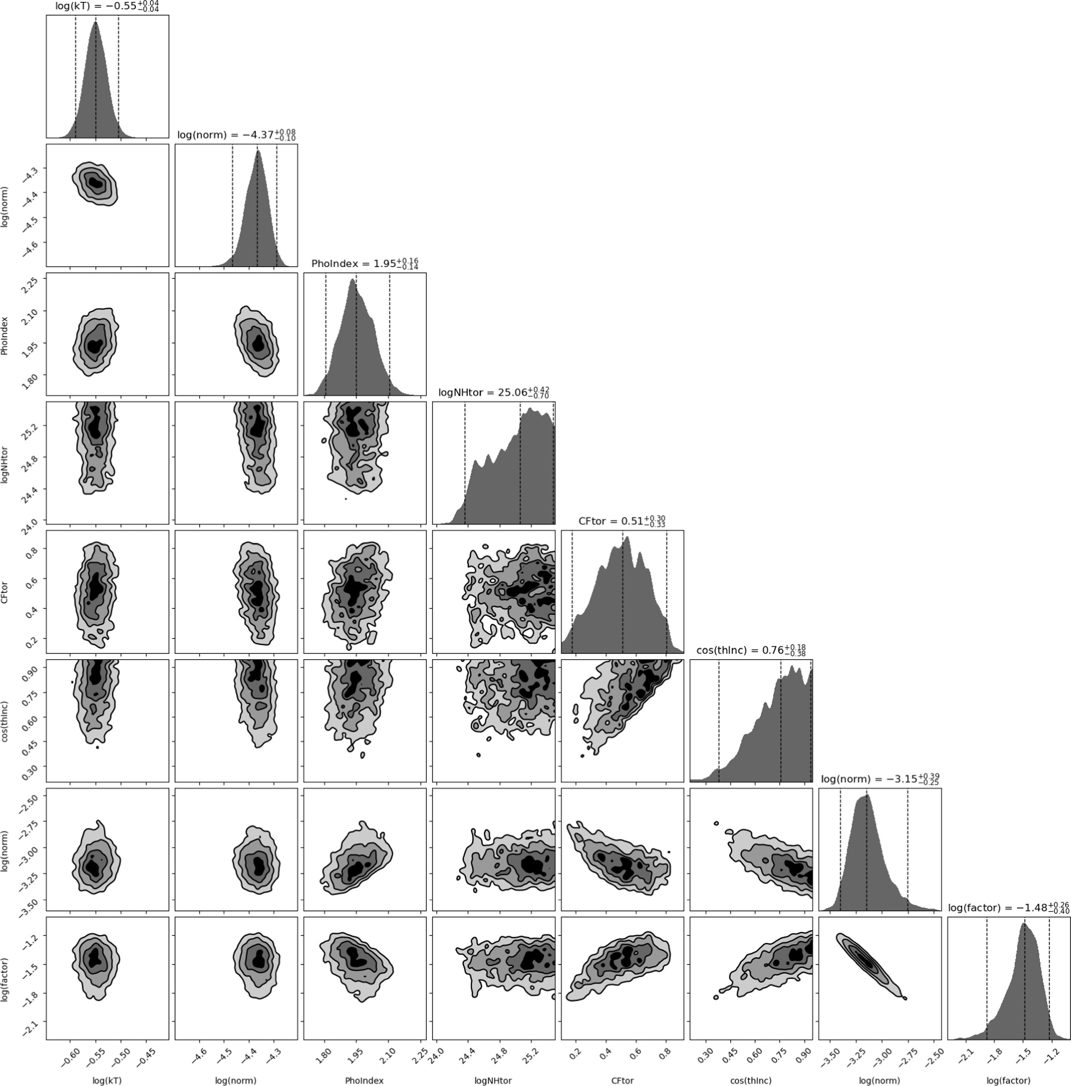
Figure 8. A corner plot showing the posterior probability distributions for the borus02 model in coupled mode. The columns (rows) display the following parameters: (1) logarithm of the apec temperature in kiloelectronvolts; (2) logarithm of the apec normalization; (3) photon index; (4) logarithm of the global column density of the torus; (5) covering factor of the torus; (6) cosine of the inclination angle; (7) logarithm of the power-law normalization; and (8) logarithm of the scattering fraction.
Download figure:
Standard image High-resolution image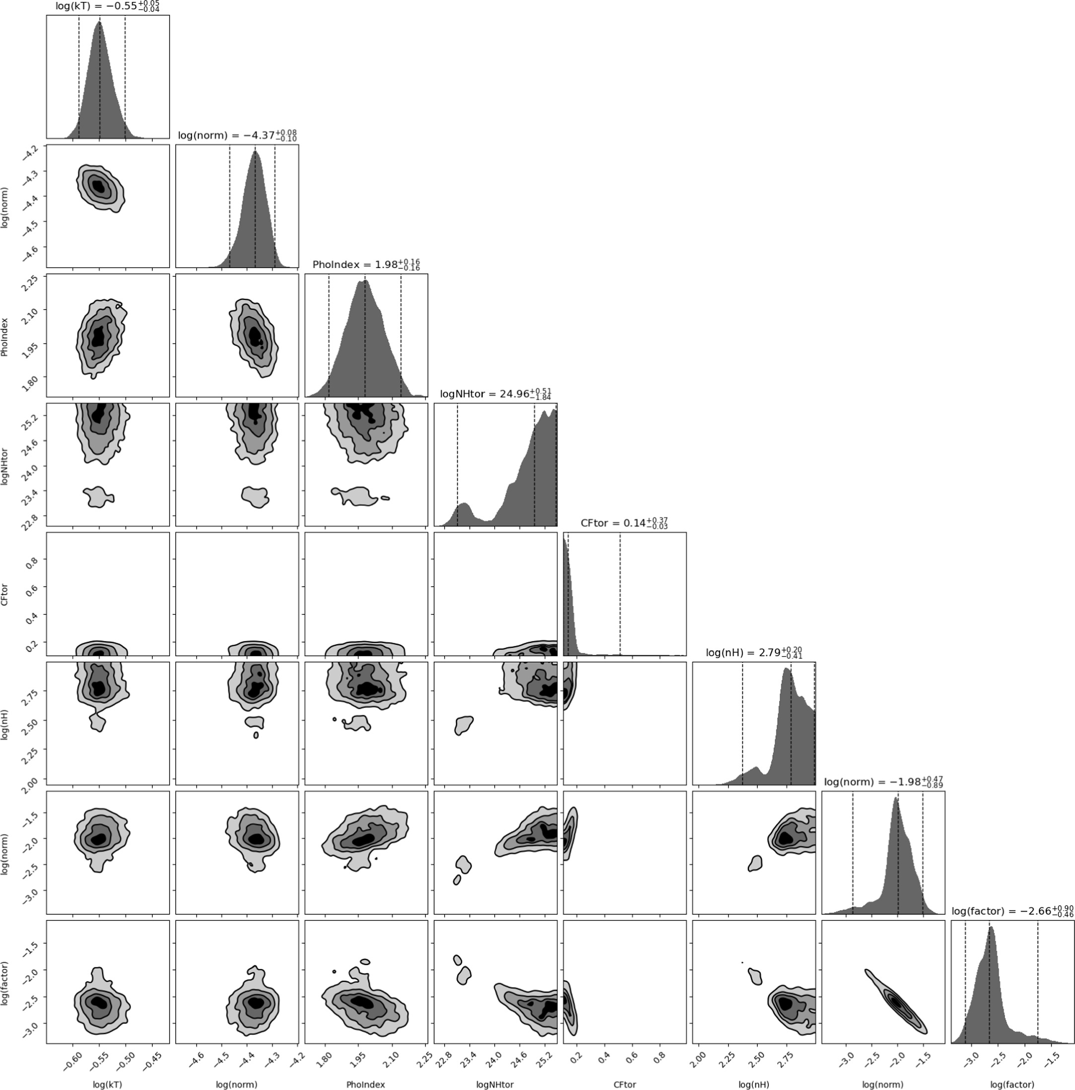
Figure 9. A corner plot showing the posterior probability distributions for the borus02 model in decoupled mode. The columns (rows) display the following parameters: (1) logarithm of the apec temperature in kiloelectronvolts; (2) logarithm of the apec normalization; (3) photon index; (4) logarithm of the global column density of the torus; (5) covering factor of the torus; (6) logarithm of the line-of-sight column density; (7) logarithm of the power-law normalization; and (8) logarithm of the scattering fraction.
Download figure:
Standard image High-resolution image
Figure 10. A corner plot showing the posterior probability distributions for the MYTorus model. The columns (rows) display the following parameters: (1) logarithm of the scattering fraction; (2) logarithm of the apec temperature; (3) logarithm of the apec normalization; (4) photon index; (5) logarithm of the power-law normalization; (6) logarithm of the global column density in units of 1024 cm−2; and (7) cosine of the inclination angle.
Download figure:
Standard image High-resolution image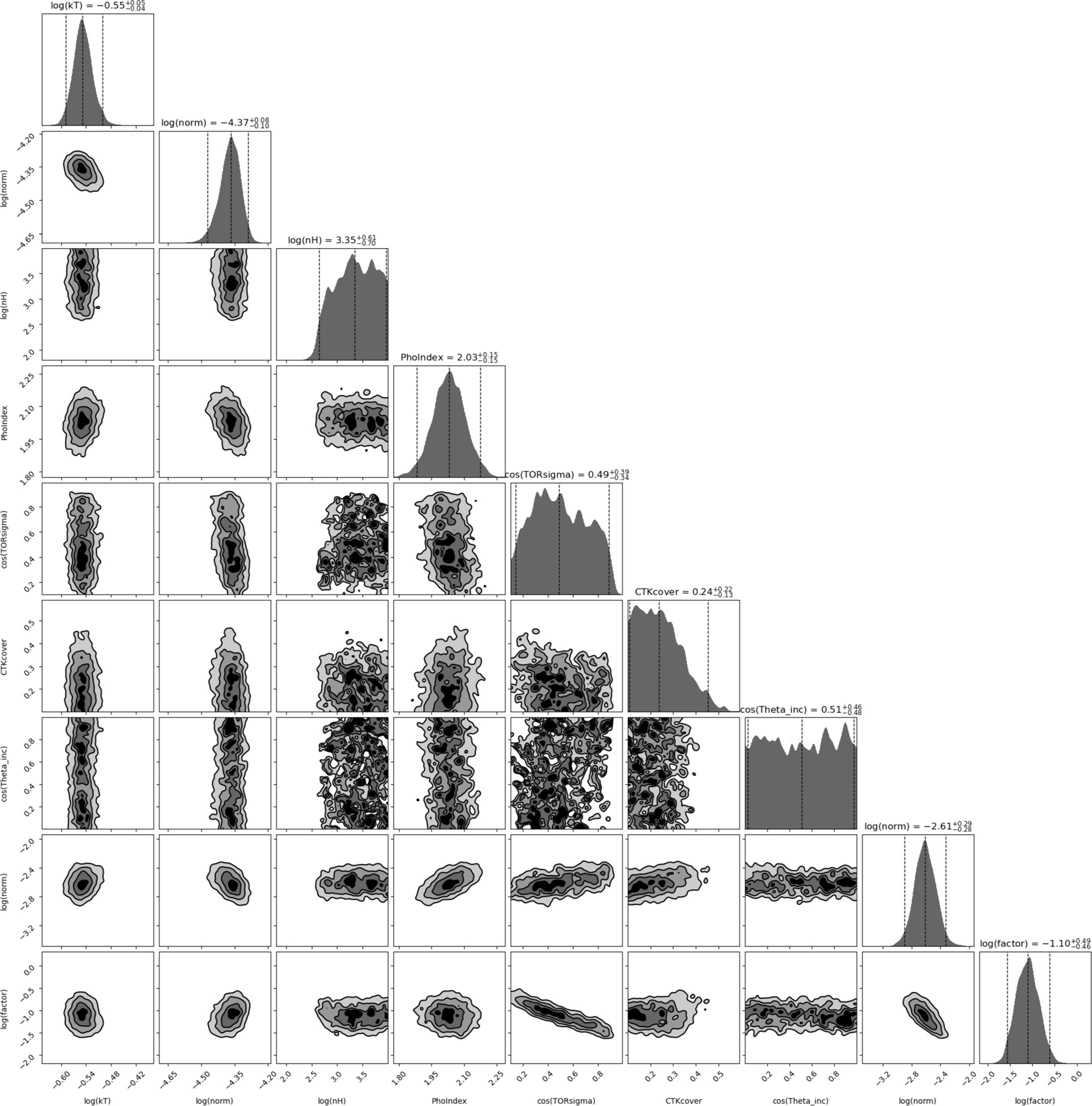
Figure 11. A corner plot showing the posterior probability distributions for the UXCLUMPY model. The columns (rows) display the following parameters: (1) logarithm of the apec temperature; (2) logarithm of the apec normalization; (3) logarithm of the line-of-sight column density in units of 1024 cm−2; (4) photon index; (5) cosine of the torus dispersion TORsigma; (6) Compton-thick inner ring covering factor; (7) cosine of the inclination angle; (8) logarithm of the power-law normalization; and (9) logarithm of the scattering fraction.
Download figure:
Standard image High-resolution image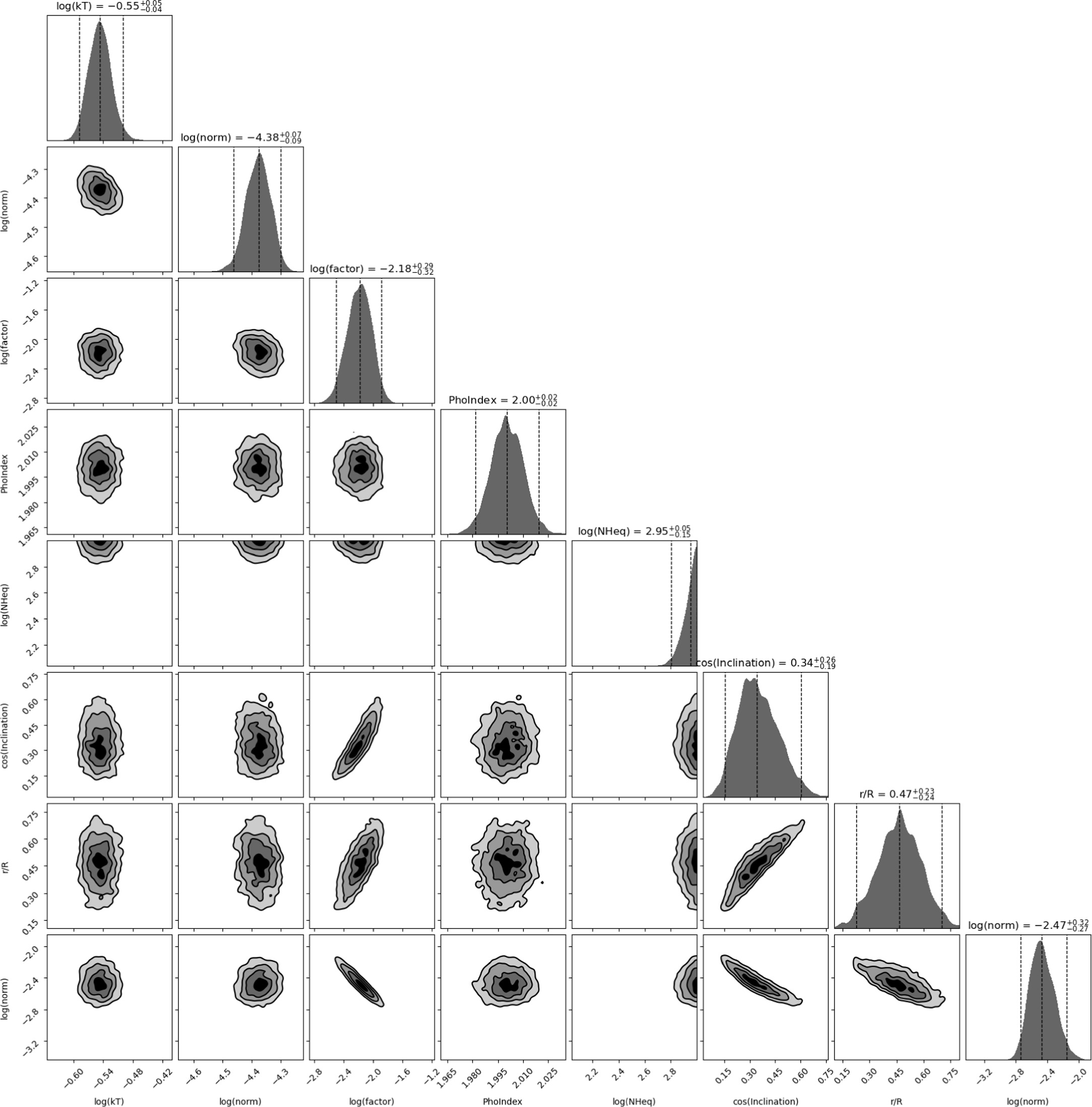
Figure 12. A corner plot showing the posterior probability distributions for the RXTorus model. The columns (rows) display following parameters: (1) logarithm of the apec temperature, (2) logarithm of the apec normalization; (3) logarithm of the scattering fraction; (4) photon index; (5) logarithm of the equatorial column density in units of 1022 cm−2; (6) cosine of the inclination; (7) covering factor given as r/R; and (8) logarithm of the normalization of the power law.
Download figure:
Standard image High-resolution image
Footnotes
- 6
For more information, see: https://heasarc.gsfc.nasa.gov/docs/heasarc/caldb/docs/memos/ogip_92_009/ogip_92_009.pdf.
- 7
- 8
- 9
- 10
- 11
Here we refer to the intrinsic obscurer as the obscurer at the redshift of the source, to distinguish it from the Galactic obscurer. However, no assumption is made to decouple the host galaxy and circumnuclear obscurers in our modeling.
- 12
Available at https://github.com/JohannesBuchner/xars.
- 13
Available at https://www.astro.unige.ch/reflex.
- 14
- 15
We note that the [O iii] and 12 μm luminosities were estimated using different luminosity distances. The maximum difference in the derived 2–10 keV luminosity arising from the discrepant distances does not exceed 0.1 dex.
- 16
We note that with additional scatter, the [O iii] luminosity may be consistent with the results from our analysis.
- 17