Radio Pulsar B0950+08: Radiation in the Magnetosphere and Sparks above the Surface

Zhengli Wang; Jiguang Lu; Jinchen Jiang; Shunshun Cao; Kejia Lee; Enwei Liang; Lunhua Shang; Weiyang Wang; Renxin Xu; Weiwei Zhu

doi:10.3847/1538-4357/ad217a

1. Introduction

The nearby ∼253 ms pulsar PSR B0950+08 has been observed by several groups (e.g., Hankins & Cordes 1981; Hobbs et al. 2004; Johnston et al. 2005; Singal & Vats 2012; Bilous et al. 2022). Hankins & Cordes (1981) pointed out that the separation between the interpulse and main pulse is frequency-independent below 5 GHz and the "low level emission" (the emission from the "bridge" component of the interpulse to the main pulse) of this pulsar is detected over at least 83% of the rotation period, and they argued that these radio emission features could be the result of the magnetic multipole field. Recently, Wang et al. (2022) found that the radio signal of this pulsar is detected over its entire rotation using Five-hundred-meter Aperture Spherical Radio Telescope (FAST) observations. Singal & Vats (2012) presented the detection of its giant pulse emission and showed that the cumulative intensity density distribution of the detectable giant pulses is a power-law function with index −2.2. Bilous et al. (2022) argued that the microsecond-scale fluence variability of single pulses of this pulsar at low frequency may be caused by diffractive scintillation. Everett & Weisberg (2001) proposed an orthogonal rotator for PSR B0950+08 and explained the radiation regions of the main pulse and interpulse as opposite magnetic poles. While the emission mechanism and its location within a pulsar are open questions, polarization studies can help gain insights into them.

After more than half a century since the discovery of pulsars, there is yet no unified understanding of particle creation and acceleration in the magnetosphere (Beskin 2018). The challenges may be the poorly understood physics of the pulsar surface: the vacuum gap model requires strong binding yet the space-charge-limited flow model needs weak binding on the pulsar surface. Inner vacuum accelerators were first proposed and developed by Ruderman & Sutherland (1975, hereafter RS75), with the polar cap radius on the pulsar surface, ${r}_{p}=R\sqrt{R{\rm{\Omega }}/c}\simeq ({10}^{4}\,\mathrm{cm})\,{R}_{6}^{3/2}{P}^{-1/2}$ , for an aligned rotator of radius R = (10⁶ cm) R₆ and angular frequency Ω = 2π/P (c is the light speed). Motivated by explaining both the radio and γ-ray pulse profiles of rotation-powered pulsars and by understanding naturally the global current flows in pulsar magnetospheres, Qiao et al. (2004) proposed an annular gap (AG) model. The open-field-line magnetosphere would then be divided into two regions: the magnetic field lines in an AG region intersect the null charge surface (NCS), while the other region is called a core gap (CG). Certainly, it is not well understood which region dominates the radiation, and a precise analysis of the emission zones of this bright pulsar should provide insight into the pulsar radiation mechanism.

Besides, the emission physics of radio pulsars is closely relevant to the polarization emission properties. First, unraveling the magnetospheric geometries of pulsars depends on the inclination angle between the magnetic and rotation axes. Second, a radio telescope can detect the radiation behaviors of the pulsars such as the average pulse profile, depending on the viewing angle. Finally, the detection of the radiation in the magnetosphere and the mapping of the polar cap sparking also require the study of the polarization behaviors. Therefore, a detailed study of the polarization behaviors provides global knowledge for understanding the radiation mechanism.

We describe the 110 minutes polarization-calibrated data observed with FAST and the data reduction in Section 2. To obtain the polarization emission properties of PSR B0950+08 with radiation over the whole 360° of longitude, we propose two tentative methods of baseline intensity determination in Section 3. The polarization position angle (PPA) is fitted in the classical rotating vector model (RVM, Radhakrishnan & Cooke 1969), and the related results are presented in Section 4. Discussions and conclusions are summarized in Sections 5 and 6, respectively.

2. Observation and Data Reduction

In this work, PSR B0950+08 was observed with tracking mode on MJD 59820 (2022 August 29) using the 19-beam receiver system of FAST (Jiang et al. 2019, 2020). The raw data were recorded in the 8-bit-sampled search mode PSRFITS format (Hotan et al. 2004) with 4096 frequency channels, and the frequency resolution is ∼0.122 MHz. The entire polarization-calibrated observation lasts 110 minutes and the time resolution of the recorded data is 49.152 μs. To obtain the emission properties of single pulses of this pulsar, the DSPSR software package was adopted in the data reduction process (van Straten & Bailes 2011). The option "-s" provided by DSPSR was used to fold the raw data with a resampling time of ∼0.25 ms. In order to obtain accurate polarization calibration solutions, the polarization calibration signals of 30 s were injected after each subintegration for 30 minutes. Besides, the radio frequency interference is eliminated using the frequency–time dynamics spectrum.

3. Baseline Intensity Determination

Conventional baseline subtraction is used to subtract the weak emission region from the strong emission region (i.e., the main pulse) of the pulsar, but it would not be suitable for PSR B0950+08 since the radio signal of this pulsar is detected over the whole pulse phase (Wang et al. 2022). To detect the baseline intensity of this pulsar, two tentative determinations of it are proposed.

PSR B0950+08 is a bright pulsar located nearby, with a dispersion measure (DM) of 2.97 pc cm⁻³, which indicates that the average pulse profile of this pulsar is little affected by the effect of interstellar scintillation. Previous observations of PSR B0950+08 have not detected any mode-switching behavior (e.g., Hankins & Cordes 1981; Singal & Vats 2012; Bilous et al. 2022; Wang et al. 2022), so its average pulse profile is stable at a narrow observing frequency. In addition, the stable profile is related to the integration, and the average pulse profiles of radio pulsars are quite stable over long integration. In this work, the emission property whereby the average pulse profile of this pulsar is stable over long integration is used to detect its baseline. To obtain the stable profile of the subintegration of this pulsar, the 110 minutes polarization-calibrated observation is segmented into two subintegrations of 55 minutes. Considering the relationship between the average pulse profiles of the two subintegrations of this pulsar and its baseline intensity, we could have

$\begin{eqnarray}&&{I}_{e1}-{I}_{b}=\kappa ({I}_{e2}-{I}_{b}),\end{eqnarray} \tag{ 1 }$

where κ is a parameter that reflects the fluctuations in the radio emission intensity of this pulsar over different subintegrations, and it would be equal to 1 for infinite integration. Here, I_e1 and I_e2 denote the average radio intensity of this pulsar over its entire 360° of longitude for the first and second subintegrations, respectively. I_b corresponds to the baseline intensity of the entire 110 minutes observation. A detailed derivation of Equation (1) is presented in the Appendix. The result of subtracting PSR B0950+08's baseline intensity according to Equation (1) is shown in the left-hand panels of Figure 1.

**Figure 1.** The RVM fit for the pulse longitudes whose linear fractions are higher than ∼30% of the whole pulse phase of the radiative pulsar PSR B0950+08. The left-hand panels show the total emission intensity (black curve) and the linear fraction (red curve). The observed PPAs and best RVM fit (red line) are shown in the middle panel, and indicate that the inclination angle α and the impact angle β (β = ζ − α) are 1005 and −332, respectively. The errors between the RVM fit curve and observed PPAs are plotted in the bottom panel, and those values that fall in the range from −5° to 5° are believed to be the RVM intervals. Two vertical gray regions are unweighted in the fit because the one on the left indicates the bridge component, whose polarization emission property is detected with large uncertainty. The right-hand gray region is the main pulse region, whose polarization emission displays depolarization and jumps in position angle, and these complex polarization emission phenomena are not described by the RVM. I and M indicate the locations of the peaks of the interpulse and the main pulse in the top panel, respectively. The steepest gradient of the RVM fit curve has been centered. The right-hand panel shows the α–ζ plane, which depicts the value of ${\chi }_{\mathrm{reduced}}^{2}$ from the fitting routine, and the black cross denotes the location of the minimum of the ${\chi }_{\mathrm{reduced}}^{2}$ surface. We select also two other parameter sets of {α, β}: two crosses (magenta and green) in the right panel and their corresponding RVM curves (magenta dotted and green dashed curves) in the left panel, indicating that the differences between the three groups of RVM solutions are minimal.
Download figure:
Standard image High-resolution image

fdg — **Figure 1.** The RVM fit for the pulse longitudes whose linear fractions are higher than ∼30% of the whole pulse phase of the radiative pulsar PSR B0950+08. The left-hand panels show the total emission intensity (black curve) and the linear fraction (red curve). The observed PPAs and best RVM fit (red line) are shown in the middle panel, and indicate that the inclination angle α and the impact angle β (β = ζ − α) are 1005 and −332, respectively. The errors between the RVM fit curve and observed PPAs are plotted in the bottom panel, and those values that fall in the range from −5° to 5° are believed to be the RVM intervals. Two vertical gray regions are unweighted in the fit because the one on the left indicates the bridge component, whose polarization emission property is detected with large uncertainty. The right-hand gray region is the main pulse region, whose polarization emission displays depolarization and jumps in position angle, and these complex polarization emission phenomena are not described by the RVM. I and M indicate the locations of the peaks of the interpulse and the main pulse in the top panel, respectively. The steepest gradient of the RVM fit curve has been centered. The right-hand panel shows the α–ζ plane, which depicts the value of ${\chi }_{\mathrm{reduced}}^{2}$ from the fitting routine, and the black cross denotes the location of the minimum of the ${\chi }_{\mathrm{reduced}}^{2}$ surface. We select also two other parameter sets of {α, β}: two crosses (magenta and green) in the right panel and their corresponding RVM curves (magenta dotted and green dashed curves) in the left panel, indicating that the differences between the three groups of RVM solutions are minimal.
Download figure:
Standard image High-resolution image

On the other hand, a model based on the polar cap's electric field distribution properties is put forward here to help subtract the baseline. We assume that the polar cap of a pulsar is a voltage-regular diode. The spark discharge can be considered as the breakdown of the voltage-regular diode, whose breakdown voltage is assumed as V₀. Consequently, the distribution of the voltage of the base and top edges of the voltage-regular diode can be regarded as $V\sim { \mathcal N }({V}_{0},{\sigma }_{V}^{2})$ . Here V and σ_V denote the voltage of the two edges of the voltage-regular diode and its standard deviation. According to the property of the Gaussian white noise distribution, the fluctuation voltage distribution of the two edges of the voltage-regular diode caused by each spark discharge is set to ΔV, which follows ${ \mathcal N }(0,2{\sigma }_{V}^{2})$ . Compared with V₀, ΔV is a small variation (i.e., ΔV ≪ V₀). Therefore, the energy of each polar cap spark discharge can be estimated, and its distribution is ${ \mathcal N }(0,4{V}_{0}^{2}{\sigma }_{V}^{2})$ .

Considering that the spark discharge is equivalent to converting the electric field energy of a pulsar into the number of electrons N, the accelerating electric field (which corresponds to the component of the electric field in the pulsar magnetosphere parallel to the magnetic field) of a pulsar is hardly changed. Therefore, the energy of the accelerated electrons is thought to be a constant. Furthermore, the radiative spectrum of a group of electrons is also hardly changed. Nonetheless, its flux has a significant change since it depends on the number density of the electrons n_e. The number of electrons produced by the spark discharge can be regarded as the number density of the electrons because the electrons escape from the polar cap of a pulsar at almost the same time. Considering that the radiation of a pulsar is coherent, the radiation energy is proportional to N². Consequently, the radiation energy released by each spark discharge is equal to the square of the Gaussian distribution. In the radiation of radio pulsars, each emission phase point may include multiple spark discharge processes, so the flux distribution of this emission phase point can be estimated, and it is equal to the sum of squares of multiple Gaussian distributions (i.e., a χ² distribution). We assume that the distribution of the total number of spark discharge processes follows the Poisson distribution in the polar cap of a pulsar.

Considering the properties of the χ² distribution and the Poisson distribution, the relationship between the radio emission of this pulsar and its baseline intensity can be given as

$\begin{eqnarray}&&{({I}_{e}-{I}_{b})({D}_{e}-{D}_{b})=\kappa ({S}_{e}-{S}_{b})}^{2}\end{eqnarray} \tag{ 2 }$

where I_e, S_e, and D_e denote the radio emission intensity, variance, and central moment of the third order of this pulsar, respectively. The intensity, variance, and central moment of the third order of the baseline of this pulsar are denoted as I_b, S_b, and D_b, respectively. Here κ is a parameter that reflects the fluctuations in the radio emission intensity of this pulsar over different subintegrations. The result is consistent with Equation (1).

Meanwhile, conventional baseline subtraction is also taken into account. Considering the radio emission properties of PSR B0950+08 (Wang et al. 2022), the bridge component between the main pulse and interpulse accounts for ∼5% of the rotation period of this pulsar and is regarded as its baseline intensity. The result is shown in Figure 2. The legends and indications are the same as in Figure 1, but for taking the bridge component between the two vertical blue lines as the reference of the baseline. In comparison to the left-hand panel of Figure 1, there are noticeable differences in the PA-swings of the weak emission regions, such as the precursor component of the main pulse and the postcursor component of the interpulse. Further discussion of these differences will be presented in later sections.

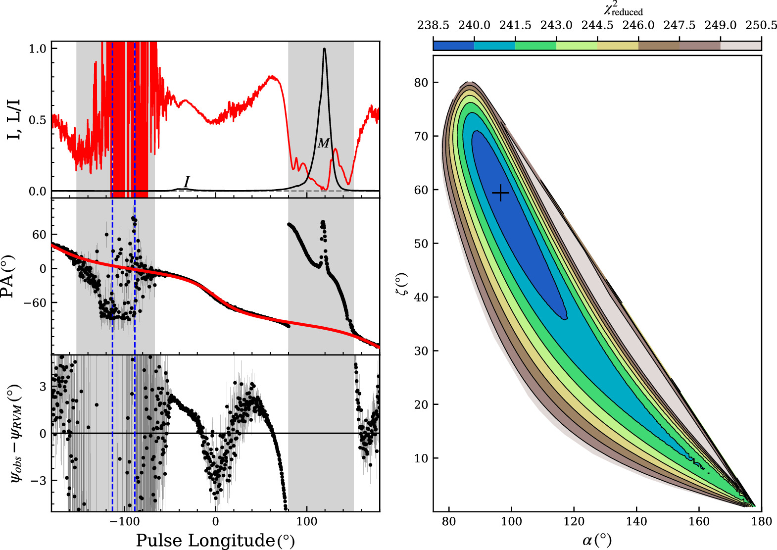
**Figure 2.** Same as Figure 1, but the region between the two vertical dashed blue lines is regarded as the reference of the baseline. The right-hand panel indicates that the inclination angle α = 965 and the impact angle β = −371 (β = ζ − α). It should be noticed that the values of ${\chi }_{\mathrm{reduced}}^{2}$ are about ten times as large as the values of ${\chi }_{\mathrm{reduced}}^{2}$ given in the right-hand panel of Figure 1.
Download figure:
Standard image High-resolution image

fdg — **Figure 2.** Same as Figure 1, but the region between the two vertical dashed blue lines is regarded as the reference of the baseline. The right-hand panel indicates that the inclination angle α = 965 and the impact angle β = −371 (β = ζ − α). It should be noticed that the values of ${\chi }_{\mathrm{reduced}}^{2}$ are about ten times as large as the values of ${\chi }_{\mathrm{reduced}}^{2}$ given in the right-hand panel of Figure 1.
Download figure:
Standard image High-resolution image

4. Results

4.1. Polarization Emission Property

Two tentative baseline intensity determinations for PSR B0950+08 described in Section 3 are proposed, and the conventional baseline subtraction is also taken into account. After subtracting the baseline of this pulsar using three methods, the polarization emission properties of the main pulse and interpulse are consistent, but the PA-swings of the weak emission region (i.e., the precursor of the main pulse and the postcursor of the interpulse) have little difference.

The polarization emission properties of this pulsar are shown in the left-hand panels of Figures 1 and 2. It can be found that the polarization emission of the main pulse displays a depolarization phenomenon (the linear fractions are less than ∼10%), and there is a significant jump in position angle at the location of the peak of the main pulse. Detailed discussions of the physical mechanism of the depolarization and jumps in position angle of radio pulsars are presented in Xu et al. (1997), and they concluded that these polarization emission behaviors may be caused by a phase shift of the beam centers of the different components of the pulsars. Other possible origins of the jump such as the orthogonal polarization modes (OPMs) also discussed in detail (e.g., Dyks 2017). Moreover, the curve of the linear fraction of the main pulse becomes complicated, and the values jump at some pulse longitudes. To reveal the polarization emission properties of this pulsar, the baseline position is also indicated by the gray dashed line in the top panels.

4.2. Fitting Polarization Position Angle with RVM

To understand the magnetospheric geometry of PSR B0950+08, the classical RVM is used to fit the observed PPAs of this pulsar (Radhakrishnan & Cooke 1969). The PPAs of the pulse longitudes whose linear fractions are higher than ∼30% are considered in the fit, and further discussion will be summarized in Section 5. After taking the position of the steepest gradient of the RVM fit curve as the reference pulse longitude 0°, the results are shown in Figure 1. It can be found that the steepest gradient of the RVM fit curve (at the reference pulse longitude 0°) approaches the interpulse. This property demonstrates that the magnetic pole is closer to the interpulse than to the main pulse.

In the α–ζ panel, the values of ${\chi }_{\mathrm{reduced}}^{2}$ are indicated by the colors. The black cross denotes the minimum value of ${\chi }_{\mathrm{reduced}}^{2}$ in the fit, and it gives the values of the viewing angle ζ = 67 fdg 3 and the inclination angle α = 100 fdg 5. Compared with this result, the baseline of this pulsar is subtracted using the conventional method, and the results are shown in Figure 2. The right-hand panel indicates the viewing angle ζ = 59 fdg 4 and the inclination angle α = 96 fdg 5. The region between the two vertical blue lines is believed to be the baseline region since it is far away from the main pulse. Compared with other pulse longitudes, the impulsive radio emission detected in the chosen region is extremely weak and close to the baseline intensity. This region is regarded as the reference of the baseline, and subtracting it minimizes the effect of baseline subtraction on the pulsar with emission features of the whole 360° of longitude (Wang et al. 2022). One can see that the values of ${\chi }_{\mathrm{reduced}}^{2}$ of this RVM solution of α and ζ are about ten times as large as the values of ${\chi }_{\mathrm{reduced}}^{2}$ of the results shown in the right-hand panel of Figure 1, and the distribution of α and ζ of this RVM solution is wider, which means a larger uncertainty. For these reasons, α = 100 fdg 5 and ζ = 67 fdg 3 are used for the later analyses of this work. The RVM solutions of α and ζ given in Figures 1 and 2 are consistent with each other.

4.3. The Radiative Geometry in the Magnetosphere

The magnetospheric geometry of PSR B0950+08 is revealed by assuming the magnetic dipole field. Figure 3(a) depicts the three-dimensional magnetospheric geometry of this pulsar. Figure 3(b) describes the magnetospheric geometry of this pulsar in the Ω– μ plane, and the light cylinder radius of this pulsar is represented by the vertical dotted lines. Its rotation axis is upward, and the magnetic axis is inclined at an angle α in the Ω– μ plane. The null charged surface is the surface where the magnetic field line is perpendicular to the rotation axis (i.e., Ω · B = 0) and it is indicated by the red dotted lines (labeled NCS). Detailed descriptions of these figures are given in their captions.

fdg — **Figure 3.** The radiation geometry of PSR B0950+08 using the RVM solutions of α = 1005 and β = −332. (a) Three-dimensional magnetospheric geometry of the magnetic dipole field of this pulsar. To understand the magnetospheric geometry, the magnetic pole whose angle with respect to the rotation axis is α = 1005 is defined as the magnetic Pole 1 in the Ω– μ plane. Its opposite magnetic pole is defined as the magnetic Pole 2. The last closed field lines are indicated by the cyan curves, and the magnetic field lines originating from the polar cap of magnetic Pole 1 and Pole 2 are denoted by blue and red curves, respectively. In addition, the line of sight (LOS) is indicated by the dashed arrow. (b) The magnetospheric dipole geometry of this pulsar in the Ω– μ plane. The light cylinder radius is indicated by the vertical dotted lines. The line of sight (red arrow) and the null charged surface (NCS, red dashed line) are also shown. To reveal the width of the annular gap (AG) and the core gap (CG), the areas between the critical field lines and the last closed field lines depicting the AG are filled in gray, and the CG describing the zones between the magnetic axis and the critical field lines is filled in yellow in the right-hand diagram. The cyan lines depict the magnetic field lines that only cross the light cylinder on the side of the opposite magnetic pole. The magnetic field lines inside and outside the corotating frame of this pulsar are indicated by solid and dotted lines, respectively. In panel (b), to display clearly the global magnetosphere as well as the polar cap's surroundings, the ratio of the vertical to horizontal dimensions is chosen as 3:1 for the left-hand diagram, but 4:3 for the right-hand one.
Download figure:
Standard image High-resolution image

To understand the γ-ray and radio emission from the pulsar, Qiao et al. (2004) proposed a new segment of the polar cap of the pulsar (Ruderman & Sutherland 1975). The conventional RS75-type gap model is segmented into the AG and CG, and the boundary between them is defined by the magnetic field lines intersecting the NCS. The AG describes the region between the last closed field lines and the critical field lines (the magnetic field lines are perpendicular to the rotation axis (i.e., Ω · B = 0) at the light cylinder); the CG is surrounded by the critical field lines.

The AG and CG are also plotted in the right-hand panel of Figure 3. To show the width of the two gaps, the AG and CG are filled in gray and yellow colors, respectively. In the polar cap between the magnetic and rotation axes, the CG is extremely narrow compared to the AG. Moreover, the width of the CG is also less than the width between the equator and the magnetic axis since the equator falls in the gray regions in the magnetic Pole 1. One can see that the last closed field lines become more elliptical. For the pulsar whose inclination angle is α < 90°, as pointed out by Qiao et al. (2004), the width of the AG between the magnetic axis and the equator becomes greater when α increases. In contrast, the AG between the magnetic and rotation axes becomes narrower. The width of the AG of PSR B0950+08 is different in scenarios with α < 90° (Qiao et al. 2004). Figure 3(b) shows, the equator falls in the region between the magnetic and rotation axes. The AG between the magnetic axis and equator (or rotation axis) becomes wider, but the AG between the magnetic axis and the direction antiparallel to the rotation axis becomes narrower. In magnetic Pole 2, the variation of the width of the AG is similar to the scenarios for α < 90° discussed in Qiao et al. (2004).

In the AG and CG models, the potential drop of the polar cap of the pulsar is related to the width of the AG. A wider AG results in a greater potential drop, making it easier to produce sparks. Based on this physical picture, in magnetic Pole 1, it is easier to produce sparks in the opening field line region between the magnetic and rotation axes than in the region between the magnetic axis and the direction antiparallel to the rotation axis. In contrast, it in magnetic Pole 2, is easier to produce sparks in the region between the magnetic axis and the equator than in the opening field line region between the magnetic and rotation axes.

It can be seen that the magnetospheric structure of this pulsar becomes complex if the inclination angle α is large. As Figure 3(b) shows, the cyan field lines only cross the light cylinder on the side of the opposite magnetic pole. This structure implies that in some of the opening field line regions the magnetic field lines do not pass through the light cylinder.

4.4. Emission Zones in Both Regions of AG and CG

We unravel the polar cap surface of PSR B0950+08 based on the 110 minutes polarization observation under the framework of the dipole field. To understand which opening field line region dominates this pulsar's radiation, the AG and CG of the vacuum gap model are used to reveal its emission geometry. The shapes of the AG and CG of the dipole field of PSR B0950+08 at the stellar surface are shown in Figures 4 and 5, and two-pole model scenarios are plotted. A detailed description of the emission zone is given in the caption of the figure.

**Figure 4.** Polar cap shape of PSR B0950+08: the AG and CG of this pulsar are plotted. The black (red) lines represent the intersection curve of the stellar surface and the last closed field lines (the critical field lines). The black dot (x mark) indicates the magnetic pole in the left (right) panel. As shown in the figure, the AG describes the zones between the black and the red curves, and the CG is surrounded by the red curve. The radiation of the AG is first used to explain the radio emission of this pulsar. Without loss of generality, we assume that the radio emission of this pulsar comes from these magnetic field lines whose footprints are concentrated on the orange line. To unveil the radiation trajectories, the radiation phase is calculated, and its values are indicated by the colors. The dot denotes the location of the peak of the interpulse (labeled I) in the left panel, and it represents the location of the peak of the main pulse (labeled M) in the right panel. The magnetic field lines whose footprints are concentrated on the orange curve are indicated by the solid line, while their radiation directions are parallel to the line of sight inside the corotating frame of this pulsar. The footprints of the magnetic field lines whose radiation directions are not parallel to the line of sight are denoted by the dashed line. To unravel the emission geometry of this pulsar even further, the PPAs are also plotted (gray dashed lines). Θ and Φ denote the polar and azimuthal angles around the magnetic axis, respectively.
Download figure:
Standard image High-resolution image

**Figure 5.** Same as Figure 4 except for assuming that the radio emission of this pulsar originates from the CG.
Download figure:
Standard image High-resolution image

One can see that the equator of this pulsar falls in the region between magnetic and rotation axes; this structure differs from scenarios with α < 90° discussed in Qiao et al. (2004). Qiao et al. (2004) considered the magnetospheric geometry of the magnetic dipole field of the pulsars for different inclination angles α (i.e., α = 0°, 45°, 75°), and they found that the width of the AG is a function of the inclination angle α. The left-hand panel of Figure 4 shows that the width of the AG between the magnetic and rotation axes is greater than that between the magnetic axis and the antiparallel direction of the rotation axis. In contrast, from the right-hand panel, the variation of the width of the AG is similar to that in Qiao et al. (2004) since the value of the inclination angle is α = 79 fdg 5 in the magnetic Pole 2. As Figure 3(b) shows, the AG between the magnetic axis and the antiparallel direction of the rotation axis becomes narrow, because the critical field lines that fall in the region between the magnetic axis and the cyan magnetic field lines are perpendicular to the rotation axis (i.e., Ω · B = 0) only when they intersect with the light cylinder on the opposite side in the Ω– μ plane.

4.5. A Two-pole Model of PSR B0950+08

Charged particles will emit radiation as they move along the magnetic field lines whose intersection curves with the stellar surface are inside the polar cap of the pulsar (e.g., Ruderman & Sutherland 1975; Arons & Scharlemann 1979). The radiation of the charged particles will be detected by the telescope when it is directed parallel to the line of sight. The magnetic field lines in the corotating frame of the pulsar have no more than one point where the radiation direction is parallel to the line of sight before they intersect with the light cylinder. Therefore, the radiation phase of the emission points whose radiation directions are parallel to the direction of the line of sight can be determined.

Both the AG and the CG are taken into account to understand the radio emission features from PSR B0950+08. As Figure 4 shows, without loss of generality, the orange curve obtained by averaging the distances between the last closed field lines (black curve) and the critical field lines (red curve) is used to denote the radiation generated from the AG. According to the result of the calculations, the radio emission of this pulsar originates from the magnetic Pole 1 shown in the left-hand panel, and the radiation generated from its opposite magnetic pole is described in the right-hand panel. When the radiation direction of the magnetic field lines is parallel to the line of sight, the magnetic field lines whose footprints are concentrated on the orange curve are indicated by the solid line. Meanwhile, the CG scenario is shown in Figure 5, where the two-thirds distances between the critical field lines (red curve) and the magnetic pole are used to indicate the radiation of the CG.

According to the radio emission properties of PSR B0950+08 (Wang et al. 2022) and its magnetospheric geometry based on the polarization-calibrated observation in this work, the emission points whose radiation directions are parallel to the line of sight can be determined using the geometric relation $\zeta ={\cos }^{-1}({\hat{{\boldsymbol{B}}}}_{{\boldsymbol{z}}}/\sqrt{{\hat{{\boldsymbol{B}}}}_{{\boldsymbol{x}}}^{2}+{\hat{{\boldsymbol{B}}}}_{{\boldsymbol{y}}}^{2}+{\hat{{\boldsymbol{B}}}}_{{\boldsymbol{z}}}^{2}})$ , where $\hat{{\boldsymbol{B}}}={\hat{{\boldsymbol{B}}}}_{{\boldsymbol{x}}}+{\hat{{\boldsymbol{B}}}}_{{\boldsymbol{y}}}+{\hat{{\boldsymbol{B}}}}_{{\boldsymbol{z}}}$ is the unit vector of the magnetic field of the emission point. To exhibit the radiation trajectories of this pulsar, the radiation phase is calculated, and its values are indicated by the colors. After taking the steepest gradient of the RVM fit curve as the reference pulse longitude 0°, Figure 1 indicates that the locations of the peak of the interpulse and main pulse are −25° and 125°, respectively. The locations of the peak of the interpulse and main pulse are also noted in Figure 4. One can see that the radio emission of the pulse longitudes from ∼−85° to ∼85° of this pulsar originates from the magnetic Pole 1, while the radio emission of the remaining 52% of the rotation period comes from its opposite magnetic Pole 2. As Figure 1 shows, the polarization emission properties of this pulsar originating from the magnetic Pole 1 can be described well by the RVM curve. Meanwhile, the radio emission of the main pulse comes from the opposite magnetic Pole 2. The polarization emission properties of the main pulse display depolarization and a jump in position angle. These polarization phenomena imply that the polarization emission originating from the magnetic Pole 2 deviates significantly from the RVM.

Figure 5 shows that the radiation is generated from the CG. Similar to the radiation of the AG scenario, we assume that the magnetic field lines whose footprints are concentrated on the orange curve indicate the radiation of the CG. It can be seen that the radiation of the pulse longitudes from ∼−75° to ∼75° originates from the magnetic Pole 1, and the radiation of the remaining 58% of the rotation period of PSR B0950+08 comes from the magnetic Pole 2.

The phenomenological model used to explain the radio emission properties of PSR B0950+08 can provide further insight into the emission zone, but for the actual scenario, the magnetic field lines intersecting with the stellar surface would become more complex. Considering the radiation characteristics of the whole pulse phase and the polarization emission features, the calculations of the radiation of the AG and the CG models indicate that the emission in the interpulse comes from the magnetic Pole 1, while the radiation of the main pulse originates from the magnetic Pole 2.

4.6. The Emission Height

Based on the result of the mapping sparks on the polar cap surface shown in Figures 4 and 5, the emission height can be calculated according to the three-dimensional calculations of the pulsar emission height given in Zhang et al. (2007). With the AG model, the height of the emission point can be calculated. The results are shown in Figure 6, and the emission heights are indicated by the colors. The left-hand panel shows the emission height of the magnetic Pole 1, and the altitudes range from ∼3000 to ∼7000 km. The emission heights of the radiation phase that originates from the magnetic Pole 2 are shown in the right-hand panel, which indicates that they range from ∼3200 to ∼7800 km. It can be seen that the emission heights of the interpulse and main pulse are ∼3500 km and ∼5000 km, respectively. Moreover, the bridge component is emitted from a higher altitude of approximately 7800 km. One can find that the variation in the emission height is related to the distance between the emission regions and the magnetic pole. The calculation indicates that the emission height of the region that approaches the magnetic pole changes slowly. Meanwhile, the emission height changes sharply when the emission zone is distant from the magnetic pole.

**Figure 6.** The emission height of this pulsar for the AG model. The left-hand panel indicates the emission heights of the magnetic Pole 1, and the interpulse comes from ∼3500 km. The altitudes of the magnetic Pole 2 are plotted in the right-hand panel, which shows that the emission height of the main pulse is ∼5000 km. One can see that the emission height of the main pulse is greater than that of the interpulse. The bridge component originates from an extremely high altitude of ∼7800 km. The light cylinder radius of this pulsar is R_LC ∼ 12,000 km. To further clarify the emission geometry of this pulsar, the PPAs are also included in the plots (gray dashed lines).
Download figure:
Standard image High-resolution image

With the CG scenario, the emission height is also calculated, and the results are shown in Figure 7. One can see that the variation of the emission height is similar to the AG scenario, but the emission heights of the CG are generally higher than those of the AG. Furthermore, it can be found that the emission height of the bridge component even reaches ∼8500 km.

The analysis of the AG and the CG models indicates that PSR B0950+08 is a high-altitude magnetospheric emission pulsar. High radiation altitudes challenge the conventional particle acceleration mechanism and coherent emission mechanism of radio pulsars (Ruderman & Sutherland 1975). With the high radiation altitudes and the radiation characteristics of the whole pulse phase, PSR B0950+08 may have an additional accelerating electric field such as the slot gap accelerator (Arons 1983) or annular gap accelerator (Qiao et al. 2007) to accelerate the charged particles.

5. Discussions

The pulsar's surface physics is hard to probe due to the absence of direct observations. Compared with other normal radio pulsars, the emission geometry of PSR B0950+08 would be good for unraveling the electrodynamics of the pulsar magnetosphere related to the stellar surface. Recently, several research groups have published polarimetric emission characteristics of radio pulsars. Johnston et al. (2023) reported the application of the RVM to a sample of 854 radio pulsars observed with the MeerKAT telescope. They argued that the average PPA tracks of 60% of the pulsars can be described by the RVM. For the pulsars with good RVM fits, their polarization emission features are similar to the Vela pulsar with a high fraction of linear polarization. Rankin et al. (2023) presented the polarization emission properties for 60 radio pulsars using the Arecibo radio telescope. They did not present the RVM fits for these objects, but the variation of the PPAs of these pulsars can be revealed by analyzing their Stokes parameter profiles. It can be found that the polarization behaviors of the pulsars with visible linear polarization fractions in the emission regions are also similar to that of the Vela pulsar. Moreover, Wang et al. (2023) published the polarization profiles of 682 pulsars using the FAST radio telescope. For the pulsars with a high fraction of linear polarization, the steepest gradients of the RVM-fitted curves are almost aligned with the radio emission peaks, implying that the sparking on the polar cap surface for these pulsars is regular and symmetrical.

The emission geometry of PSR B0950+08 could be applied to understand the radiation in the magnetosphere and the sparking on the polar cap surface for normal radio pulsars whose emission occupies almost the whole pulse phase (e.g., PSRs J1851+0418, J1903+0925, J1916+0748, and J1932+1059; e.g., Wang et al. 2023). In the future, we will continue to investigate the emission geometries of the four normal pulsars with extremely wide profiles using the FAST radio telescope. The number of pulsars that exhibit radio emission peaks misaligned with their magnetic poles after accurately mapping the sparks on the polar cap surfaces and whether these pulsars occupy a specific region in the $P\mbox{--}\dot{P}$ diagram are questions that need to be studied further. It is worth investigating whether the emission geometries of these objects with extremely wide profiles can better reflect the physics of their polar cap surfaces. The FAST radio telescope will play a key role in unraveling the stellar surface and even in understanding the radiation mechanism of the radio pulsar, which is our interest now.

Up to now, the offsets of the point of highest PA slope with respect to the radio emission peak are small compared to that of PSR B0950+08 (e.g., Johnston et al. 2023; Wang et al. 2023). The offset for PSR B0950+08 is approximately equal to 60° in the framework of the two-pole model. Most radio pulsars have offsets less than 25°, and those of a few pulsars reach 45°. Small offsets are understandable, explained by the underlying physics of rotation-induced relativistic effects (i.e., aberration and retardation), which do not reflect the electrodynamics of the magnetosphere related to stellar surface physics. The maximum offset between the point of the highest PA slope and the radio emission peak is found based on the 110 minutes polarization observation with the FAST radio telescope. After mapping the sparking points on the surface (see Figures 4 and 5), the polar cap sparking pattern of PSR B0950+08 implies that the distribution of sparks is asymmetrical and irregular. This finding can bring new ideas into the pulsar's surface physics and even its inner dense matter. A pulsar's magnetospheric plasma and its inner dense matter are separated by the stellar surface, and the radiative mechanism could thus be essentially a problem relevant to the nature of the pulsar's surface and even of cold matter at supranuclear density. This relationship could be revealed by the polarization observation of PSR B0950+08: being Gaussian-like means that pulse profiles would usually peak at the maximum slopes of PPA sweep (e.g., the Vela pulsar; Radhakrishnan & Cooke 1969); however, both the main pulse and interpulse from two poles are not at the maximum of PSR B0950+08. Vela-like polarization could be understandable if sparking points are distributed regularly along either AG or CG trajectories on the polar cap and the consequent pair-plasma moves along a flux tube,¹⁰ forming a fan-shaped pattern (Wang et al. 2014). However, as illustrated in Figures 5–8, the mapped sparks on PSR B0950+08's surface are inhomogeneously distributed away from the magnetic pole. This may hint at preferential discharges somewhere on the polar cap due to a rough pulsar surface (there are protuberances, or small mountains, on the stellar surface that would make its surface rough), as had already been proposed for understanding FAST's single pulse observation of PSR B2016+28 (Lu et al. 2019). Regular drifting sparks are speculated to occur for Vela-like young and energetic pulsars, while sparse sparks are for old and lazy ones whose magnetospheric activity is weak.

In what kind of model of a pulsar's inner structure could a stable rough surface be reproduced? The answer to this question is surely related to Landau's "giant nucleus" anticipated superficially more than 90 years ago (e.g., Yakovlev et al. 2013; Xu 2023), and we are faced now with choices (e.g., Xu et al. 1999) of either a conventional neutron star or a strange quark star, or even a strangeon star. In this sense, a comprehensive study of radio pulsar emission with the highly sensitive FAST is admittedly meaningful for the physics of dense matter.

Observation of polarized emission is necessary to identify pulsar radiative geometry; the polarization features, however, depend on the means of baseline subtraction. For a single-dish radio telescope, it is difficult to determine accurately the baseline position of PSR B0950+08 since its radio signal is detected over the whole pulse phase (Wang et al. 2022). Regarding the two tentative determinations of baseline intensity, the left-hand panels of Figures 1 and 2 indicate that the PA-swings in the precursor of the main pulse and the postcursor of the interpulse are different. Compared with the left-hand panel of Figure 1, we find that the RVM fit curve shown in the left-hand panel of Figure 2 becomes flatter. Nevertheless, the two RVM solutions are similar, showing that the interpulse originates from the magnetic Pole 1 and the main pulse from the Pole 2.

As shown in Figures 6 and 7, the emission height of this pulsar is extremely high. One may suggest that the AG model would be better than the CG model for understanding the radio emission of PSR B0950+08 since the radiation altitudes of the CG are generally higher than that of the AG. The bridge component could even come from ∼8500 km if the CG model is applied to explain the radiation. Several relativistic effects such as aberration, retardation, and the sweeping back of the magnetic field lines (e.g., Wang et al. 2006) should be included in mapping the sparking points on the polar cap surface. When these relativistic effects are taken into account, the sparking points on the polar cap would have adjusted slightly. However, the finding that the strong emission regions (i.e., main pulse and interpulse) of this pulsar are away from its magnetic pole is hardly changed since the magnetic field lines sweep back, causing the emission to occur from lower radiation altitudes earlier than that from higher ones, which is the opposite of the aberration and retardation effects (e.g., Wang et al. 2006). In the future, we will consider these effects when mapping the sparking points on the polar cap surface to obtain an accurate polar cap sparking pattern.

Stinebring et al. (1984) presented a single-pulse polarization observation of PSR B0950+08 at 1404 MHz with the Arecibo radio telescope. As shown by the result of the polarization distribution displayed for PSR B0950+08 in Figure 19 of Stinebring et al. (1984), the PPAs of the single pulses in the main pulse are also complex rather than an "S"-shape. Meanwhile, the PPAs of the single pulse in the main pulse display frequent jumps in position angle at some pulse longitudes, exhibiting the position angle discontinuity. Moreover, the linear polarization emission features of the single pulse in the main pulse are similar to those of the average pulse profile, whose linear fractions are even lower than 10%. The polarization emission features of the single pulses of this pulsar in the main pulse were published in Stinebring et al. (1984), which also justifies our efforts to obtain the RVM geometry of this pulsar. As Figure 8 shows, the PPAs of the single pulses also display discontinuity rather than being monotonic. Meanwhile, the depolarization that occurs in the main pulse may be due to the emission consisting of roughly equal contributions from two modes simultaneously. In addition, as Figure 9 shows, the linear polarization fraction of the strong single pulse compared to the average pulse displays extreme depolarization, which is similar to that of the average pulse profile. It is evident that the polarization emission state of these strong single pulses exhibits irregular and random features, while only that of the weak single pulse with a high linear fraction in the main pulse is amenable to the average PPA track. The situation is similar for many other pulses: strong pulses have greater contributions from both orthogonal modes, making linear fractions lower and leading to PPA curves that are more complicated and unlikely to follow the RVM.

**Figure 8.** Polarization emission features of the average pulse profile: total radio emission (solid black), linear polarization fractions (solid red), linear polarization (dashed–dotted magenta), and circular polarization (dotted blue) are plotted in the top panel. The intensity is scaled with the radio emission peak. The middle panel depicts the distribution of the PPA of single pulses as a function of the pulse longitude. The pulse number at each pulse longitude is indicated by the color scale, and the average PPA behavior is shown as the black error bars. The best-fitting RVM is denoted as the thick magenta line, and its 90° offsets are in dotted magenta. It can be found that different polarization modes dominate the polarization emission features of the single pulses in the main pulse. The ellipticity angle χ distribution of the single pulse is shown in the bottom panel to unravel the contribution of circular polarization emission to the radiation in the magnetosphere. We have chosen the error bars for PPA that are less than 5° for each single pulse. Although such a high threshold reduces the counts and selects against the extremely weak emission pulses, this threshold allows us to distinguish the intrinsic radio emission of the distribution from emission introduced by the system noise.
Download figure:
Standard image High-resolution image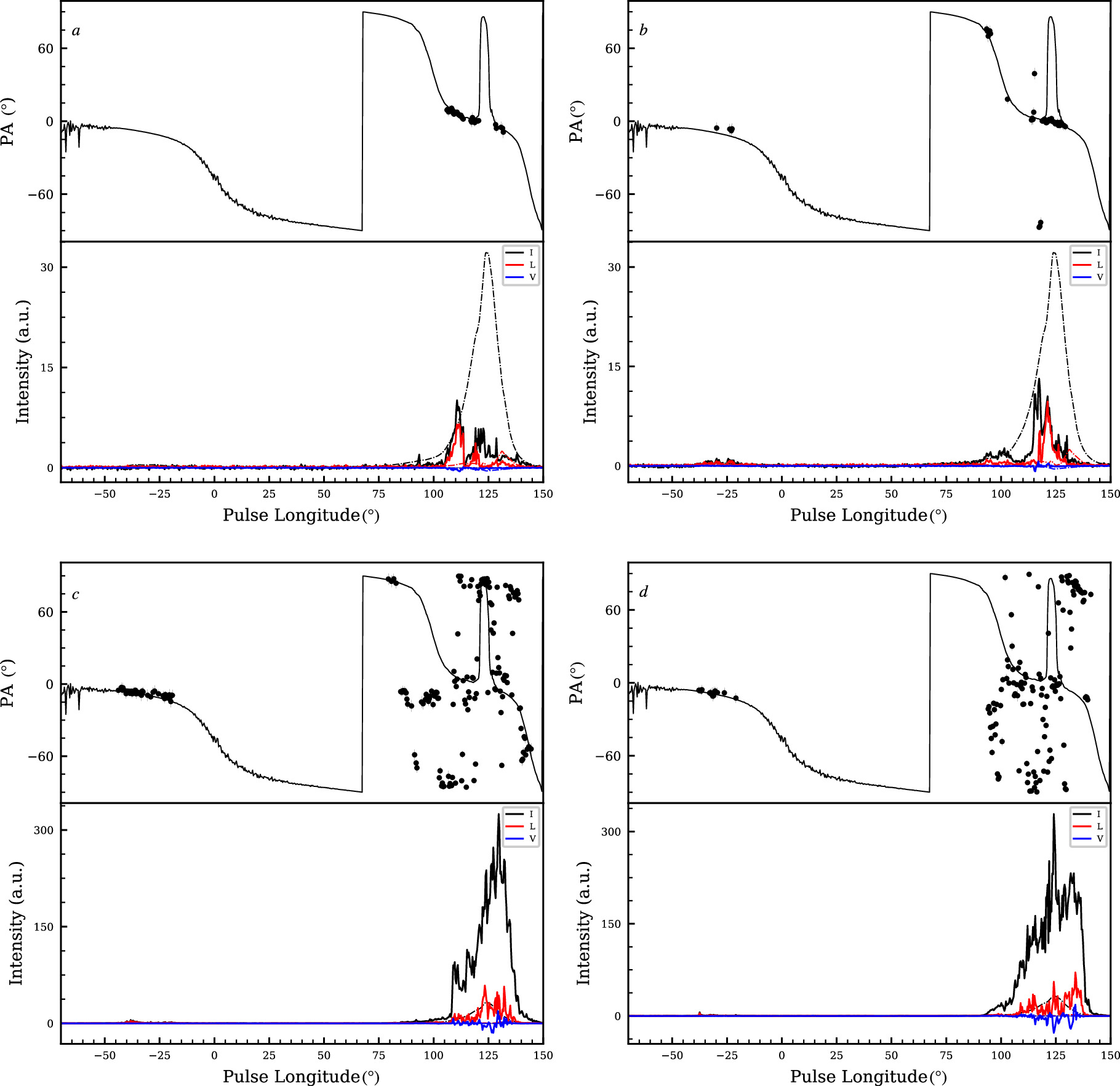

**Figure 9.** The polarization emission features of the sample of four single pulses. In (a), the PPAs of the single pulse are shown as black dots, and the average PPA track is indicated by the solid black line in the top subpanel. Only pulse longitudes with PPA error bars less than 5° for each single pulse are included. The bottom subpanel depicts the Stokes parameter profiles. The total radio emission intensity, the average linear polarization intensity, and the circular polarization intensity are denoted as dashed–dotted black, dashed–dotted red, and dashed–dotted blue curves, respectively.
Download figure:
Standard image High-resolution image

However, it is still worth noticing that in the longitude range from 90° to 100°, the PPA curve of the average pulse profile is steep and looks like an S-shape (in Figures 1 and 8). Also, the single pulses' PPAs in the longitude range from 75° to 100° seem to be another pair of OPMs, with PPA patches separated from the main pulse's PPA patches. The average PPA track in the longitude range from 90° to 100°, along with single pulses' PPA distributed closely around the curve, connects two PPA patches from different pairs of OPMs. Given the discussion above and the fact that one RVM curve could not fit PPAs of both O and X modes at the same time, the RVM does not work in the longitude range from 90° to 100° for the average pulse profile's PPA track. That part of PPAs may indicate a conversion in OPMs, such as the linear coupling between O and X modes discussed in Petrova (2001), which happens when the two modes become indistinguishable.

Compared to the pulse longitudes used in the RVM fit, the main pulse also exhibits a visible contribution from circular polarization, with circular fractions that exceed several times those of the chosen pulse longitudes. This means that circular polarization in the main pulse plays a significant role in the radiation within the magnetosphere. As pointed out by Radhakrishnan & Cooke (1969), the RVM geometry is based on the variation of the orientation of the magnetic field lines with respect to the Ω– μ plane (e.g., the contribution of linear polarization emission to the radiation in the magnetosphere). This model predicts a monotonic rotation of position angle across the pulse profile. Consequently, the observed PPAs of both the single pulse and average pulse in the main pulse deviate from the frame of the RVM geometry due to these polarization emission features. Therefore, the higher contribution of linear polarization emission can reflect the RVM geometry well for this pulsar. In this work, pulse longitudes whose linear fractions are higher than ∼30% are chosen, and the average PPA of the chosen pulse longitudes can be fitted well by the RVM curve.

6. Conclusions

The determination of baseline is one of the key issues in detecting the radio emission polarization of PSR B0950+08 (Wang et al. 2022). In this work, two tentative methods as noted in Equations (1) and (2) are proposed to determine the baseline intensity of this pulsar. After subtracting the baseline intensity with Equation (1), we present the results in Figure 1. The right-hand panel of Figure 1 indicates the inclination angle α = 100 fdg 5 and the impact angle β = −33 fdg 2. The conventional baseline subtraction is also considered, in which the intensity near pulse longitude −100° is chosen as the baseline. The results are shown in Figure 2, which implies the RVM solutions of the inclination angle α = 96 fdg 5 and the impact angle β = −37 fdg 1. Figures 1 and 2 demonstrate that the minimum value of ${\chi }_{\mathrm{reduced}}^{2}$ (the location of the cross) implies similar RVM solutions of α and β, though the set of {α = 100 fdg 5, β = −33 fdg 2} would be more acceptable than the other one due to its low ${\chi }_{\mathrm{reduced}}^{2}$ value, which is about ten times smaller. Moreover, the distribution of the α and ζ values becomes compact in Figure 1. Therefore, the tentative methods described in Equations (1) and (2) would be suitable for determining the baseline of this pulsar characterized by radiation from the whole 360° of longitude.

Figures 1 and 2 indicate also that the polarization emission properties of this pulsar are complex. The main pulse displays depolarization and jumps in position angle, as well as variation in the linear fraction at some pulse longitudes. To obtain the RVM solutions of the inclination angle α and the viewing angle ζ of this pulsar, the pulse longitude ranges from ∼82° to 152° and from ∼−160° to −100° are unweighted in the fit because of low linear polarization fraction and thus large uncertainty of PPAs.

Assuming a magnetic dipole configuration, we could then present the magnetospheric geometry of PSR B0950+08. The three-dimensional view of this pulsar is shown in Figure 3(a). It is found that the curvature radius of the field lines near the magnetic pole becomes very large. Figure 3(b) demonstrates CG (yellow) and AG (gray) regions. In the magnetic dipole configuration, the sparking trajectory responsible for the radio emission of PSR B0950+08 is investigated in the inner vacuum gap model, for both cases of AG and CG, as depicted in Figures 4 and 5. It can be found that the radio emission peak is far away from its magnetic pole. With the AG and the CG models, the calculated emission heights are shown in Figures 6 and 7. These show that PSR B0950+08 is a high-altitude magnetospheric emission pulsar, radiating from heights from ∼0.25R_LC to ∼0.65R_LC (the light cylinder radius R_LC ∼ 12,000 km), and even ∼7800 km for the bridge component.

Acknowledgments

This work made use of the data from the Five-hundred-meter Aperture Spherical Radio Telescope (FAST). FAST is a Chinese national megascience facility, operated by the National Astronomical Observatories, Chinese Academy of Sciences. This work is supported by the National SKA Program of China (2020SKA0120100), the National Natural Science Foundation of China (grant Nos. 12003047 and 12133003), and the Strategic Priority Research Program of the Chinese Academy of Sciences, grant No. XDB0550300.

Appendix: The Determination of the Baseline Intensity of PSR B0950+08

Considering that the pulse profile of the single pulse only occupies a narrow pulse longitude, this emission feature can be used to analyze the baseline response with time for a pulsar with the radiation characteristics of the whole 360° of longitude (like PSR B0950+08). Consequently, compared with the average pulse, the baseline intensity in a single pulse is easily determined. The baseline intensity response with time can be determined by analyzing the baseline position in each single pulse. After eliminating the effect of the baseline response with time, the baseline intensity is a constant over the entire integration, and we assume it as I_b.

For a fixed pulse longitude, its average flux corresponds to the mean intensity of all radio signals along the line of sight over the entire integration time. In different subintegrations, the radio emission intensity of each pulse longitude shows slight fluctuations. This fluctuation may be due to interstellar scintillation. For a pulsar radiating over the whole 360° of longitude, the fluctuation intensity in the strong emission regions (e.g., main pulse) becomes the main influence. The effect of the fluctuation can be eliminated for the pulsar if the integration goes to infinity.

To determine the baseline intensity of the entire 110 minutes observation, the baseline intensity response with time is first taken into account. After eliminating the effect of the baseline intensity response with time, we divide the total individual pulses (N_period) into two equal individual pulses. The number of individual pulses of the first subintegration (from 0 to 55 minutes) is set as N₁. The average radio intensity of this pulsar over the whole pulse phase (i.e., 360° of longitude) is denoted as I_e1 and I_e2 for the first and second subintegrations, respectively. We could have

$\begin{eqnarray}&&{I}_{e1}=\displaystyle \frac{1}{{N}_{1}}\sum _{i{\rm{period}}=1}^{{N}_{1}}{I}_{i{\rm{period}}},\end{eqnarray} \tag{ A1 }$

and

$\begin{eqnarray}&&{I}_{e2}=\displaystyle \frac{1}{{N}_{{\rm{period}}}-{N}_{1}}\sum _{i{\rm{period}}={N}_{1}+1}^{{N}_{{\rm{period}}}}{I}_{i{\rm{period}}},\end{eqnarray} \tag{ A2 }$

where I_iperiod correspond to the pulse of the ith period.

After subtracting the baseline intensity I_b of this observation, we have two average pulse profiles of the intrinsic radio emission of this pulsar over the two equal subintegrations (i.e., I_e1 − I_b and I_e2 − I_b). But I_e1 − I_b is not equal to I_e2 − I_b due to the effect of the fluctuation in emission intensity over different subintegrations. Considering that the average pulse profile of this pulsar is quite stable over long integration, and taking the effect of the fluctuation into account, we find

$\begin{eqnarray}&&{I}_{e1}-{I}_{b}=\kappa ({I}_{e2}-{I}_{b}),\end{eqnarray} \tag{ A3 }$

where κ is a parameter that reflects the fluctuations in the radio emission intensity of this pulsar over different subintegrations.

Radio Pulsar B0950+08: Radiation in the Magnetosphere and Sparks above the Surface

Article metrics

Author e-mails

Author affiliations

ORCID iDs

Dates

Abstract

1. Introduction

2. Observation and Data Reduction

3. Baseline Intensity Determination