


Abstract
While the standard X-ray variability of black hole X-ray binaries (BHXBs) is stochastic and noisy, there are two known BHXBs that exhibit exotic "heartbeat"-like variability in their lightcurves: GRS 1915+105 and IGR J17091–3624. In 2022, IGR J17091–3624 went into outburst for the first time in the NICER/NuSTAR era. These exquisite data allow us to simultaneously track the exotic variability and the corresponding spectral features with unprecedented detail. We find that as in typical BHXBs, the outburst began in the hard state, then continued in the intermediate state, but then transitioned to an exotic soft state, where we identify two types of heartbeat-like variability (Class V and a new Class X). The flux energy spectra show a broad iron emission line due to relativistic reflection when there is no exotic variability, and absorption features from highly ionized iron when the source exhibits exotic variability. Whether absorption lines from highly ionized iron are detected in IGR J17091–3624 is not determined by the spectral state alone, but rather is determined by the presence of exotic variability; in a soft spectral state, absorption lines are only detected along with exotic variability. Our finding indicates that IGR J17091–3624 can be seen as a bridge between the most peculiar BHXB GRS 1915+105 and "normal" BHXBs, because it alternates between the conventional and exotic behaviors of BHXBs. We discuss the physical nature of the absorbing material and exotic variability in light of this new legacy data set.
Export citation and abstract BibTeX RIS

Original content from this work may be used under the terms of the Creative Commons Attribution 4.0 licence. Any further distribution of this work must maintain attribution to the author(s) and the title of the work, journal citation and DOI.
1. Introduction
Black hole X-ray binaries (BHXBs) provide us with opportunities to study different accretion states in a single source on a human timescale. In a typical outburst of BHXBs, they rise from quiescence to a hard state, where the X-ray emission is dominated by emission from the "corona" (the hot plasma with temperature on the order of 100 keV). Then they make a rapid state transition, usually on a timescale of days to weeks (through what is known as the intermediate state), into the soft state, where the disk emission dominates. Finally, they come back to the hard state and then recede again into quiescence (see, e.g., Belloni et al. 2011 and Kalemci et al. 2022 for a recent review). Standard BHXBs show low-frequency quasiperiodic oscillations (LFQPOs; see the review Ingram & Motta 2019 and references therein) in their power spectra. The LFQPOs in BHXBs are usually categorized with an A/B/C classification scheme (see, e.g., Motta et al. 2011). Type C QPOs are strong (≲20% rms) and narrow (Q ≳ 6) and sit on top of a flat-top noise whose high-frequency break is close to the QPO frequency. They are seen commonly in the hard state and hard–intermediate state (HIMS). Type B QPOs are seen in the soft–intermediate state (SIMS), and they are narrow (Q ≳ 6) but weaker compared to Type C (≲5% rms), found usually at 5–6 Hz and sometimes 1–3 Hz. They appear on top of weak red noise. Type A QPOs are very rare, weak (a few percent rms), and broad (Q ≲ 3), and they are accompanied by very weak red noise.
IGR J17091–3624 and GRS 1915+105 are extraordinary BHXBs because they are the only two known BHXBs that exhibit a variety of exotic variability classes, usually consisting of flares and dips that are highly structured and have high amplitudes (e.g., Belloni et al. 2000; Altamirano et al. 2011; Court et al. 2017). Depending on the characteristics of flares and dips, there are distinct variability classes observed: 14 in GRS 1915+105 (Belloni et al. 2000; Klein-Wolt et al. 2002; Hannikainen et al. 2005) and nine in IGR J17091–3624 (Court et al. 2017). Out of the nine classes, seven classes of IGR J17091–3624 resemble those in GRS 1915+105, including the famous "heartbeat" variability, mimicking an electrocardiogram, and the other two are unique to IGR J17091–3624. Because of the famous "heartbeat" class (Class IV in IGR J17091–3624 and Class ρ in GRS 1915+105), in this work, we refer to variabilities that are structured and repeated as "exotic" or "heartbeat-like." It is also worth noting that high-frequency QPOs are detected at the same frequency, 66 Hz, in GRS 1915+105 and IGR J17091–3624 (Morgan et al. 1997; Altamirano & Belloni 2012). The variability in IGR J17091–3624 is generally faster than in the corresponding class in GRS 1915+105 (Altamirano et al. 2011; Court et al. 2017).
IGR J17091–3624 has had eight outbursts in the past 30 yr (see a summary in Section 2.2.26 in Tetarenko et al. 2016). The outbursts in 1994, 1996, and 2001 were identified through an archival search after the first discovery of the source in 2003 (Kuulkers et al. 2003). In both the 2003 and 2007 outbursts, a transition from a hard to a soft state was found, based on spectral and timing properties akin to typical BHXBs (Capitanio et al. 2006, 2009). The following 2011 outburst was the most extensively studied one, and this is when the heartbeat-like variability reminiscent of GRS 1915+105 was observed for the first time in this source (e.g., Altamirano et al. 2011). The mass of the compact object or companion star in IGR J17091–3624 is unknown and no parallax distance is available.
On the other hand, GRS 1915+105 is a 12 ± 2 M⊙ black hole accreting matter from a 0.8 M⊙ K-giant companion in a wide 33.5 days orbit, and the parallax distance to it is  kpc (Greiner et al. 2001; Reid et al. 2014). It is a peculiar BHXB, as it has remained in a persistent bright outburst for 26 yr since its discovery in 1992 (Castro-Tirado et al. 1992), exhibiting a variety of exotic variability classes. In 2018, the source started to fade exponentially and settled in a faint (only a few percent of its previous flux) hard state in 2019 (Negoro et al. 2018; Homan et al. 2019).
While the X-ray variability of BHXB lightcurves is attributed to stochastic and noisy coronal variability, the exotic variability is generally thought to be due to limit-cycle instabilities at the inner accretion disk. The most common hypothesis for the origin of such instability is the radiation pressure instability (Janiuk et al. 2000; Nayakshin et al. 2000; Done et al. 2004; Neilsen et al. 2011). The radiation pressure instability requires the source to accrete at a high Eddington ratio (e.g., >26% LEdd in Nayakshin et al. 2000), which is plausible for GRS 1915+105, as it accretes at above a few tens of percent of its Eddington limit and even super-Eddington rates (Done et al. 2004; Fender & Belloni 2004; Neilsen et al. 2011). However, this hypothesis has been questioned, since similar exotic variability was discovered in IGR J17091–3624. With a flux that is ∼20–30 times lower in IGR J17091–3624 compared to GRS 1915+105, a high-Eddington-accretion scenario means IGR J17091–3624 harbors the lowest-mass black hole known (<3 M⊙ if d < 17 kp), or it is very distant, or the compact object in IGR J17091–3624 is a neutron star (Altamirano et al. 2011).
The disk-wind-jet connections in both GRS 1915+105 and IGR J17091–3624 could shed light on the nature of the exotic variability. In the bright 2011 outburst of IGR J17091–3624, an absorption line at 6.91 ± 0.01 keV was revealed in one Chandra High Energy Transmission Grating (HETG) spectrum, corresponding to an extreme outflow velocity of 0.03c if associated with a blueshifted Fe xxv line (King et al. 2012). Later, Janiuk et al. (2015) noted that in the two Chandra observations in 2011, the presence of absorption lines and heartbeat variability were anticorrelated. These authors proposed that a disk wind might stabilize the disk and suppress the heartbeat pattern. However, Reis et al. (2012) found contradicting evidence, with the discovery of a tentative absorption line at 7.1 keV coincident with the heartbeat variability, using XMM-Newton EPIC-pn data.
In this paper, we present the spectral timing analysis of IGR J17091–3624 in its 2022 outburst using our observing campaign with the Neutron Star Interior Composition Interior Explorer (NICER; Gendreau et al. 2016), the Nuclear Spectroscopic Telescope Array (NuSTAR; Harrison et al. 2013), and Chandra/HETG (Canizares et al. 2005). During this campaign, the source exhibited complex phenomenology, which we attempt to classify into different states based on the spectral and timing properties of the source. After a brief description of the observations and data reduction in Section 2, we begin Section 3 by first describing the methods we use to classify each state. Namely, we identify the different states by (1) the spectral shape and (2) the shapes of the lightcurves. After identifying the different states in Section 3.3, we perform detailed power spectral (Section 4.1) and flux energy spectral analyses (Section 4.2) of each state, to understand how the physics of the accretion flow changes in each state. We summarize the key properties of each state in Section 4.3. Finally, we discuss and interpret our findings in Section 5.
2. Observations and Data Reduction
2.1. Observations
After its last outburst in 2016, IGR J17091–3624 entered a new outburst in 2022 March (Miller et al. 2022). When this outburst began, we triggered our NICER and NuSTAR GO Program (PI: J. Wang). Here, we analyze all 136 NICER observations taken at a near-daily cadence from 2022 March 27 to August 21, as well as six NuSTAR observations taken over this same epoch (see the observation catalog in Table 1). We also requested (by Director's Discretionary Time) one Chandra/HETG observation during this campaign, and this observation took place on June 16, which was simultaneous with the fifth NuSTAR observation. The time evolution of the count rate, fitted disk temperature (see Section 3.1), and the fractional rms are shown in Figure 1.

Figure 1. The time evolution of the NICER count rate (0.3–12 keV, normalized for 52 FPMs), the fitted disk temperature with a baseline model (see Section 3.1), and the fractional rms (0.01–10 Hz in 1–10 keV). There are 305 data points, each representing a 500 s NICER segment used in both the spectral and timing analyses. The color-coding is based on the state identification in Section 3.3. The gray lines indicate when the six NuSTAR observations take place, and the dashed–dotted line marks June 16, during which the Chandra/HETG and the fifth NuSTAR observations take place (see Table 1). Besides MJD, the calendar dates are shown on the top x-axis.
Download figure:
Standard image High-resolution imageTable 1. The Observation Catalog
| State/ | NICER | NuSTAR | ||||||
|---|---|---|---|---|---|---|---|---|
| Variability Class | Date | Exp.(ks) | Counts s−1 | rms (%) | ObsID | Date | Exp.(ks) | Counts s−1 |
| Hard State | 03/14–03/16 | 2.0 | 140 | 27 | ... | ... | ... | ... |
| HIMS | 03/18–03/19 | 10.0 | 562 | 12 | ... | ... | ... | ... |
| SIMS | 03/22–03/27 | 13.0 | 770 | 8 | 80702315002 | 03/23 | 11.3 | 87 |
| 80702315004 | 03/26 | 16.5 | 71 | |||||
| Transition to Class V | 03/27–03/28 | 2.2 | 556 | 16 | ... | ... | ... | ... |
| Class V (exotic) | 03/28–06/30 | 67.5 | 721 | 12 | 80702315006 | 03/29 | 11.9 | 94 |
| Soft State | 03/30–06/26 | 25.0 | 735 | 5 | 80802321002 | 04/21 | 15.1 | 76 |
| Class X (new exotic) | 06/15–07/18 | 19.5 | 648 | 24 | 80802321003 | 06/16 | 16.1 | 69 |
| IMS Return | 07/30–08/21 | 14.5 | 504 | 8 | 80802321005 | 07/31 | 13.9 | 61 |
Note. The source makes excursions between Class V, Class X, and the Soft State from March 28 to July 18, so the dates listed for these three classes are the initial start date and final end date. The exposure times of NICER are the total exposure time of the 500 s segments used in this work, except for that in the Transition to Class V, where we combine all the available data for the flux energy spectrum to increase the signal-to-noise ratio. Otherwise, there would be only two segments of 500 s in the Transition to Class V. The NICER count rate and rms are in 1–10 keV, and the NuSTAR count rate is in 3–78 keV. The Chandra/HETG observation (ObsID 26435) has an exposure of 30 ks and was taken on June 16 in Class X.
Download table as: ASCIITypeset image
2.2. Data Reduction
2.2.1. NICER
We process the NICER data with the data analysis software NICERDAS, version v2020-04-23_V007a, and energy scale (gain) release "optmv10." We use the following filtering criteria: the pointing offset is less than 60'', the pointing direction is more than 30° away from the bright Earth limb and more than 15° away from the dark Earth limb, and the spacecraft is outside the South Atlantic Anomaly (SAA). Data are required to be collected at either a Sun angle >60° or else collected in shadow (as indicated by the "sunshine" flag). We filter out the commonly noisy detectors FPMs #14, 34, and 54. In addition, we flag any "hot detectors," in which X-ray or undershoot rates (detector resets triggered by accumulated charge) are far out of line with the others (∼10σ), and exclude those detectors for the Good-Time Interval (GTI) in question. We select events that are not flagged as "overshoot" (typically caused by a charged particle passing through the detector and depositing energy) or "undershoot" resets (EVENT_FLAGS=bxxxx00), or forced triggers (EVENT_FLAGS=bx1x000), and require an event trigger on the slow chain that is optimized for measuring the energy of the event (i.e., excluding fast-chain-only events, where the fast chain is optimized for more precise timing). A "trumpet" filter on the "PI ratio" is also applied to remove particle events from the detector periphery (Bogdanov 2019). The resulting cleaned events are barycenter-corrected using the FTOOL barycorr. The background spectrum is estimated using the 3C50 background model (Remillard et al. 2022). GTIs with overshoot rates >2 FPM−1 s−1 are excluded to avoid unreliable background estimation. We use the Response Matrix File version "rmf6s" and Ancillary Response File version "consim135p," which are both a part of the CALDB xti20200722. We also add 1% systematics to the NICER spectra at energies below 3 keV to account for the effects of calibration uncertainties. The fitted energy range in the flux energy spectral analysis is 1–10 keV.
2.2.2. NuSTAR
The NuSTAR data are reduced using the data analysis software (NUSTARDAS) 2.1.2 and CALDB v20220802. Due to elevated background rates around the SAA, the data are processed using nupipeline with "saamode=strict" and "tentacle=yes." The source spectra and lightcurves are extracted from circular regions with a radius of  , and the background is from off-source regions of the same size. We also note that stray light contamination is present in the field of view of the focal plane module FPMB in several observations, leading to increased background. Both NICER and NuSTAR spectra are then oversampled in energy resolution by a factor of 3 and are binned with a minimum count of 25 per channel. For the spectral analysis, the fitted energy range is 3–78 keV for NuSTAR observations 1, 2, and 6, and 3–20 keV for NuSTAR observations 3–5, whose spectra are soft, and therefore the background dominates at energies above ∼20 keV.
2.2.3. Chandra
We reprocess the Chandra/HETG data (ObsID 26435) using CIAO v4.14 and CALDB v4.9.7. We follow the standard data reduction process for the grating data and decrease the width of the masks on the grating arms used to extract the spectra from the default of 35 to 18 pixels. This decreases the overlap between the HEG and MEG arms and thus allows us to extend our analysis to higher energies. First-, second-, and third-order spectra were extracted from the observation, and the positive and negative spectra for each order were combined to increase the signal-to-noise ratio with combine_grating_spectra.
All the uncertainties quoted in this paper are for a 90% confidence range, unless otherwise stated. We use XSPEC 12.12.1 (Arnaud 1996) for all the spectral fits. In all of the fits, we use the wilm set of abundances (Wilms et al. 2000), the vern photoelectric cross sections (Verner et al. 1996), and χ2 fit statistics.
3. Methodology for Identification of States
With the nearly daily cadence of our NICER observations, we are able to track the source extensively as it evolved in its spectral and timing characteristics. The phenomenology of IGR J17091–3624 is particularly complex. In this section, we attempt to bring order to this complexity by categorizing the phenomenology and comparing it to previous observations. Here, we present the different methods that we use to describe the phenomenology in each observation, namely, their spectral shapes (Section 3.1) and their lightcurve shapes (Section 3.2), and summarize our findings (Section 3.3). We will then use these state identifications and names throughout the remainder of the paper.
3.1. The Broadband Continuum Shape
To decipher the spectral states, we begin by identifying the dominant spectral component in each observation. In an automated way, we fit the flux energy spectra of all the 305 NICER segments of a length of 500 s (i.e., continuous 500 s intervals), making a total exposure time of 152.5 ks. The baseline model used includes the multicolor disk emission (diskbb) and a Comptonization component (nthcomp). We use cflux to calculate the flux contribution from each component. The XSPEC syntax of the model, therefore, is TBabs(cflux∗diskbb + cflux∗nthComp).
The time evolution of the fitted disk temperature is shown in Figure 1. At the beginning of the outburst, the disk temperature is low (kT ∼ 0.5 keV) and rises to 1.5–2 keV as the luminosity increases. We attempt to place these observations in the conventional hardness–intensity diagram (HID) in order to cleanly identify hard and soft states, but because of these very high disk temperatures and the high galactic absorption column (NH > 1022 cm−2), in some observations more thermal-dominated spectra actually led to larger hardness ratios (e.g., see either hardness ratio in the color–color diagram in Figure 2(b)). In other words, the conventional phenomenological HID fails to capture the corona-dominated states versus the thermal-dominated states. To overcome this, we plot the fitted disk temperature as a proxy for the spectral hardness. 14 The resulting "mimicked" HID is shown in Figure 2(a). With this approach, we can map the evolution of IGR J17091–3624 in its 2022 outburst to more typical BHXBs. Following the classical pattern, IGR J17091–3624 started the outburst in the Hard State (i.e., at low disk temperature, on the bottom right side of the mimicked HID), rose in flux and transitioned to the higher temperatures, corresponding to the HIMS, SIMS, and Soft State, and eventually went back toward the Hard State at a lower flux than the hard-to-soft state transition. This is akin to the hysteresis pattern seen in the HIDs of typical BHXBs.

Figure 2. (a) The mimicked HID showing the spectral state evolution. Both the total flux (1–10 keV) and the disk temperature are measured using the baseline model on the 305 NICER 500 s segments (Section 3.1). The gray arrows indicate the evolution in time. (b) The NICER color–color diagram, where the colors are defined as the count rate ratios between 4–12 and 1–2 keV, and 2–4 and 1–2 keV. The color-coding is based on the state identification in Section 3.3.
Download figure:
Standard image High-resolution image3.2. Lightcurves
Figure 3 shows representative NICER lightcurves discovered during our observing campaign. The shapes of the lightcurves vary dramatically, and these shapes can be broadly characterized into different states (see also Figure 1 for when each state was observed).

Figure 3. Representative NICER lightcurves in each state or variability class. The outburst started in the Hard State, HIMS, and then SIMS (panel (a)), when the variability was stochastic; at the end of the SIMS, exotic variability started to show up (panel (b)); see also the PSD in Figure 4(b)). During the Transition to Class V (e), the heartbeat-like exotic variability developed during 4.5 hr (see further lightcurves in Figure A1). The source then transitioned back and forth between the Soft State (panel (c)), Class V (exotic; panel (f)), and Class X (new exotic; panels (g)–(h)). Finally, the source went back into the IMS Return (panel (d)) when the variability became stochastic again. The count rate is measured in 0.3–12 keV with NICER normalized for 52 FPMs, with time bins of 0.5 s. The NICER ObsIDs are 5202630102 (Hard State), 4618020101 (HIMS), 4618020202 (SIMS), 4618020402 (at the end of SIMS), 5618010403 (Soft State), 5618011401 (IMS Return), 5202630108 and 5202630109 (Transition to Class V), 5202630116 (Class V), and 5618010802 and 5618011202 (Class X).
Download figure:
Standard image High-resolution imageAt the beginning of the outburst (from March 14 to 17), IGR J17091–3624 showed stochastic variability (Figure 3(a); navy curve) that coincided with the hardest spectra, when the disk temperature was at its lowest, at ∼0.5 keV (see also Miller et al. 2022). On March 18, the source flux began to increase, akin to the spectral HIMS (March 18 to 19) and SIMS (March 22 to 27; Wang et al. 2022c), but the variability remained stochastic (Figure 3(a); cyan and green curves). By March 26, exotic variability started to develop in the lightcurves (Figures 3(b) and (e); termed "At the end of SIMS" and the "Transition to Class V"; Wang et al. 2022a), and by March 28, when the disk temperature was near its highest values, between 1.5 and 2 keV (akin to a soft spectral state), the lightcurves showed very clear, structured variability (Figures 3(f)–(h)). The exotic variability seen in panel (f) is reminiscent of the "Class V" variability identified in Court et al. (2017), while the near-sinusoidal variability seen in panels (g) and (h) does not resemble any previously identified classes. Therefore, we term this new variability "Class X " (more details below). From March 28 to July 18, IGR J17091–3624 made excursions between the variability of Class V, Class X, and a more "traditional" Soft State (Figure 3(c)) that shows very little variability altogether.
Here we describe the exotic variability classes in more detail. The structured, exotic variability began gradually at the end of the SIMS, as sharp flares began arising on top of the stochastic variability (panel (b)). Then, on March 27, the lightcurves started to become more variable, with different characteristics than in the SIMS. The NICER lightcurves from March 26 to March 28 are shown in Figure A1. Comparing the lightcurves at March 27 06:10 and 18:49 UTC, the average NICER count rate decreased from ∼800 to ∼600 counts s−1. Later that day, the average count rate decreased even further, to ∼500counts s−1. Then, within 4.5 hr, the source went from demonstrating largely stochastic variability to showing a distinct and highly structured exotic variability pattern, having firmly transitioned to Class V variability (panel (e)).
Class V lightcurves (panel (f)) are characterized as having repeated, sharp, high-amplitude flares, although the period of those flares drifts even within a 500 s segment. Each major flare's apex can be singly peaked or multipronged, the latter of which we refer to as "mini-flares."
The lightcurves in the new Class X (panels (g)–(h)) show nearly sinusoidal variations. They are distinguished from Class V by the larger amplitudes (the mean rms is 24% compared to 14%), uniformity (see the power spectral density, or PSD, in Section 4.1), and symmetry of the flares. Sometimes there can also be additional mini-flares at the peaks of major flares. In some observations, the Class X appeared to nearly vanish, but then reappeared a few hundred seconds later (panel (h)).
Finally, at the end of our campaign (August 21), we observed the source transition back to lower disk temperatures (∼1 keV), akin to a traditional intermediate state, and also the stochastic variability reemerged (panel (d)). We term this state the Intermediate State Return (IMS Return). We note that while our observations stop on August 21, after this date IGR J17091–3624 was found to exhibit exotic variability once again. The analysis of this later behavior will be published in future work.
3.3. Class Identification
From our analysis of the broadband spectral shape (Figure 2), we conclude that this remarkable source transitions between the spectral and timing characteristics of typical BHXBs (e.g., the Hard State, HIMS, SIMS, Soft State, and IMS Return). Then, the shapes of the lightcurves (Figure 3) revealed that there was a phase of Transition to Class V and that sometimes, when the disk component dominates over the corona (as in traditional Soft State), instead of showing very little variability (as in most BHXBs), IGR J17091–3624 can demonstrate exotic (structured and repeated) variability. Therefore, we also identified the exotic variability classes Class V and Class X. In this way, IGR J17091–3624 can be seen as a bridge between the more typical BHXBs and GRS 1915+105, with its famously complex and exotic variability. In the next section, we delve further into the spectral and timing properties of each of these identified states.
As a note to the reader: for the remainder of this paper, we use green/blue/purple colors for observations in the more typical/stochastically varying states (e.g., the Hard State, HIMS, SIMS, Soft State, and IMS Return), while the exotic variability states (Transition to Class V, Class V, and Class X) are shown in red/orange/yellow.
4. Results
4.1. Power Spectra and Dynamical Power Spectrum
To quantitatively investigate the characteristics of the lightcurves, we compute PSDs of all 305 NICER segments of a length of 500 s. We use the "rms-squared" normalization (Belloni & Hasinger 1990), and the Nyquist frequency is 500 Hz. Representative PSDs from each of our identified states corresponding to the lightcurves in Figure 3 are shown in Figure 4. The PSDs in Figure 4 were computed by averaging ≳10 segments of a length of 500 s and are binned geometrically in frequency, i.e., from frequency ν to (1 + f)ν, where f is called the f factor (see Section 2.2 in Uttley et al. 2014 for more details). We choose an f factor of 0.1 to measure the characteristic frequencies more precisely.

Figure 4. Representative PSDs in each state or variability class, which are averaged over ≳10 segments of a length of 500 s to increase the signal-to-noise ratio. The logarithmic frequency rebinning factor is 0.1.
Download figure:
Standard image High-resolution imageAs IGR J17091–3624 can evolve very quickly, on a timescale of a day, we also compute the dynamical PSD (DPSD), to show the evolution of the PSDs over time (Figure 5). The DPSD can be regarded as a matrix of the PSD of each 500 s segment. The DPSD has been color-coded by the identified states, where for a given state/color, the darker shade corresponds to higher variability power. The DPSD clearly reveals the exotic variability, with a peak in the power at around 0.1 Hz, but one can also see other characteristic frequencies popping out.

Figure 5. The dynamical power spectrum using all 305 NICER segments of a length of 500 s in 1–10 keV, color-coded based on the accretion state identification (see Section 3.3 for more details). For a given state/color, the darker shade corresponds to higher variability power, and we only show the gray scale for clarity. The x-axis is the index of the 500 s segments, and we also show the transitional dates on the top x-axis.
Download figure:
Standard image High-resolution imageTo investigate these characteristic frequencies further, we then fit all 305 raw (Poisson noise included) single-segment PSDs with multiple Lorentzian components and a constant for the Poisson noise. The Lorentzians of varying widths describe both the broadband noise and the narrower components (including the "normal" QPOs and the ones caused by exotic variability). We show the characteristic centroid frequencies of the narrower Lorentzian components versus the fractional rms in Figure 6. Below, we describe some of the PSDs in Figure 4 as well as the characteristic timescales for each state and compare to typical BHXBs.

Figure 6. The fitted characteristic frequencies (centroid frequencies of Lorentzians) in the single-segment PSDs vs. the fractional rms (0.01–10 Hz). The NICER energy band used is 1–10 keV. The data points in the Soft State at 5–8 Hz correspond to a highly coherent QPO (see Wang et al. 2024).
Download figure:
Standard image High-resolution imageIn the Hard State (Figure 4(a); navy curve), we detect a QPO at ∼0.3 Hz with a Q factor ∼6 and a fractional rms ∼13%. The QPO is accompanied by a flat-top noise with both low- and high-frequency breaks. The high-frequency break is at a similar frequency to the QPO frequency. These characteristics are consistent with a Type C QPO in a typical hard state.
In the HIMS (Figure 4(a); cyan), both the frequencies of the QPO and the low-frequency break of the flat-top noise increase compared to the Hard State. The QPO is still narrow, with a Q factor ∼6, and its fractional rms is ∼6%. The QPO frequency is in the range of 2.5–5 Hz, and it also anticorrelates with the fractional rms (Figure 6), which is a characteristic of Type C QPOs in normal BHXBs (e.g., see Motta et al. 2011).
In the SIMS (Figure 4(b), green), a narrow and prominent QPO is always present at 2–3 Hz, with a weak power-law noise. No clear correlation between the QPO frequency and the rms can be seen (Figure 6). The Q factor is ∼5 and the rms is ∼5%. These features are consistent with a Type B QPO in the traditional SIMS.
As found in Section 3.2, IGR J17091–3624 transitioned gradually from the SIMS to the exotic Class V, and the PSD in the Transition to Class V has an increase of power generally across frequencies from 0.002 to ∼10 Hz (Figure 4(d)). At the end of the SIMS, because of the consistent Lorentzian centroid frequencies in the segment-based PSDs, we are able to fit the averaged PSD (Figure 4(b)) using the multi-Lorentzian model. We measure the Type B QPO frequency at ν1 = 2.70 ±0.06 Hz and an additional peak at  Hz.
15
The additional peak is caused by modulations occurring with a period of
Hz.
15
The additional peak is caused by modulations occurring with a period of  s (the corresponding lightcurve is shown in Figure 3(b)).
In Class V (Figure 4(e)), the lack of regularity in the flare period produces a PSD that can be fitted with a broad Lorentzian centered in the range of 0.02–0.2 Hz plus a zero-centered Lorentzian for the broadband noise. The centroid frequency anticorrelates with the rms (Figure 6), meaning that when the rms is higher (the variability amplitude is larger), the characteristic exotic variability timescale is longer.
The distinguishable feature of the new Class X (Figure 4(f)) compared to Class V is the uniformity of the flare timescale, which leads to a narrow peak in the averaged PSD at 0.0154 ± 0.0005 Hz, which does not evolve with the rms. There is also a QPO between 2 and 3 Hz, and in the averaged PSD, its centroid frequency is measured to be  Hz. We note that the ∼0.016 Hz and ∼2.7 Hz features at the end of SIMS match, within 90% uncertainties, the frequencies of the features also seen in Class X, although there is a large difference between their rms and PSD shape. This is interesting, because it might indicate some persistent and intrinsic physical timescale in the system. We will discuss this more in Section 5.1.
In the Soft State (Figure 4(c)), the fractional rms is very low (∼6%), and the corresponding PSD is absent of any component besides a weak power-law noise.
In the data set, we discovered a highly coherent QPO with Q factors (defined as the QPO frequency divided by the full width at half maximum) ≳50. The QPO evolved over time, with its frequency ranging between 5 and 8 Hz, appearing first on April 19 and disappearing on June 26 (see Figure 5). When the QPO was present, the PSD consists of the Poisson noise (the PSD is flat over frequency and is consistent with ≃2/〈x〉, where 〈x〉 is the averaged count rate for the rms-squared normalization), red noise (PSD ∝f−2), and an additional noise component that has either a Lorentzian centroid frequency of zero (i.e., flat-top noise) or is in the range of 0.3–0.6 Hz (>3σ away from zero; e.g., see Figure 7). The noise component with nonzero centroid frequency appears as the low-rms extension of the Lorentzian component representing heartbeat-like exotic variability in Class V (see Figure 6). Therefore, for the data with a low total fractional rms ≲6% and a disk-dominated spectrum, we classify them as being in Class V if the centroid frequency for the noise component is nonzero and in the Soft State if the noise component centers at zero. A detailed analysis of the properties and evolution of the highly coherent QPO is presented in a separate paper (Wang et al. 2024).

Figure 7. The PSD that shows the highly coherent QPO. To show both the noise component at low frequencies and the highly coherent QPO, the logarithmic frequency rebinning factor is 0.2 below 3 Hz and 0.025 above 3 Hz. The QPO centroid frequency is fitted to be  Hz, with a Q factor of
  and a fractional rms amplitude of 4.1 ± 0.2% (see Wang et al. 2024 for more details).
Download figure:
Standard image High-resolution imageIn the IMS Return (Figure 4(a), light blue), the PSD is similar to the initial HIMS and SIMS, with flat-top noise and a QPO in the range of 2–6 Hz (Figure 6).
4.2. Spectral Analysis of the Iron K Band
After systematically analyzing the 305 single-segment NICER flux energy spectra (Section 3.1), we combine the NICER spectra in each of our identified states to perform a more detailed spectral analysis, focusing especially on the iron K band. We also include NuSTAR data to cover a broad energy band and to increase the constraining power of the data. Among the eight states, NuSTAR observations are available in all states besides the initial Hard State, the HIMS, and the Transition to Class V (this last state occurred for only one day; see Table 1). The NuSTAR spectra in observations 1 and 2 are combined as they are both in the SIMS.
First, we model the NICER and NuSTAR flux energy spectra in all eight states with the baseline model TBabs∗crabcorr∗(diskbb+nthComp). The model crabcorr serves a NICER and NuSTAR cross-calibration purpose, multiplying each model by a power law with corrections to both the slope by ΔΓ and the normalization (Steiner et al. 2010). The data-to-model ratios are shown in Figure 8. Below, in this section, in order to test the significance level of the iron emission/absorption line, we add a gaussian line with the normalization free to be positive or negative to the baseline model. The energy, width, and normalization of the Gaussian line and the baseline model are all free to vary.

Figure 8. The data-to-model ratio with the baseline model that includes the disk emission and the Comptonization component (see Section 4.2 for more details). Left: the traditional states with stochastic variability, including the Hard State, HIMS, SIMS, and IMS Return, show an iron emission line due to relativistic reflection. Right: the nontraditional states with exotic variability, including the Transition to Class V, Class V, and Class X, show absorption lines from highly ionized iron. The dashed lines indicate Fe Kα at 6.4 keV, He-like Fe xxv at 6.7 keV, and H-like Fe xxvi at 6.97 keV in the NICER spectra and at 6.4 keV in the NuSTAR spectra. The numbers after "Nu" indicate the index of the NuSTAR observation in chronological order.
Download figure:
Standard image High-resolution imageIn the states that are akin to the states in typical BHXBs (i.e., the Hard State, HIMS, SIMS, Soft State, and IMS Return), we see a broad iron emission line in the spectrum, a canonical signature of relativistic reflection. Another signature of reflection, the Compton hump, is clearly detected in the IMS Return (when the hard Comptonized component was strongest). In the Soft State, the broad iron emission line is detected at a significance level of 6σ, measured with NICER and NuSTAR spectra combined.
In the "exotic" states (i.e., Class V, Class X, and the Transition to Class V), we detect absorption lines at energies close to the rest energies of Fe xxv (6.7 keV) and Fe xxvi (6.97 keV). The energies, widths, equivalent widths, and significance levels of the significantly detected absorption lines (>3σ) are shown in Table A1. The 90% upper limit on the blueshift is 0.08 keV, corresponding to an outflow velocity <0.01c. We note that during the Transition to Class V, the absorption lines at 6.7 and 6.97 keV are detected at significance levels of 6σ and 3σ with only a 2.2 ks NICER exposure. The Chandra/HETG observation took place when the source was in Class X. The Chandra/HETG unfolded spectrum and the data-to-model ratio using the baseline model are shown in Figure 9. We measure the Fe xxv and Fe xxvi absorption lines at  and 7.00 ± 0.04 keV with both widths <0.08 keV. The equivalent widths are
  and
and  eV for Fe xxv and Fe xxvi, respectively. The absorption lines are therefore consistent within 90% uncertainty with NICER.

Figure 9. The Chandra/HETG (upper) unfolded spectrum taken in Class X and (lower) the data-to-model ratio with the baseline model. The spectrum exhibits consistent absorption lines with the NICER spectrum (see Section 4.2 for more details). The dashed lines indicate He-like Fe xxv at 6.7 keV and H-like Fe xxvi at 6.97 keV.
Download figure:
Standard image High-resolution imageTable A1. Best-fit Parameters when Fitting the Time-averaged Flux Energy Spectra with the Final Model crabcorr∗tbabs∗(diskbb+nthcomp+relxilllpCp+gauss+gauss+gauss)∗gabs
| Parameter | Epoch 1 | Epoch 2 | Epoch 3 | Epoch 4 | Epoch 5 | Epoch 6 | Epoch 7 | Epoch 8 |
|---|---|---|---|---|---|---|---|---|
| Hard State | HIMS | SIMS | Transition to Class V | Class V | Soft State | Class X | IMS Return | |
| (exotic) | (new exotic) | |||||||
| NuSTAR Obs. | Nu1+2 | Nu3 | Nu4 | Nu5 | Nu6 | |||
| NH | (1.537 ± 0.002) × 1022 cm−2 | |||||||
| a* | 0.998 (f) | |||||||
| i (degrees) | 24 ± 4 | |||||||
| AFe | 1 (f) | |||||||
| Tin (keV) | 0.20 ± 0.02 |

|

|

|

|

|

|

|
| Ndiskbb |

|

| 43.0 ± 0.4 |

|

| 27.6 ± 0.2 | 34.6 ± 0.2 | 60 ± 2 |
| Γ | 1.60 ± 0.02 | 2.033 ± 0.013 |

|

|

|

|

|

|
| kTe (keV) | 100 (f) | 100 (f) | >182 (p) | 100 (f) |

|

|

|

|
| Nnthcomp | <0.02 |

| 0.23 ± 0.01 |

|

| 0.19 ± 0.01 | 0.120 ± 0.003 | 0.23 ± 0.02 |
| h (Rg) |

|

|

| ⋯ | ⋯ |

| ⋯ |

|
| Rin (RISCO) |

|

|

| ⋯ | ⋯ | 1.3 ± 0.1 | ⋯ | 6.2 ± 1.6 |
 (erg·cm⋯−1) (erg·cm⋯−1) |

|

|

| ⋯ | ⋯ |

| ⋯ |

|
 (cm−3) (cm−3) | 18 (f) | 18 (f) |

| ⋯ | ⋯ | 19.8 ± 0.1 | ⋯ |

|
| N relxill (10−3) |

| 9 ± 3 | 12 ± 2 | ⋯ | ⋯ | 0.08 ± 0.02 | ⋯ |

|
| Egauss,1 (keV) | ⋯ | ⋯ | ⋯ |

|

| ⋯ | 6.70 ± 0.03 | ⋯ |
| σgauss,1 (keV) | ⋯ | ⋯ | ⋯ | 0.02 (u) | 0.02 (u) | ⋯ |

| ⋯ |
| Ngauss,1 (10−4) | ⋯ | ⋯ | ⋯ |

| 1.0 ± 0.3 | ⋯ | 1.7 ± 0.5 | ⋯ |
| EW1 (eV) | ⋯ | ⋯ | ⋯ |

|

| ⋯ | 6 ± 3 | ⋯ |
| Significance level1 | ⋯ | ⋯ | ⋯ | 6σ | 5σ | ⋯ | 5σ | ⋯ |
| Egauss,2 (keV) | ⋯ | ⋯ | ⋯ | 7.01 ± 0.04 | ⋯ | ⋯ | 6.97 ± 0.04 | ⋯ |
| σgauss,2 (keV) | ⋯ | ⋯ | ⋯ | 0.02 (u) | ⋯ | ⋯ | 0.02 (u) | ⋯ |
| Ngauss,2 (10−4) | ⋯ | ⋯ | ⋯ | 4.0 ± 1.7 | ⋯ | ⋯ | 1.2 ± 0.5 | ⋯ |
| EW2 (eV) | ⋯ | ⋯ | ⋯ |

| ⋯ | ⋯ | 5 ± 3 | ⋯ |
| Significance level2 | ⋯ | ⋯ | ⋯ | 3σ | ⋯ | ⋯ | 3σ | ⋯ |
| Egauss,3 (keV) | ⋯ | ⋯ | ⋯ | 7.78 ± 0.07 | ⋯ | ⋯ | ⋯ | ⋯ |
| σgauss,3 (keV) | ⋯ | ⋯ | ⋯ | 0.05 (u) | ⋯ | ⋯ | ⋯ | ⋯ |
| Ngauss,3 (10−4) | ⋯ | ⋯ | ⋯ |

| ⋯ | ⋯ | ⋯ | ⋯ |
| EW3 (eV) | ⋯ | ⋯ | ⋯ |

| ⋯ | ⋯ | ⋯ | ⋯ |
| Significance level3 | ⋯ | ⋯ | ⋯ | 3σ | ⋯ | ⋯ | ⋯ | ⋯ |
| Egabs (keV) | 1.74 (f) | |||||||
| σ (keV) | >0.03 |

| 0.05 ± 0.03 | <0.07 | >0.08 | 0.04 ± 0.03 | <0.06 | >0.05 |
| Strength |

| −0.005 ± 0.002 | −0.005 ± 0.002 | −0.004 ± 0.002 |

|

| −0.002 ± 0.001 | −0.009 ± 0.002 |
| ΔΓNICER | 0 (f) | |||||||
| NNICER | 1 (f) | |||||||
| ΔΓFPMA | ⋯ | ⋯ |

| ⋯ | 0.051 ± 0.005 |

| 0.139 ± 0.007 | 0.097 ± 0.004 |
| NFPMA | ⋯ | ⋯ |

| ⋯ | 1.315 ± 0.012 |

| 1.314 ± 0.014 | 1.619 ± 0.011 |
| ΔΓFPMB | ⋯ | ⋯ |

| ⋯ | 0.048 ± 0.006 | 0.111 ± 0.006 | 0.138 ± 0.007 | 0.096 ± 0.004 |
| NFPMB | ⋯ | ⋯ |

| ⋯ | 1.289 ± 0.012 | 1.100 ± 0.012 | 1.290 ± 0.014 |

|
| Disk fraction |
 % % | 5.0 ± 0.5% |
 % % |
 % % |
 % % |
 % % |
 % % |
 % % |
| Flux (10−9 erg cm−2 s−1) |

| 3.25 ± 0.02 |

|

|

|

|

| 3.038 ± 0.008 |
| χ2/d.o.f. | 4516/3857 = 1.17 | |||||||
Note. Errors are at the 90% confidence level and statistical only. The index (f) means the parameter is fixed, (p) means the uncertainty is pegged at the bound allowed for the parameter, and (u) indicates the parameter is unconstrained. The line widths of the absorption lines modeled by gaussian are limited in the range of 0.02–0.05 keV. The line width is set to have an upper limit of 0.1 keV in the phenomenological gabs model. The flux and disk fraction are both measured using cflux in XSPEC in the 2–20 keV band, and the total flux is unabsorbed flux. The equivalent width is calculated using the XSPEC command eqwidth. Even though the model provides a good fit for the spectra, the exact values of the parameters constrained from reflection models that are constrained mostly with the details in the iron line need to be taken with caveats (e.g., the coronal height, black hole spin, and inclination, etc.), because the assumptions in the reflection model used are not guaranteed to hold.
These results indicate that there is a broad iron emission line from relativistic reflection when there is no exotic variability, and there are absorption lines from highly ionized absorbing material when there is exotic variability. Therefore, in our final model, we add to the baseline model (1) a relativistic reflection model relxilllpCp
16
(García et al. 2014; Dauser et al. 2022) for the Hard State, HIMS, SIMS, Soft State, and IMS Return; and (2) absorption lines detected above the 3σ level modeled by gaussian for the Transition to Class V, Class V, and Class X. The best-fitted parameter values are shown in Table A1, and the data-to-model ratios and the unfolded spectra are shown in Figures B1 and 10, respectively. We note that IGR J17091–3624 is a peculiar BHXB with a sometimes very hot disk (Tin can reach ≳1.5 keV), so the assumptions in the reflection model that we use, such as the low-energy break of the Comptonization component, and the geometrically thin disk assumed are not guaranteed to hold (see

Figure 10. The unfolded NICER (left) and NuSTAR (right) spectra using the final model where reflection and absorption lines are included (see Section 4.2 for more details). The dashed lines indicate Fe Kα at 6.4 keV, He-like Fe xxv at 6.7 keV, and H-like Fe xxvi at 6.97 keV in the NICER spectra.
Download figure:
Standard image High-resolution imageWhile the parameters constrained from reflection modeling (e.g., coronal height, spin, and inclination, etc.) warrant caution, they do provide a good description of the reflection features, and therefore the continuum modeling is robust, especially when NuSTAR data are included. We show the parameters describing the properties of the disk blackbody and the corona in each state at different X-ray fluxes in Figure 11. As found in the single-segment NICER spectral fits (Figure 1), the disk temperature is ≲1 keV in the Hard State, HIMS, and IMS Return, and it varies in the range of 1.5–2 keV in the other five states, when the disk fraction is >50%. These five states also have a soft coronal spectrum with a high photon index ≳2, which further solidifies the identification of the SIMS and Soft State, if mapped to the traditional spectral states of BHXBs. We note that the electron temperature of the corona is very low in Class V, Class X, and the Soft State, around 5–10 keV. This has been found also in GRS 1915+105 (e.g., Neilsen et al. 2011).

Figure 11. The parameters describing the properties of the disk and the corona as functions of the X-ray flux with the final model where reflection and absorption lines are included (see Section 4.2). The disk fraction and total X-ray flux are measured in 2–20 keV. The electron temperature kTe cannot be constrained and is fixed at 100 keV in the Hard State, HIMS, and Transition to Class V, and is therefore not shown here.
Download figure:
Standard image High-resolution imageThe global parameters that should not change in time are tied between epochs and, as such, they are constrained with more confidence than the parameters from reflection spectroscopy from individual states. The column density of galactic absorption is constrained to be NH = (1.537 ± 0.002) × 1022 cm−2, consistent with previous measurements (e.g., Xu et al. 2017; Wang et al. 2018). The fitted inclination angle via reflection spectroscopy is  . Previous measurements from reflection spectroscopy using NuSTAR data in the hard state resulted in
  and
and  (Xu et al. 2017; Wang et al. 2018), also suggesting a low inclination for the inner disk producing the reflection.
4.3. A Summary of the Key Properties of Each Accretion State
In Section 3, we describe the broadband continuum shape (i.e., whether it is corona- or thermal-dominated) and the shapes of the lightcurves (i.e., whether they show exotic variability) in order to classify the complex phenomenology of IGR J17091–3624 into eight states. Some of those states are akin to the states in traditional BHXBs (namely, the Hard State, HIMS, SIMS, Soft State, and IMS Return), and then when the source is thermal disk-dominated, it can sometimes take excursions into states with very complex and exotic variability (namely, the Transition to Class V, Class V, and Class X). Here, we summarize the key properties of each of these states, and particularly describe the emission-/absorption-line structure and the PSD structure of each state. The states listed below are given in the order in which they appeared for the first time in this outburst (see Table 1). The quoted measured quantities using flux energy spectra can be found in Table A1.
- 1.Hard State. As in typical BHXBs, the variability in this state is stochastic, with a high averaged fractional rms of 27%, and the PSD consists of a Type C QPO at ∼0.3 Hz on top of flat-top noise. The flux energy spectrum contains a cool disk with disk temperature Tin = 0.20 ±0.02 keV, a corona with a hard spectrum (photon index Γ = 1.60 ± 0.02), and a broad iron emission line due to relativistic reflection.
- 2.H IMS. The variability is still stochastic, while the fractional rms has decreased to 12%. Both the frequencies of the Type C QPO and the low-frequency break of the flat-top noise increase compared to the Hard State. The QPO frequency is between 2.5 and 5 Hz. The disk temperature increases to
 keV and the coronal spectrum is softer than it was, with Γ = 2.033 ± 0.013. The broad iron emission line is present from reflection.
 - 3.S IMS. The fractional rms further declines to 8% and a Type B QPO at 2–3 Hz is present. At the end of the SIMS (March 26), the lightcurve starts to show flares and modulations that are signs of emerging exotic variability on a timescale of s, corresponding to a narrow peak at Hz in the PSD. The disk becomes hotter than it was, with a disk temperature of keV, and the coronal spectrum further softens to . The broad iron emission line is detected in both NICER and NuSTAR spectra.
- 4.Transition to Class V. The lightcurve shows that Class V exotic variability developed over 4 hr in this transitional state, while the flux decreased to half that of the SIMS peak (see Figure 2(a)). Due to this exotic variability, the fractional rms increases to 16%, and the power increases generally across frequencies from 0.002 to ∼10 Hz. The disk is still very hot, with keV, and the coronal spectrum is soft, with Γ > 2.8. Strong absorption lines close to the rest energies of Fe xxv and Fe xxvi are detected at the 6σ and 3σ confidence levels.
- 5.Class V. Exotic flaring variability is evident in the lightcurves. The PSD contains a broad component with centroid frequency in the range of 0.02–0.5 Hz, resulting from the irregularity of the exotic variability. The irregular variability pattern and the broad component in the PSD are similar to Class V in Court et al. (2017), corresponding to Class μ in GRS 1915+105 (Belloni et al. 2000). We will discuss this further in Section 5.1. The averaged fractional rms is 12%. The disk temperature is keV, with a high disk fraction of %, and the photon index is . An iron xxvi absorption line is detected at 5σ confidence.
- 6.Soft State. No exotic variability can be seen in the lightcurves and the averaged fractional rms is only 5%, the lowest among the states. Starting from April 19, a highly coherent QPO appeared (Wang et al. 2024). The disk temperature is keV and the disk fraction is %. The coronal spectrum is soft, with , and an iron emission line is detected at 6σ significance. The low rms, hot-disk domination, and soft coronal spectrum are the features that are in agreement with a traditional soft state (see also the discussion in Section 5.1).
- 7.Class X. Exotic, large-amplitude, near-sinusoidal variability is prominent in the lightcurves, and the fractional rms increases to 24%. The variability amplitude can change within 500 s (see Figures 3(g)–(h)), but the uniformity of the flare timescale leads to a narrow peak in the averaged PSD at 0.0154 ± 0.0005 Hz. This class has never been seen before, in either this source or GRS 1915+105, and we will discuss it more in Section 5.1. With a disk temperature of keV, the disk fraction is %, the highest among all the states. Both Fe xxv and xxvi absorption lines are detected in NICER and Chandra/HETG spectra.
- 8.I MS Return. The variability is stochastic and the PSD shape is similar to the initial HIMS. This state connects the initial HIMS and SIMS in the mimicked HID and color–color diagram (Figure 2). Compared to previous states, the disk temperature has dropped to keV, along with a lower disk fraction of %. The coronal spectrum is still soft, with . Both reflection signatures, the broad iron line and the Compton hump, are prominent in the NICER and NuSTAR spectra.


5. Discussion
5.1. Comparison of Variability Classes
Previously, nine variability classes were defined for IGR J17091–3624 in its 2011–2013 outburst (Altamirano et al. 2011; Court et al. 2017). In this section, we will compare the variability classes we identify for this 2022 outburst with those in previous works.
In the 2022 outburst, we observed Class V identified based on the repeated, sharp, high-amplitude flares in the lightcurves and the PSD shape. We note that a QPO at ∼4 Hz with a Q factor of ∼3 was observed in Class V in the 2011 outburst (Figure 11 in Court et al. 2017). While Class V variability was observed previously, here we see for the first time that the timescale of variability can evolve dramatically, and that it scales with the fractional rms of the source (Figure 6).
We define a new Class X, because of several properties that are different from the previously identified nine classes. Although the uniformity of the exotic variability timescale is reminiscent of the heartbeat class (Class IV in IGR J17091–3624 and Class ρ in GRS 1915+105), the flare patterns are more symmetric than the typical heartbeat (slow rise and quick decay). In the PSD, there is sometimes a QPO at 2–3 Hz, while in Class IV, no QPO was previously detected (Court et al. 2017) or the QPO was at 6–10 Hz (Altamirano et al. 2011). We also find that in Class X, the exotic variability amplitude can vary within even 500 s, while maintaining the variability timescale (see Figures 3(g) and (h)). When the variability amplitude is relatively small, the variability pattern is not only similar to Class III (Class V in GRS 1915+105), but also similar to the end of SIMS, when the source first started to show flares and modulations. The modulation produces a peak in the PSD at ∼0.016 Hz, in addition to a Type B QPO at ∼2.7 Hz. The two characteristic frequencies are respectively consistent within 90% uncertainty at the end of SIMS and in Class X (see Section 4.1 and Figure 6). This suggests that Class X can be regarded as a high-rms extension of the structured variability that starts at the end of SIMS.
We identify the Soft State based upon the lack of exotic variability, the lowest fractional rms of 6%, the hot-disk domination, and a very soft coronal spectrum. There are two classes identified in Court et al. (2017) that also show no exotic variability in the lightcurves—Class I and Class II. The PSD in Class I is similar to the intermediate state here, with a broadband noise at 1–10 Hz and a QPO at ∼5 Hz. We notice the PSD in our Soft State in the NICER hard band 4.8–9.6 keV is similar to the one in Class II using RXTE data (2–60 keV), as both lack any power above ∼1 Hz. However, in our Soft State, the PSD sometimes shows a highly coherent QPO at 5–8 Hz (Wang et al. 2024), which was not detected in Class II.
5.2. IGR J17091–3624 as the Bridge between GRS 1915+105 and Normal BHXBs
In this work, we find that in the 2022 outburst, IGR J17091–3624 went through a traditional hard state and intermediate state, and then entered an exotic soft state, where it sometimes exhibited heartbeat-like variability in the lightcurves. This transition from traditional BHXB states to states showing exotic variability was also suggested in its previous two outbursts in 2011 and 2016 (Pahari et al. 2014; Wang et al. 2018).
In a seminal work, for GRS 1915+105, Belloni et al. (2000) identified 12 variability classes and three basic states and suggested that the variability classes are produced by transitions between the three basic states with certain patterns. Although they found some similarities between the three basic states and the canonical BHXB accretion states, including the soft state and intermediate state, in the variability class GRS 1915+105 spends most of its time in (Class X), the spectrum is the hardest and the lightcurve shows stochastic variability, although it is still not as hard as the canonical hard state of BHXBs. Therefore, the accretion state landscape in GRS 1915+105 is significantly more challenging to understand, due to the more complex phenomenology.
In summary, IGR J17091–3624 shares some variability classes with GRS 1915+105 that are not seen in other BHXBs, while having an outburst recurrence rate (see the summary in Section 1) and evolution pattern in outbursts similar to normal BHXBs. It can therefore be regarded as a bridge between the most peculiar BHXB GRS 1915+105 and normal BHXBs.
5.3. The Nature of Heartbeats
5.3.1. A Brief Review of Radiation Pressure Instability
Although it is generally accepted that the heartbeat-like variability is due to some disk instability, the nature of that instability is unclear. In the standard Shakura–Sunyaev disk, there are two types of instability that might lead to limit-cycle oscillations in the lightcurves: hydrogen ionization instability and radiation pressure instability (e.g., Done et al. 2007; Janiuk & Czerny 2011). The ionization instability takes place in the outer disk and may explain the outburst and quiescence behavior of BHXBs, i.e., lightcurve variability on a long timescale (hundreds of days). On the other hand, radiation pressure instability sets in at a relatively higher mass accretion rate, and thus the inner disk becomes radiation-pressure-dominated. This could then lead to thermal-viscous limit cycles, and is therefore a widely accepted physical mechanism for driving the heartbeat-like variability (Belloni et al. 1997; Janiuk et al. 2000; Nayakshin et al. 2000; Neilsen et al. 2011).
One way to understand the radiation pressure instability is through the "S-curve" when plotting the mass accretion rate  versus the disk surface density Σ at a certain disk radius (e.g., Done et al. 2007). From bottom to top, the S-curve consists of three branches: a stable branch when heating is proportional to the gas pressure balanced by radiative cooling, an unstable branch when radiation pressure dominates (the "Lightman–Eardley instability"; Lightman & Eardley 1974), and another stable branch when advective cooling is effective to balance the heating (the "slim-disk" solution; Abramowicz et al. 1988). That is to say, when the inner disk is radiation-pressure-dominated and
  is on the middle unstable branch, a limit-cycle instability is expected. Over each limit cycle, the mass accretion rate oscillates at each disk radius (switching between the two stable branches), resulting in a "density wave." Observational pieces of evidence supporting this hypothesis include the correlated limit-cycle timescale, disk inner radius (Belloni et al. 1997), and extensive phase-resolved spectroscopic analysis of the heartbeats (e.g., Neilsen et al. 2011; Zoghbi et al. 2016).
We observe a persistent heartbeat timescale of ∼60 s at the end of SIMS and in Class X (see Section 4.1 and Figure 6). A back-of-envelope estimate of the limit-cycle duration is therefore the viscous timescale for the accretion disk (Belloni et al. 1997), which is given by

where M is the mass of the black hole, R is the radius in the disk, Rg is the gravitational radius GM/c2, α is the viscosity parameter, and H is the vertical scale height of the disk (e.g., Frank et al. 2002). A viscous timescale of 60 s can be explained, e.g., by the parameter combination including a black hole mass of 10M⊙, α = 0.03, H/R = 0.1, and R = 46Rg; or, if the black hole mass is 3M⊙, R = 102Rg.
5.3.2. Did IGR J17091–3624 Reach the Eddington Limit?
The Eddington ratio threshold for radiation pressure instability to occur is very uncertain (it could range from 6% LEdd to near Eddington), fundamentally because the S-curve depends on a variety of physical assumptions and conditions (e.g., Honma et al. 1991; Janiuk et al. 2000, 2002). It is therefore natural to find an observational threshold of the Eddington ratio where heartbeats are seen to constrain the underlying accretion disk physics.
So far, heartbeat-like (repetitive, high-amplitude, and structured) variability has been observed in both accreting black hole and neutron star systems and can be a multiwavelength phenomenon. (1) Two BHXBs, including GRS 1915+105 and IGR J17091–3624. In GRS 1915+105, besides X-ray, heartbeat-like variability was also seen in radio and infrared (e.g., Fender et al. 1997; Pooley & Fender 1997). As the mass and distance of GRS 1915+105 are known, it reaches 80%–90% of the Eddington luminosity (Neilsen et al. 2011). (2) Three neutron star low-mass X-ray binaries, including GRO J1744–28 (known as the "Bursting Pulsar"; Kouveliotou et al. 1996; Degenaar et al. 2014), MXB 1730–335 (the "Rapid Burster"; Bagnoli & in't Zand2015), and Swift J1858.6–0814 (Vincentelli et al. 2023). The heartbeat-like (GRS 1915+105-like) variability in neutron stars is also sometimes referred to as Type II X-ray bursts. The luminosity reached near Eddington, ≲20%, and 40% LEdd for the three sources, respectively. We note that the criterion for radiation pressure instability to occur in neutron star systems is when the magnetospheric radius is larger than the neutron star radius (Mönkkönen et al. 2019). This means that the Eddington ratio is not the only key parameter, but also the magnetic field strength. It has been shown that all three neutron star X-ray binaries satisfy this condition for heartbeat-like variability to take place (Vincentelli et al. 2023). (3) An ultraluminous X-ray source in NGC 3621 with an unclear compact object nature (Motta et al. 2020).
The challenging part of finding an observational Eddington ratio threshold then arises—we only have two BHXBs exhibiting heartbeats and for IGR J17091–3624, we do not know the black hole mass (from the mass function) or distance (e.g., from parallax) to estimate the Eddington ratio. The position of IGR J17091–3624 on the radio versus X-ray luminosity diagram suggests a distance between ∼11 and ∼17 kpc for it to lie on the track followed by other BHXBs (Rodriguez et al. 2011). However, it is also possible for IGR J17091–3624 to not follow the typical relation, as was found for GRS 1915+105. A black hole mass in the range of 8.7–15.6 M⊙ is obtained under the two-component advective flow framework (Iyer et al. 2015). On the other hand, there are several BHXBs reaching close to the Eddington limit that do not exhibit heartbeat-like variability (e.g., XTE J1550–564 and 4U 1543–47; Rodriguez et al. 2003; Negoro et al. 2021). Therefore, before the heartbeats in IGR J17091–3624 were discovered, it was proposed that GRS 1915+105 was a unique BHXB that showed heartbeats, because it was the only one that had spent any considerable time above the Eddington limit (Done et al. 2004). Could this also be the case for IGR J17091–3624?
In Figure 12, we show the disk flux Fd versus the disk temperature Tin in the segment-based fits of the broadband continuum (see Section 3.1) in three different states. We also perform fits with the model Fd ∝ Tn (i.e., the disk luminosity L ∝ Tn ), where the power-law index n could indicate the nature of the accretion flow. The standard Shakura–Sunyaev disk predicts L ∝ T4, and the advection-dominated accretion flows including the "slim disk" follow L ∝ T2 (Watarai et al. 2000). We find that in both variability classes showing heartbeat-like variability, the disk luminosity–temperature (L-T) relation is consistent with that of a thin disk (n = 3.7 ± 0.2 and 4.0 ± 0.3 in Class V and Class X). The indication that heartbeat-like variability is associated with a thin disk is consistent with previous conclusions from a theoretical point of view (Nayakshin et al. 2000). We also notice previous phase-resolved spectroscopy of GRS 1915+105 found that the disk forms a loop in the L-T diagram over heartbeat cycles (Neilsen et al. 2011). On the other hand, in the SIMS, the disk has a flatter L-T relation, with n = 1.4 ± 0.3, more in line with a slim disk that is expected at a relatively high Eddington ratio (≳30%; Abramowicz et al. 2010). It is also consistent with n = 4/3 when the mass accretion rate is constant and the disk inner radius is variable, as expected when the local Eddington limit is reached (Lin et al. 2009). In either interpretation of the flatter L-T relation, a relatively high mass accretion rate (≳30% of the Eddington rate) is suggested.

Figure 12. The disk flux (0.1–200 keV) vs. disk temperature Tin in the segment-based fits of the broadband continuum (Section 3.1) in three different states. The dashed lines are the best fits with the model Fd ∝ Tn .
Download figure:
Standard image High-resolution imageIn our observing campaign, we caught the precursor of the heartbeats: the end of the SIMS and Transition to Class V, during which the flux dropped gradually from the SIMS peak to half of that. Considering the suggested slim-disk nature in the SIMS and the idea of the "S-curve," we have a plausible explanation for this precursor behavior. In the SIMS, the inner disk lies on the stable upper branch in the S-curve, which corresponds to the slim-disk solution. Then the mass accretion rate decreased, the inner disk thus entered the middle unstable branch, and heartbeat-like variability (but the variability amplitude is relatively small at the end of the SIMS and is irregular in the Transition to Class V) started to show. Then, in Class V and Class X, the inner disk started to exhibit limit-cycle variabilities, switching between the upper and lower stable branches. The heartbeat-like variability is more structured and regular compared to the precursor phase. The flux in these two classes is also in the middle of the SIMS peak and the Transition to Class V.
The flux peak in the SIMS is near the flux peak in the entire outburst. The measured unabsorbed flux (in units of 10−9 erg cm−2 s−1) at the SIMS peak is ∼8.5 (0.1–200 keV; the flux shown in Figure 2(a) is in 1–10 keV). Assuming that IGR J17091–3624 at the SIMS peak emits at different Eddington ratios, the black hole mass and distance are shown in Figure 13. Based on the coordinates of IGR J17091–3624 (galactic longitude l = 349 52 and latitude b = 221), assuming the distance to the galactic center is 8 kpc, and the radius of the "edge" of the stellar disk in our galaxy is 10–15 kpc (Bland-Hawthorn & Gerhard 2016), the upper limit of the distance to IGR J17091–3624 if it is within the stellar disk is ∼23 kpc. Then, in the case of emitting at 100% Eddington, the black hole mass needs to be <4.3 M⊙. This would make IGR J17091–3624 one of the least massive black holes known. This limit could be brought up to <8.6 M⊙ when adopting a bolometric correction factor of 2.

Figure 13. The black hole mass and distance if IGR J17091–3624 accretes at different Eddington ratios at the SIMS peak when the bolometric flux is ∼8.5 × 10⁻⁹ erg cm−2 s−1. The gray region indicates the distance at which IGR J17091–3624 would be outside of the "edge" of the stellar disk in our galaxy (see Section 5.3.2 for details).
Download figure:
Standard image High-resolution imageAnother empirical benchmark of the Eddington ratio is that the luminosity during the soft-to-hard state transition has a mean value of 2–3% LEdd (Maccarone 2003; Dunn et al. 2010; Tetarenko et al. 2016). As the SIMS peak has ∼two times the flux of the soft-to-hard transition, assuming a slim disk in the SIMS is expected to be ≳30% LEdd, the soft-to-hard transition in this outburst was at ≳15% LEdd, which is ∼1.8σ above the mean value using the standard deviation in Tetarenko et al. (2016).
In summary, our data suggest that IGR J17091–3624 in its 2022 outburst reached a relatively high Eddington ratio because of the L-T relation in the SIMS. Depending on the accretion disk model, this can be, e.g., ≳30% LEdd (Abramowicz et al. 2010), but depends on several parameters, such as the magnetization (e.g., Marcel et al. 2022). We cannot rule out the possibility that IGR J17091–3624 reached a super-Eddington luminosity based on the available black hole mass and distance constraints. Revisiting the conclusion in Done et al. (2004), it is therefore still possible that a super-Eddington luminosity is a necessary condition for heartbeat-like variability to be present. If super-Eddington accretion is a necessary condition, we see new evidence that it alone is not a sufficient condition. In the mimicked HID (Figure 2(a)), the Soft State reaches a similar X-ray flux as the two exotic variability classes (Class V and Class X). This might suggest that it is not just the mass accretion rate that determines whether exotic variability occurs, but rather another factor is required. This other factor could perhaps be the timescale for the inner accretion disk to respond to mass accretion rate changes in the outer disk. We also cannot rule out the possibility that in the Soft State, heartbeat variability is present at other wavelengths rather than X-ray. For example, in Swift J1858.6–0814, the neutron star system where heartbeat-like variability was discovered recently, the heartbeat is most manifest in the infrared band and is much less discernible in X-ray. On the other hand, if IGR J17091–3624 reached only sub-Eddington, it is also a mystery what factor sets IGR J17091–3624 apart from other BHXBs to exhibit heartbeat-like variabilities.
5.3.3. Beyond the Radiation Pressure Instability Model
If the heartbeat-like variability is not related to a high-Eddington-accretion ratio, the known large disk size and the longest orbital period in GRS 1915+105 (33.5 days; Reid et al. 2014) might be the distinguishing factor. In addition, the Bursting Pulsar has a very long orbital period of 11.8 days (Finger et al. 1996). For IGR J17091–3624, one piece of supporting evidence comes from an empirical study of the relationship between the quiescent luminosity and the orbital period (Reynolds & Miller 2011; Wijnands et al. 2012). Assuming this relationship holds, IGR J17091–3624 is inferred to also have a long orbital period of >4 days for a distance of 10 kpc (this can even be tens of days if the distance is actually larger). However, there are several BHXBs with orbital periods longer than 4 days (see Table 13 in Tetarenko et al. 2016). If IGR J17091–3624 indeed has the second-longest orbital period, it has to be ≳480 hr =20 days. Then, if we assume the linear relationship between quiescent luminosity and orbital period holds (the original empirical relationship extends to an orbital period ∼100 hr; Reynolds & Miller 2011), the distance to IGR J17091–3624 inferred is ≳22 kpc, which means IGR J17091–3624 is at its closest on the edge of the stellar disk in our galaxy. In addition, we notice the mechanism that could give rise to heartbeat-like variability in a large accretion disk is not clear. Theory predicts that a longer orbital period corresponds to a larger peak mass accretion rate (Podsiadlowski et al. 2002), and a systematic study of low-mass X-ray binaries has revealed such a correlation (Wu et al. 2010), which relates back to the high-Eddington-ratio scenario. It has also been proposed that the accretion disk in a system with a long orbital period suffers from instabilities in the disk's vertical structure (Życki et al. 1999; Kimura et al. 2016).
Another plausible hypothesis for the heartbeat is disk tearing. In this scenario, if there is initially a tilted accretion disk (a misaligned black hole spin axis and binary orbital axis), Lense–Thirring precession warps the disk, and the disk breaks into discrete rings, each precessing at a different rate. In the hydrodynamical simulation from Raj & Nixon (2021) and Raj et al. (2021), disk tearing leads to mass accretion rate variations that follow a heartbeat pattern. One finding that might support a disk-tearing scenario is that the measured inclination angle from the reflection off the inner disk suggests a lower inclination (∼30°–40°; see Section 4.2), while the disk winds in the soft state of BHXBs are usually expected to be confined to the equatorial plane and therefore in nearly edge-on systems (60°–80°; Ponti et al. 2012). If the low inclination from disk reflection indicates the inner disk inclination and therefore the black hole spin axis, and the high inclination from the high-velocity outflow indicates the outer disk inclination and therefore the orbital axis, this discrepancy might suggest a tilted disk in the system. In GRS 1915+105, Zoghbi et al. (2016) performed spectral modeling over heartbeat cycles and found through reflection spectroscopy that the inner disk inclination varied by ∼10° over a heartbeat cycle, but there is no evidence for misalignment between the inner and outer disk.
5.3.4. Interplay between Heartbeats and Iron Emission/Absorption Lines
One important finding from this NICER and NuSTAR campaign is the interplay between iron emission and absorption lines during this outburst. More specifically, we observe: (1) that in the states that are akin to the typical BHXB states (i.e., the Hard State, HIMS, SIMS, Soft State, and IMS Return), we see a broad iron emission line in the spectrum, a canonical signature of relativistic reflection; and (2) in the "exotic" states (i.e., Class V, Class X, and Transition to Class V), we detect absorption lines at energies close to the rest energies of Fe xxv (6.7 keV) and Fe xxvi (6.97 keV). In this section, we discuss the implications of this interplay between exotic variability and iron emission/absorption lines.
First, we will discuss the wind-driving mechanism. In general, the disk winds in BHXBs could be driven via thermal, radiative, and/or magnetic pressure (see the review in Ponti et al. 2016 and references therein). In the high-Eddington-accretion scenario, high-velocity radiation-driven outflows are expected from the innermost regions. In the disk-tearing scenario (see Section 5.3.3), a magnetically driven wind is seen in general relativistic magnetohydrodynamic simulations of a tilted disk with a high velocity of 0.02–0.2 c launched between 10 and 500 Rg (Liska et al. 2019). In our case, the blueshifts of the significantly detected absorption lines are at most 0.08 keV, indicating a very slow outflow velocity (<0.01c). Therefore, if the wind in this data set is radiatively driven or magnetically driven, as in Liska et al. (2019), the high-velocity component is likely too hot and overionized. Alternatively, the wind may be thermally driven, but the exact relationship between thermal winds and heartbeat-like variabilities is not clear. Thermal winds generally require the inner disk to be able to geometrically illuminate the outer disk, the luminosity to be high enough, and the spectrum to be hard enough that gas in the outer disk can be heated to exceed the local escape speed (Rahoui et al. 2010). If we assume the outflow velocity equals the escape velocity at the wind launching radius, the outflow is launched at a radius larger than 2 × 10⁴ Rg.
Then it becomes puzzling why we do not observe significant absorption lines in the SIMS and Soft State when the flux is at a similar level to the two exotic variability classes. Considering the hinted slim-disk nature in the SIMS (see Section 5.3.2), it is plausible that the corona producing hard X-ray photons cannot illuminate the outer disk with a slim inner disk (the scale height can approach H/R ∼ 1 near the Eddington limit) in the way. We note that studying the role of winds in both IGR J17091–3624 and GRS 1915+105 might be important for understanding the physical mechanism producing heartbeats (see the discussion in Neilsen et al. 2011).
With regard to the emission line, we note that previous phase-resolved spectroscopy analysis has detected an iron emission line in Class ρ of GRS 1915+105 (the traditional heartbeat class; Neilsen et al. 2011; Zoghbi et al. 2016). The absence of an iron emission line from the reflection in the exotic states in this work could be an ionization effect.
5.3.5. Future Directions
The 2022 outburst of IGR J17091–3624 is rich in phenomenology, and provides us with a way of connecting the more typical BHXB evolution to systems that exhibit more exotic variability patterns, but there is clearly more work needed. Besides the spectral timing analysis methods presented in this work, phase-resolved spectroscopy and some novel timing methods, such as recurrence analysis, could shed light on the heartbeat nature. It is worth noting that a deterministic (rather than stochastic) nature of variability resulting from nonlinear dynamics was found in both GRS 1915+105 and IGR J17091–3624 (Suková et al. 2016).
Moreover, the question remains whether IGR J17091–3624 and GRS 1915+105 really are outliers, or perhaps exotic variability is less exotic than we thought. For instance, we found that at the end of the SIMS, there were some flares and modulations that are signs of emerging exotic variability; and some data in Class V could only be identified by the nonzero-centered noise component, but not the lightcurves directly, due to the low level of exotic variability. This data set hints at a rethinking of the canonical state identification of BHXBs that is in general based on the disk and corona contribution to the spectrum and timing features including the total level of variability and QPO properties; perhaps a second dimension perpendicular to the canonical thinking is the level of exotic or nonstochastic variability. It remains an open question if there is a hard boundary between "normal" and "exotic," and if so, where that boundary should be drawn. In other BHXBs, we notice exotic variability that is similar to Class V was discovered in optical in GX 339–4, an archetypical BHXB (Motch et al. 1982), and some "flip-flops" were observed in X-ray in its soft state (Miyamoto et al. 1991; Liu et al. 2022). We note that "flip-flops" are usually associated with state transitions between the HIMS and SIMS and corresponding QPO-type transitions (Types C and B), which have also been found in XTE J1859+226 (Casella et al. 2004) and MAXI J1348–630 (Zhang et al. 2021). In Janiuk & Czerny (2011), the authors searched for heartbeat-like variability using both the lightcurves and any presence of the QPO at a frequency <0.1 Hz and found several candidates showing heartbeats. A systematic search for exotic variability in the multiwavelength lightcurves of both BHXBs and neutron star X-ray binaries will help us understand if this behavior is more common than we realized. The sources we should focus more on are those that reached a high Eddington ratio (XTE J1550–564 and 4U 1543–47), those that have a long orbital period (XTE J0421+560, 1E 1740.7–2942, and GRS 1758–258), or those that have shown interesting variability in the past (GX 339–4, XTE J1859+226, and MAXI J1348–630).
6. Summary
We have presented the spectral timing properties of IGR J17091–3624, the fainter-heartbeat BHXB, in its 2022 outburst, using a legacy data set from NICER, NuSTAR, and Chandra. By aggregating the results using spectral timing tools, including the lightcurves, the PSDs, and the flux energy spectra, our major findings are as follows:
- 1.IGR J17091–3624 first went through a normal hard state and intermediate state. After that, instead of entering a traditional soft state with a stable accretion disk, the flux decreased, and some sort of instability set in, producing heartbeat-like exotic variability in the lightcurve. Then, IGR J17091–3624 transitioned to an exotic soft state, where we identify two types of heartbeat-like variabilities (Class V and a new Class X). Eventually IGR J17091–3624 went into an intermediate state approaching the initial hard state.
- 2.IGR J17091–3624 shares some variability classes with GRS 1915+105 that are not seen in other BHXBs, while having an outburst recurrence rate and evolution pattern in outburst similar to normal BHXBs. It can therefore be regarded as a bridge between the most peculiar BHXB GRS 1915+105 and "normal" BHXBs.
- 3.We observe an iron emission line resulting from relativistic reflection when there is no heartbeat-like variability, and we observe absorption lines from highly ionized iron when there is heartbeat-like variability. This means that whether absorption lines from highly ionized iron are detected is not determined by a soft (disk-dominated) spectral state alone, but rather is determined by the presence of exotic variabilities; in a soft spectral state, absorption lines are only detected along with exotic variabilities. The absorber has an outflow velocity <0.01c, consistent with thermally driven outflows originating from the outer disk.
- 4.We find that although a super-Eddington luminosity in IGR J17091–3624 cannot be ruled out at this point, the luminosity cannot be the only driver of exotic variability, because exotic variability is not always present at the same luminosity.
- 5.If IGR J17091–3624 reached only sub-Eddington luminosities, it remains a mystery what factor sets it apart from the other BHXBs to exhibit heartbeat-like variabilities. Some potential hypotheses involve a large disk size (although the exact mechanism is unclear and might actually relate back to a high Eddington ratio) or disk tearing. In the future, we should systematically search for exotic variability in multiwavelength lightcurves because it might be more common than we realize and some physical mechanism might be shared.
Acknowledgments
We thank Keith Gendreau, Zaven Arzoumanian, Elizabeth Ferrara, Karl Forster, and Pat Slane for scheduling and performing the observations. J.W. acknowledges support from the NASA FINESST Graduate Fellowship, under grant 80NSSC22K1596. J.W. thanks Gibwa Musoke, Megan Masterson, Mason Ng, Navin Sridhar, and Yerong Xu for useful discussions. J.W., E.K., J.A.G., G.M., and M.L. acknowledge support from NASA ADAP grant 80NSSC17K0515. A.I. and D.A. acknowledge support from the Royal Society. M.K. acknowledges support from an NWO Spinoza prize.
Appendix A: Lightcurves at the End of the SIMS and during the Transition to Class V
In Figure A1, we show the NICER lightcurves at the end of the SIMS and during the Transition to Class V, to show in more detail how this transitional phase proceeded. Starting from March 26, we started to observe some flares and modulations that are signs of emerging exotic variability. The more quantitative evidence for this is the peak at low frequencies ∼0.016 Hz in the PSDs (see Figure 4(b)). The spectral and timing features of the data remained very similar until March 27, when we compared the lightcurve at 18:49 UTC to that at 06:10 UTC. The average source count rate decreased from ∼800 to ∼600 counts s−1, with stronger flares and more exotic variabilities showing up. The source count rate continued decreasing to ∼500 counts s−1 on March 27 20:37 UTC. Then, in only 4.5 hr, the source fully transitioned into Class V at March 28 01:01 UTC, with a slightly higher average count rate of ∼620 counts s−1 and much stronger and coherent exotic variability.

Figure A1. The NICER lightcurves at the end of the SIMS (NICER ObsIDs 4618020402 and 5202630108) and during the Transition to Class V (NICER ObsIDs 5202630108 and 5202630109). The dashed line represents the average count rate and the dashed–dotted lines mark the minimum and maximum count rates in the lightcurves shown. The count rate is measured in 0.3–12 keV with NICER normalized for 52 FPMs, with time bins of 0.5 s. The time in each panel marks the start time of the lightcurve.
Download figure:
Standard image High-resolution imageAppendix B: Reflection Spectroscopy Parameters
As we present in Section 4.2, there are relativistic reflection signatures when there is no heartbeat-like exotic variability in the lightcurves. We try to model them with a full reflection model. The parameters in the reflection model are set up as follows. We use the reflection flavor relxilllpCp, assuming a lamppost geometry of the corona. We use a density gradient of a standard α disk (iongrad_type =2), and we take into account the returning radiation (switch_returnrad =1). The BH spin parameter a* is fixed at the maximal 0.998. The global parameters including the Galactic column density NH, the inclination angle, and the iron abundance are tied between epochs. We also add a phenomenological model gabs to account for the residual calibration feature in the NICER spectra at the Si Kα line energy of 1.74 keV. The line energy is fixed, while the width and depth are free to vary among epochs, allowing potential attitude dependency. However, we find the Soft State spectrum drives the iron abundance to be very high at ∼5, while the other epochs showing reflection can be fitted well with a much more physical solar abundance. We thus untie the iron abundance and inclination in the Soft State from the other states and fix the iron abundance at 1 for the other epochs. The disk electron density is difficult to constrain in the Hard State and HIMS, and therefore is fixed at  . The electron temperature of the corona cannot be constrained with NICER alone in the Hard State, HIMS, and Transition to Class V, so it is fixed at 100 keV in those epochs. For Class X, with the highest disk fraction among the eight epochs, it is difficult to constrain the photon index when we use a NuSTAR band of 3–20 keV. We therefore set its lower limit at 2.3, which is the lowest measured for the other epochs besides the Hard State and HIMS.
The resulting data-to-model ratio using the full reflection model is shown in Figure B1. We have discussed the global parameters that are constrained with more confidence and the properties of the disk and corona from the continuum shape in Section 4.2. We notice IGR J17091–3624 is a peculiar BHXB with sometimes a very soft spectrum (dominated by the very hot disk), so the assumptions in the reflection model that we use are not guaranteed to hold (e.g., the low-energy break of the Comptonization component, the assumed geometrically thin disk, and we do not account for emission from the plunging region; see, e.g., Taylor & Reynolds 2018; Fabian et al. 2020). As a consequence, the parameters constrained with reflection spectroscopy need to be taken with caveats. This is especially true for the reflection model included for the Soft State, where both the iron emission line and the Compton hump are weak, and a supersolar iron abundance is required. For the reflection signatures seen in a traditional soft state, it has been found that the irradiation can be dominated by returning radiation from the innermost thermal disk's emission bent by strong gravity (Connors et al. 2021). We choose the same reflection model flavor as the other epochs for the purpose of consistency, but the most appropriate model should be carefully tested in future work. Therefore, we counsel extra caution when interpreting the parameters in the reflection model in the Soft State, including the coronal height, inner disk radius, ionization parameter, and the disk electron density.

Figure B1. The data-to-model ratio of the final model, including the reflection and absorption lines (see Section 4.2 and Appendix B for more details). Left: relativistic reflection is added to the traditional states with stochastic variability. Right: absorption lines are added to the nontraditional states with exotic variability. The dashed lines indicate Fe Kα at 6.4 keV, He-like Fe xxv at 6.7 keV, and H-like Fe xxvi at 6.97 keV in the NICER spectra and 6.4 keV in NuSTAR spectra. The number after "Nu" indicates the index of the NuSTAR observation in chronological order.
Download figure:
Standard image High-resolution imageThe coronal height is low at ≲10 Rg in the Hard State, HIMS, and IMS Return, and it is not well constrained at  Rg in the SIMS. We note this does not formally contradict previous findings from reverberation mapping that the corona expands vertically in the intermediate state, which, however, has usually already started in the HIMS (De Marco et al. 2021; Wang et al. 2021, 2022b). The inner edge of the disk Rin is in the range of 4–7 Rg (Rin is in units of the ISCO radius in Table A1, and to convert to Rg units, a factor of 1.23 corresponding to the assumed maximal a* should be multiplied). If the disk is not truncated (i.e., Rin = RISCO, where RISCO is the innermost stable circular orbit radius that decreases monotonically with a*), this corresponds to relatively low a* between −0.3 and 0.6. This is consistent with the result of −0.13 < a* < 0.27 from reflection spectroscopy using NuSTAR data in the 2016 outburst (Wang et al. 2018).
Footnotes
- 14
We also tried to use the disk fraction (the disk flux divided by the total flux) as the x-axis in the mimicked HID, and found a consistent pattern tracked by the source, but the contribution from the Compton component can be very difficult to constrain with short NICER segments.
- 15
We note that for the standard error on the PSD, we use the formula appropriate for a large number of samples (KM ≳ 20):
, where νj
is the frequency bin and the PSD is averaged over M segments and K frequencies in bin j (Uttley et al. 2014). For one single 500 s segment, the errors on the PSD do not approach Gaussian at frequencies as low as ∼0.016 Hz. Therefore, we average over all 10 segments at the end of SIMS to measure the centroid frequency. - 16
We use relxill v2.2, available at http://www.sternwarte.uni-erlangen.de/~dauser/research/relxill/.

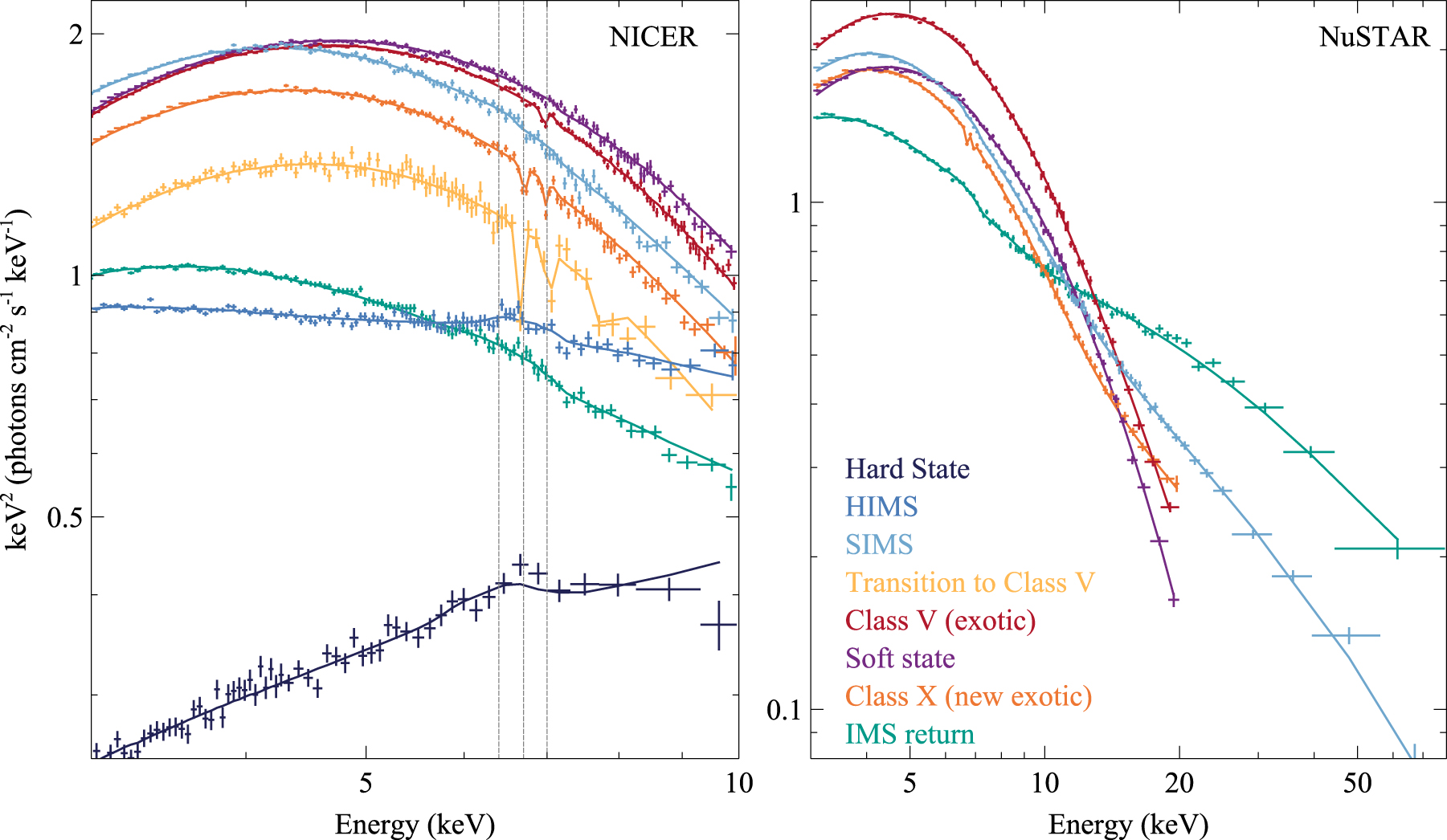
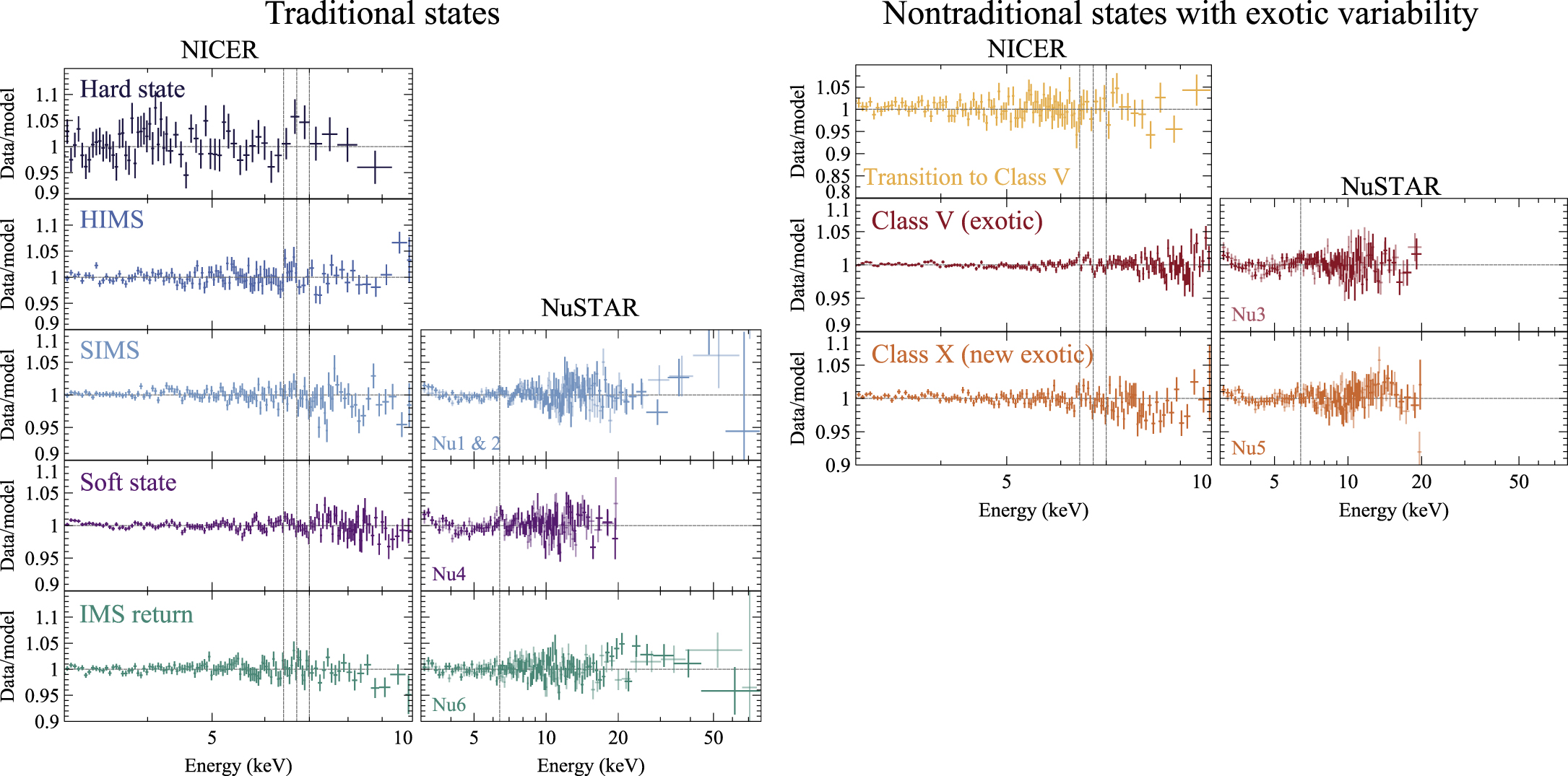