


Abstract
Previous work has established an empirical relationship between densities gained from coronal rotational tomography near the ecliptic plane with solar wind outflow speeds at heliocentric distance r0 = 8R⊙. This work aims to include solar wind acceleration, and thus velocity profiles out to 1 au. Inner boundary velocities are given as a function of normalized tomographic densities, ρN, as ![${V}_{0}=\left(75\ast {e}^{-\left[5.2* {\rho }_{N}\right]}+108\right)$](https://content.cld.iop.org/journals/0004-637X/961/1/64/revision1/apjad1506ieqn1.gif) , and typically range from 100 to 180 km s−1. The subsequent acceleration is defined as
, and typically range from 100 to 180 km s−1. The subsequent acceleration is defined as ![$V(r)={V}_{0}\left(1+{\alpha }_{\mathrm{IP}}\left[1-{e}^{\left(-\left[r-{r}_{0}\right]/{r}_{{\rm{H}}}\right)}\right]\right)$](https://content.cld.iop.org/journals/0004-637X/961/1/64/revision1/apjad1506ieqn2.gif) , with αIP ranging between 1.75 and 2.7, and rH between 50 and 35 R⊙ dependent on V0. These acceleration profiles approximate the distribution of in situ measurements by Parker Solar Probe (PSP) and other measurements at 1 au. Between 2018 November and 2021 September these constraints are applied using the HUXt model and give good agreement with in situ observations at PSP, with a ∼6% improvement compared with using a simpler constant acceleration model previously considered. Given the known tomographical densities at 8 R⊙, we extrapolate density to 1 au using the model velocities and assuming mass flux conservation. Extrapolated densities agree well with OMNI measurements. Thus coronagraph-based estimates of densities define the ambient solar wind outflow speed, acceleration, and density from 8 R⊙ to at least 1 au. This sets a constraint on more advanced models, and a framework for forecasting that provides a valid alternative to the use of velocities derived from magnetic field extrapolations.
, with αIP ranging between 1.75 and 2.7, and rH between 50 and 35 R⊙ dependent on V0. These acceleration profiles approximate the distribution of in situ measurements by Parker Solar Probe (PSP) and other measurements at 1 au. Between 2018 November and 2021 September these constraints are applied using the HUXt model and give good agreement with in situ observations at PSP, with a ∼6% improvement compared with using a simpler constant acceleration model previously considered. Given the known tomographical densities at 8 R⊙, we extrapolate density to 1 au using the model velocities and assuming mass flux conservation. Extrapolated densities agree well with OMNI measurements. Thus coronagraph-based estimates of densities define the ambient solar wind outflow speed, acceleration, and density from 8 R⊙ to at least 1 au. This sets a constraint on more advanced models, and a framework for forecasting that provides a valid alternative to the use of velocities derived from magnetic field extrapolations.
Export citation and abstract BibTeX RIS

Original content from this work may be used under the terms of the Creative Commons Attribution 4.0 licence. Any further distribution of this work must maintain attribution to the author(s) and the title of the work, journal citation and DOI.
1. Introduction
Modeling the evolution of solar wind properties from the solar corona to Earth's orbit is important to advance our understanding of the system scientifically, and to forecast space weather. A major limiting factor for models and simulations is the inner boundary near the Sun. Physical parameters such as density, magnetic field, temperature, and velocity at the inner boundary must be gained or derived from remote observations of the corona, or from model extrapolations of the observed photospheric magnetic field, and large uncertainties in these conditions limit even the most advanced models. Improving, or providing additional, inner boundary conditions can lead to a significant advancement in predicting Earth's space plasma environment, and mitigate the potentially damaging impact of space weather on technology.
The work of Bunting & Morgan (2022) generated an inner boundary condition at distances close to the Sun (8 R⊙) by converting tomographic densities gained via Coronal Rotational Tomography (CRT) into solar wind velocities. The statistical approach was developed further in Bunting & Morgan (2023), through relating densities to velocities at 8 R⊙ via a simple exponential relationship, based on a small number of fitting parameters. This derived velocity distribution was compared to the distribution of in situ velocity measurements made at 1 au, enabling optimization of the fitting parameters. Prior to the comparison, the in situ distribution was reduced by a uniform factor to account, in an oversimplistic way, for the solar wind acceleration between 8 R⊙ and 1 au. The factor we used corresponded to the prescribed acceleration inbuilt to the time-dependent Heliospheric Upwind eXtrapolation (HUXt) model (Owens et al. 2020; Barnard & Owens 2022), which is based on the empirical relation presented in Riley & Lionello (2011). Although giving reasonable estimates of solar wind velocities at 1 au, the velocities derived at 8 R⊙ were incompatible with observations from the Parker Solar Probe (PSP) spacecraft. This was partly due to the HUXt residual acceleration model being optimized between 30 R⊙ and 1 au, and being fixed at a constant value regardless of solar wind type. The bulk of the acceleration occurs at distances close to the Sun (<20 R⊙; Schwenn 1990), therefore there was a significant acceleration that took place below 30 R⊙ that was not properly accounted for in our previous work, and compounded the effect of using the constant HUXt residual acceleration term. This caused an overestimation of the derived velocities at 8 R⊙, particularly for faster solar wind streams.
Heliospheric models drive the initial solar wind conditions at the inner boundary out to 1 au and beyond. Such models traditionally solve three-dimensional magnetohydrodynamic equations, which are computationally expensive. These models, for example the WSA-ENLIL (Wang & Sheeley 1990; Arge & Pizzo 2000; Odstrcil 2003) and HelioMAS (Riley et al. 2012) models, incorporate solar wind acceleration implicitly between distances of 0.1 au (21.5 R⊙) and 1 au. These models also rely on the value of the ratio of specific heat and the solar wind temperature, typically treated as a free parameter at the lower boundary and often poorly reproduced at 1 au. There are many advantages to using simpler, and more efficient models, particularly in the context of requiring large ensembles for space weather forecasting. HUXt is a highly efficient model that adopts a reduced physical approach (see Owens et al. 2020; Barnard & Owens 2022). While solar wind velocities can evolve locally within HUXt as streams of various speeds interact, the overall bulk acceleration of the wind is prescribed as a simple function of distance, with the same relative acceleration set irrespective of the initial solar wind speed (Riley & Lionello 2011; Owens et al. 2020). This is a known weakness of the current implementation of HUXt, since the acceleration profiles of slow and fast solar wind differ considerably, with the fast wind experiencing high acceleration close to the Sun, and the slow experiencing a smaller acceleration that continues to larger distances (Schwenn 1990).
In this work, we introduce acceleration that is dependent on the solar wind initial velocity, and use in situ measurements to constrain the interplanetary velocity profile. In situ observations sunward of the Lagrangian point L1 have been sparse. The Helios mission was the first to send a spacecraft close to the Sun to gain observations of the solar wind. The Helios-B spacecraft reached a perihelion of 0.29 au (∼66 R⊙) in April 1976 (Porsche 1981). This distance was the closest any spacecraft had reached to the Sun until PSP surpassed this distance in 2018 and will continue to a mission perihelion of under 10 R⊙ (Fox et al. 2016). The Solar Wind Electrons Alphas and Protons (SWEAP) package (Kasper et al. 2016) on board PSP takes bulk in situ measurements of the solar wind. The data collected by PSP over several years allows for a detailed investigation of solar wind conditions between the distances of 10 R⊙ and 1 au.
An analysis of PSP in situ measurements to quantify the solar wind acceleration is presented in Section 2. A brief outline of the CRT methodology is outlined in Section 3.1 followed by details of the time-dependent HUXt model. A comparison of the inbuilt HUXt and updated acceleration model is given in Section 3.3. The optimization of the tomographic density to solar wind velocity conversion function is given in Section 3.4. Model results at the location of PSP and Earth are shown in Sections 4.2 and 4.3 respectively. A comparison of model proton densities and temperatures with in situ observations near Earth by the Operating Missions as Nodes on the Internet (OMNI) are presented in Sections 4.4 and 4.5 respectively.
2. Solar Wind Acceleration in the Inner Heliosphere
PSP gives unique observations of the solar wind at distances that regularly vary between perihelion as close as 13 R⊙ and aphelion as far as 1 au. The SWEAP instrument suite makes in situ observations of the solar wind density and velocity at these distance ranges.
The distribution of solar wind velocity with heliocentric distance is shown in Figure 1, which shows PSP SWEAP data taken for all available times between 2018 and 2021 with hourly time binning. The differences in the faster and slower solar wind are clear. The slower solar wind shows a gradual increase in velocity over a much greater distance relative to the fast solar wind. For example the slow solar wind is still noticeably increasing in speed at 150 R⊙ while the fastest solar wind reaches its final velocity at ∼60 R⊙.

Figure 1. Normalized 2D histogram of observed solar wind velocity at the location of the Parker Solar Probe (PSP), binned with heliocentric distance. The data at 1 au are from OMNI data over the same time period with an overlay of HUXt model runs that best fit the acceleration of the fast (red), slow (blue), and mean (green) solar wind.
Download figure:
Standard image High-resolution imageIn the context of solar wind modeling, the overall bulk acceleration (in the absence of local interactions due to stream interactions) must depend on the initial velocity. HUXt uses a simple residual acceleration model with constant parameters, regardless of the initial solar wind velocity (Riley & Lionello 2011; Owens et al. 2020). This work presents a novel acceleration model constrained by the PSP measurements of Figure 1, which we will implement within an adapted HUXt model (Owens et al. 2020; Barnard & Owens 2022).
3. Method
3.1. CRT and Density–Velocity Relations
CRT is a method used to estimate the distribution of coronal electron density. White light coronagraph observations from the CoR2 coronagraph from the Sun–Earth Connection Coronal and Heliospheric Investigation (SECCHI; Howard et al. 2008) suite on board the Solar Terrestrial Relations Observatory (STEREO) spacecraft, are calibrated as outlined in Morgan (2015). A step is then taken to reduce the signals from coronal mass ejections (CMEs) which cause rapid large-scale changes in the density state of the solar corona (Morgan et al. 2012). Finally, the resultant data are passed through an inversion technique based on spherical harmonics outlined in Morgan (2019) to estimate the coronal electron density. This method uses a regularized least-squares regression approach to optimize the tomographic inversion parameters and to best fit the tomographic and observed polarized brightness. The final step narrows the width of structures present in the high-density streamer belt (Morgan & Cook 2020). See Bunting & Morgan (2022) for a more in-depth overview of the CRT method. An example of the tomography density map can be seen in the top panel of Figure 2 for Carrington rotation (CR) 2238 (2020 November). A large archive of tomography maps is available. 3
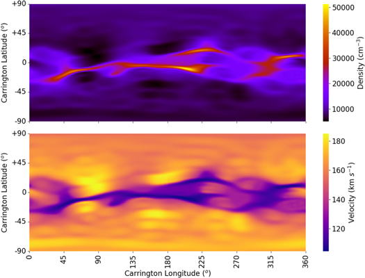
Figure 2. Top: tomographic electron densities of the solar corona; bottom: solar wind velocities (derived from the densities via the method of Section 3.4) at distance 8 R⊙ for CR 2238 (2020 November). These velocities are constrained, or optimized, for the equatorial region only: we cannot quantify the accuracy of values at the mid-latitudes and poles.
Download figure:
Standard image High-resolution imageThe tomographic densities given by the CRT method can be used to estimate the solar wind velocity, which are then used as an inner boundary condition for solar wind models (Bunting & Morgan 2022, 2023). Bunting & Morgan (2022) found that a simple inverse linear density–velocity conversion model generated an inner boundary condition that, when coupled with a heliospheric model, gave model predictions that agreed well with in situ data at 1 au. However, it was found that this method gave inconsistent results. Bunting & Morgan (2023) found that an inverse exponential relationship generated inner boundary conditions that gave more consistent and accurate predictions of solar wind conditions.
In this work, we use the same exponential model outlined in Bunting & Morgan (2023). The tomographic densities are extracted from the equatorial region of the tomography maps at heliocentric distance 8 R⊙. These electron densities give an estimate of the solar wind speeds by

where Vmax and Vmin are scaling parameters for the exponential model, α is a unitless exponential factor, and ρN is the value of the coronal electron density to be converted into velocity, normalized between the minimum and maximum values of density of all available tomographic time periods (2008–2021), namely 4.40 × 103 cm−3 and 5.64 × 104 cm−3.
3.2. HUXt
The time-dependent HUXt model is a lightweight, highly efficient open source heliocentric solar wind model written in Python (Owens et al. 2020; Barnard & Owens 2022). This model ingests solar wind velocities at the inner boundary and propagates solar wind conditions into the heliopshere. The efficiency of this model is increased by assuming an incompressible flow and that pressure gradient, gravitational, and magnetic forces in the solar wind can be negated. This model also solves the solar wind velocities along a single line of latitude, negating non-radial aspects of the ambient solar wind. Despite these assumptions, the model predictions of HUXt over a 40 yr period agree to 6% with full 3D magnetohydrodynamic models (Owens et al. 2020).
Recent advancements have allowed HUXt to perform in three dimensions, as a collection of two-dimensional slices at a range of latitudes (Barnard & Owens 2022). For input, the 3D HUXt requires a "velocity map" which is formed of the velocity state at the inner boundary. The 3D HUXt model becomes extremely useful when extracting predictions at a location that is moving across a range of latitude, such as PSP for example.
3.3. HUXt Acceleration
HUXt adopts a residual acceleration model, in which a velocity V(r) can be calculated at heliocentric distance (r) by
where V0 is the initial velocity at the inner boundary distance (r0), rH is a scale height and αIP is the interplanetary residual acceleration parameter. Riley & Lionello (2011) proposed values of rH and αIP of 50 R⊙ and 0.15 that best matched the HelioMAS model between the distances of 30 R⊙ to 1 au. Within HUXt this acceleration is applied to all inner boundary velocity values independent of magnitude, that is, there is no consideration that slow and fast streams have different accelerations.
Effectively, rH determines the distance at which the solar wind velocity reaches its near-final velocity. The αIP parameter determines the residual percentage increase of the velocity relative to the inner boundary. However, it is known that the fast solar wind accelerates more rapidly and reaches its final velocity at distances closer to the Sun, compared to the slower solar wind as seen in Figure 1 and suggested by previous studies (e.g., Breen et al. 2002; Sanchez-Diaz et al. 2016; Morgan & Cook 2020; Halekas et al. 2022, etc.). In the context of the acceleration model, this suggests that the magnitude of rH and αIP must be dependent on the magnitude of the solar wind velocity at the inner boundary.
Figure 1 demonstrates the effect of varying the rH and αIP parameters on the evolution of the solar wind. The blue, green, and red plots show HUXt radial solutions with different initial velocities at the inner boundary. With increasing initial velocity, rH is increased and αIP is decreased in order to approximate the measured distributions. Due to the intermittent and uneven sampling of the solar wind by PSP at various distances, these profiles have been changed manually to fit, approximately, the slowest and fastest winds, and the most probable intermediate velocities. Parameters for slow, intermediate, and fast streams are listed in Table 1. The blue plot approximates the evolution of the slowest solar wind, green represents the intermediate, and red represents the fastest. The slowest solar wind velocity is still accelerating, albeit gradually, at 1 au (∼215 R⊙) and the fastest solar wind reaches its near-final velocity at ∼150 R⊙. These plots also approximately follow the distribution of the OMNI data at 215 R⊙. In the following work, we alter the HUXt acceleration parameters seen in Equation (2) by linearly interpolating between the rH and αIP depending on the initial solar wind velocities at the inner boundary as listed in Table 1.
Table 1. HUXt Residual Acceleration Parameter (αIP), Scale Height (rH) and Initial Velocity of the HUXt Runs Presented in Figure 1
| Solar Wind Type | Initial Velocity | αIP | rH |
|---|---|---|---|
| (km s−1) | (R⊙) | ||
| Slow | 100 | 1.75 | 50 |
| Mean | 125 | 1.85 | 45 |
| Fast | 180 | 2.70 | 35 |
Download table as: ASCIITypeset image
Examples of HUXt results with a varying inner boundary velocity are shown in Figure 3. In this plot, we show the effect of varying the velocity at the inner boundary on the subsequent evolution of the velocity when the rH and αIP values are interpolated based on values shown in Table 1. As the initial velocity increases, the acceleration between 8 R⊙ and 1 au also increases due to the increasing magnitude of the αIP parameter. Furthermore, the distance over which the velocity increases considerably moves to lower distances due to the decreasing magnitude of the rH parameter.

Figure 3. Evolution of HUXt model velocities with updated acceleration model along a single radial line, with a range of initial boundary condition velocities.
Download figure:
Standard image High-resolution imageSchwenn (1990) analyzed in situ velocity measurements from the Helios mission spacecraft during a period when the Helios-A and Helios-B spacecraft were in radial alignment, showing that the fastest solar wind showed little increase in solar wind velocity between 0.3 and 1 au. This work was later revisited by Maksimovic et al. (2020) who applied a linear acceleration to the solar wind velocity between these heights. The slowest solar wind accelerated at a rate of 90 km s−1 au−1. When a similar approach of a linear solar wind acceleration between 0.3 and 1 au is adopted for the model seen in Figure 3, the slowest solar wind accelerates at a rate of ∼75 km s−1 au−1 over this heliocentric distance range. This provides an improvement on the original HUXt inbuilt acceleration model, which for the same initial velocity at 0.3 au, gave an acceleration of ∼14 km s−1 au−1: a significant underestimation compared to both the findings by Maksimovic et al. (2020) and our PSP-based acceleration model.
3.4. Optimization
As the acceleration of the solar wind is now dependent on the solar wind conditions at the inner boundary, we must now optimize the inner boundary conditions to reflect this. We revisit the tomography-derived inner boundary condition initially proposed by Bunting & Morgan (2022) and further developed by Bunting & Morgan (2023). In the latter study, an empirical conversion function was derived to convert tomographic densities into solar wind velocities at 8 R⊙. However, because of the changes in solar wind acceleration, this inner boundary condition must be re-optimized. As in Bunting & Morgan (2023), we use a quasi-exhaustive fitting method with the aim of optimizing the Vmax, Vmin, and α parameters in the density–velocity conversion seen in Equation (1). In this method, a statistical approach is used to fit the distribution of density-derived velocities to a reduced in situ velocity distribution.
The in situ measurements of velocities are backmapped from 1 au to 8 R⊙; this is done by taking into account the acceleration. We use the updated acceleration model presented in Section 3.3 to find the specific acceleration parameter and, thus, percentage velocity increase between 8 R⊙ and 1 au. We then reduce the in situ measured velocities by this percentage, giving a distribution of expected velocities at 8 R⊙ which is compared to the density-derived velocity distribution. An example of an initial in situ velocity distribution can be seen in the left panel of Figure 4, with the backmapped distribution of the in situ distribution shown in the right panel.
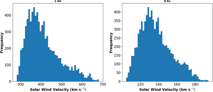
Figure 4. Left: initial in situ solar wind velocity histogram at 1 au; right: reduced in situ (or "backmapped") velocity histogram at 8 R⊙ for the period spanning 2018 November–2021 October.
Download figure:
Standard image High-resolution imageThe fitting method adopts a quasi-exhaustive approach in that, from an initial range of 160–240 km s−1 for Vmax, 80–140 km s−1 for Vmin, and 1–12 for α, optimal values are found. These initial ranges are determined based on the initial acceleration parameters of the model seen in Table 1. Up to this point, the solar wind velocity at 8 R⊙ has been constrained between 100 and 180 km s−1 due to rough extrapolation from the PSP data shown in Figure 1. However, in the context of the fitting method, it is important to allow the fitting algorithm to generate model parameters that give the best possible fit without being strongly constrained on the initial extrapolated values. Therefore, the initial parameter ranges to be tested are chosen to be intentionally wide.
Each parameter range is split into 10 separate bins. We then exhaustively generate a density-derived velocity distribution with every possible combination of the parameter bins. Each modeled distribution is then tested and scored against the backmapped in situ data via the mean absolute error (MAE). The parameter bin which gives the best agreement (lowest MAE) between modeled and backmapped distribution is then chosen and the range is updated to the two adjacent bins for each parameter. This process is repeated until the α bin range becomes less than 0.01 and the Vmax and Vmin parameter ranges become less than 1 km s−1, or until the process has been repeated 11 times (Bunting & Morgan 2023).
4. Results
4.1. Fitting Results
The quasi-exhaustive fitting method presented in Section 3.4 is applied via a sliding window approach, with a "window" of 1 yr's worth of tomography data generating velocities compared with one year's worth of in situ data and a "sliding" in three month increments. Once completed, the average of the fitted values between 2018 October and 2021 September are recorded, and are 5.16 ± 1.09, 183.04 ± 6.13 km s−1, and 107.80 ± 5.45 km s−1 for α, Vmax, and Vmin respectively. The errors are one standard deviation of the values over time.
This result of the fitting process are utilized to generate inner boundary conditions for single CRs. A slice of tomography maps of ±7° from the solar equator is taken. The tomographic densities are then converted into velocities via Equation (1), with the fitted values of α, Vmax, and Vmin stated above. This generates an inner boundary condition that drives a 3D HUXt model run. 3D is chosen instead of the faster 2D model run in order to accommodate the location of the PSP spacecraft. The PSP orbit varies in latitude by over 3° in a single CR. The efficiency of HUXt allows the solar wind velocity to be extracted at any given time at any location with a computational time of only a few tenths of a second. Therefore, to extract and accurately model the PSP spacecraft orbital path, we extract the solar wind velocity at the location of the PSP spacecraft in hourly time steps. The results are presented in Section 4.2. For model predictions at the location of Earth, a 2D HUXt run is used. The comparison of modeled velocity and in situ OMNI data is presented in Section 4.3.
4.2. PSP Results
The time series comparison between PSP observational data (orange) and modeled velocity (blue) at the location of PSP is shown in Figure 5. There is a strong correlation between the observed and modeled velocities at PSP for all time periods. The model accurately predicts prolonged periods of relatively slow solar wind (2019 March–April) as well as periods of more variable solar wind conditions (2020 December–2021 February). The statistical analysis are promising, with an MAE of 64.3 km s−1 and root mean square error (RMSE) of 87.8 km s−1. This provides an improvement on the density–velocity-derived inner boundary condition optimized for the inbuilt acceleration of HUXt (Bunting & Morgan 2022), with the point-to-point metrics of these data being 64.8 km s−1 for MAE and an RMSE of 92.7 km s−1 over the same time period. These suggest that the tomography–HUXt model, with the updated acceleration model, provides a reasonable estimate of the solar wind conditions at heliocentric distances less than 1 au. Further statistics can be found in Table 2. The small-scale variations in the PSP data closely align with the general trend predicted by the model, with the general magnitude of the fast solar wind streams (e.g., 2018 November) showing a good agreement. Also, modeled periods of uncharacteristic slower solar wind (2021 August) demonstrate a good estimation of the in situ data. Due to the data gaps, it is difficult to suggest that the model predicts the solar wind conditions well for all times, but certainly something can be said for the strong agreement during periods where PSP data are recorded.
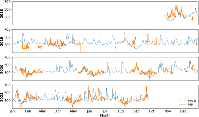
Figure 5. Model predictions vs in situ data at the location of PSP.
Download figure:
Standard image High-resolution imageTable 2. Statistical Analysis of Model Output with OMNI Data at 1 au and PSP Data for Inner Boundary Conditions Optimized on the Inbuilt and Updated Acceleration Models
| Acceleration Model | Position | MAE | RMSE a | PCC b |
|---|---|---|---|---|
| (km s−1) | (km s−1) | |||
| Inbuilt c | PSP | 64.8 | 92.7 | 0.405 |
| Earth | 55.5 | 76.8 | 0.527 | |
| Updated | PSP | 64.3 | 87.8 | 0.445 |
| Earth | 52.8 | 72.4 | 0.514 |
Notes.
a Root mean square error. b Pearson correlation coefficient c See Bunting & Morgan (2022).Download table as: ASCIITypeset image
Figure 6 shows a direct comparison between the model velocities at the location of PSP with heliocentric distance at the same times as shown in Figure 1 for models optimized using the inbuilt acceleration model as presented in Bunting & Morgan (2023) in (b) and optimized on the updated acceleration model shown in (c).
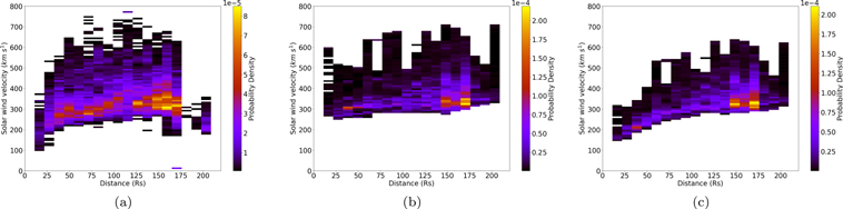
Figure 6. Normalized histograms of the solar wind velocities at the location of PSP for in situ observations (a); modeled velocities at the location of PSP for (b) the inbuilt acceleration model and (c) the adapted acceleration model.
Download figure:
Standard image High-resolution imageThe difference between the two acceleration models are demonstrated clearly in Figure 6. The adapted acceleration model histogram (Figure 6(c)) shows a strong noticeable increase in velocity with distance when compared to the inbuilt histogram (Figure 6(b)). A comparison between the two histograms shows that the velocity distributions at greater heliocentric distances agree. This is expected as both models are optimized on gaining velocity distributions at 1 au. However, the differences become more obvious at smaller distances. The inbuilt acceleration model gives a minimum velocity at the inner boundary of around 250 km s−1 while the adapted acceleration model gives velocities that rarely exceed 220 km s−1.
When the adapted acceleration model histogram (Figure 6(c)) is compared to the in situ data shown in Figure 6(a), the modeled data show a stronger concentration of slower solar wind velocities, specifically in the bins between 110 and 120 R⊙. However, there are areas where the higher solar wind values seem to better match the range of velocities seen in Figure 6(a)), specifically ∼150 R⊙ and greater. This is again due to the density–velocity conversion model being optimized for measurements at 1 au. Overall, the adapted acceleration model gives a distribution that gives far better agreement with PSP measurements in comparison to the inbuilt acceleration model.
4.3. Earth Results
The prime focus of space weather forecasting is accurately predicting the solar wind conditions at Earth. In this section, the model predictions at Earth are tested against in situ data provided by OMNI and processed as stated in Section 3.4. The densities are extracted at the latitude of Earth only. The tomographic densities are then converted into velocities at 8 R⊙ and used as an inner boundary condition for HUXt. Figure 7 shows the model predictions (blue) compared to the in situ solar wind velocities (black) at Earth.
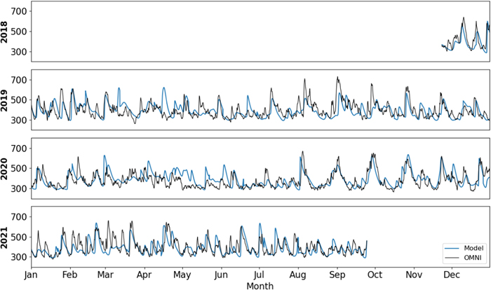
Figure 7. Comparison of model predictions (blue) and in situ solar wind velocities provided by OMNI (black).
Download figure:
Standard image High-resolution imageFigure 7 shows that the model makes a good estimate of the ambient solar wind conditions at Earth. There are periods of excellent agreement both in terms of time of arrival and magnitude of the faster solar wind streams, such as the majority of 2021, and 2020 August–December. Statistically, the model provides good predictions of the solar wind conditions at 1 au with an MAE of 52.8 km s−1 and RMSE of 72.4 km s−1. Further statistics are provided in Table 2. There are periods where a fast solar wind stream is observed, but not predicted, by the model such as July 2020. Short periods of disagreement could be due to CMEs in the measurements that are not included in the model. There are occasions which the model predicts a fast solar wind stream that is not observed by OMNI. The main source of error is defects in the tomography density maps, including latitudinal uncertainty. As seen in Figure 2, there are steep gradients in density within the solar corona at the boundary between the equatorial streamers and coronal holes. A small latitudinal or longitudinal inaccuracy in the tomography model, or small deflections of streamers with distance, will cause a large inaccuracy in the boundary velocity, and a subsequent large error in the model solar wind velocity.
4.4. Mass Flux Conservation
Given the modeled velocity profiles, and the tomographical densities at 8 R⊙, we use mass flux conservation to propagate densities to 1 au by
where ρ and V are density and velocity at heliocentric distance r. The 0 subscript indicates the inner boundary and the 1 subscript indicates 1 au.
An example of the evolution of the solar wind velocity and proton density is shown in Figure 8. This is shown for two cases showing an example of typical slow solar wind (blue) V0 = 118 km s−1, and typical fast solar wind (red) V0 = 180 km s−1. As well as the clear anti-correlation between density and velocity, Figure 8 also shows that, in the case of the fast solar wind, the density is close to a factor of 10 smaller than that of the slow solar wind. This agrees with other models and observations (e.g., Habbal et al. 1997; Schwenn 2006; Allen et al. 2020; Bunting & Morgan 2022).
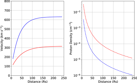
Figure 8. Left: solar wind velocity as a function of distance for a typical case of fast (V0 = 180 km s−1, blue) and slow (V0 = 115 km s−1, red) solar wind. Right: corresponding proton densities derived via mass flux conservation.
Download figure:
Standard image High-resolution imageAs this approach is applied to the modeled values at the inner boundary and 1 au, a back-mapping approach is used in order to directly relate the same parcel of plasma at the two distances of interest. This back-mapping approach entails ejecting and tracking "test particles" within the HUXt model at the inner boundary in 5° increments. The time taken for the test particles to reach 1 au is recorded and the differences in time of arrival, along with knowledge of the solar rotation rate set by HUXt, allow a longitudinal shift to be calculated and build a relationship between the parcels of plasma at 1 au and the inner boundary.
Once the back-mapping approach is undertaken, a post-processing step is applied to ensure there is no crossing of solar wind streams. This allows the electron density at 1 au to be derived from the tomographic densities and derived velocities via Equation (3). We convert the electron density to proton density by assuming a 90% composition of ionized hydrogen and 10% ionized helium is for a quasi-neutral solar wind. Therefore, the relative abundance between the two species is 9 H+ : 11 e−. This is used for the final comparison between modeled and observed proton densities which can be seen in Figure 9 with accompanying point-to-point metrics seen in Table 3.
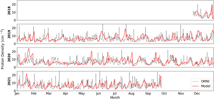
Figure 9. Mass flux solutions of proton density at 1 au (red) compared with in situ measurements from OMNI (black).
Download figure:
Standard image High-resolution imageTable 3. Statistical Analysis of MAE, RMSE, and PCC between Modeled and Observed Proton Densities at 1 au
| Position | MAE | MSE | RMSE | PCC |
|---|---|---|---|---|
| (cm−3) | (cm−6) | (cm−3) | ||
| Earth | 2.91 | 15.70 | 3.70 | 0.375 |
Download table as: ASCIITypeset image
There is a strong correlation between the general trends of the in situ and modeled proton densities presented in Figure 9. Statistically both compare with an MAE of 2.9 cm−3 and a Pearson Correlation Coefficient of 0.38. These results also give confidence that the tomographic densities are accurate and that our velocity model is a good representation of the solar wind. However, the sharp peaks in proton density observed by OMNI are not all present within the modeled densities. One reason for this is that HUXt provides a relatively smoothed velocity output (see Figure 7), due to the resolution requirement of the model input. The inner boundary consists of a coronal resolution of ∼2 8. Thus, HUXt is restricted to resolving solar wind structures at Earth with an approximate 8 hr resolution. The reduced physical approach could also introduce discrepancies in the output here when accurately modeling the compression and rarefraction present in a stream interaction region.
4.5. Proton Temperature
Profiles of velocity and density allow for an estimate of proton temperatures. For this, the force equation that describes a steady-state flow of the solar wind through infinitesimal radial tubes is used (Munro & Jackson 1977):

where  is the pressure gradient, G is the gravitational constant, M⊙ is solar mass, and ρ
D represents the outward force per unit volume on the plasma possibly due to wave–particle interactions. In the following work, we only consider gas pressure and gravitational forces, thus D = 0. Substituting the ideal gas law into Equation (4) gives
is the pressure gradient, G is the gravitational constant, M⊙ is solar mass, and ρ
D represents the outward force per unit volume on the plasma possibly due to wave–particle interactions. In the following work, we only consider gas pressure and gravitational forces, thus D = 0. Substituting the ideal gas law into Equation (4) gives

where μ is the mean atomic weight (∼0.62), mp is the proton mass, kB is Boltzmann's constant, and Tp is proton temperature.
We now consider two typical cases of the solar wind: fast and slow. The relationship of velocity and density of these cases can be seen in Figure 8. The fast solar wind case shows an initial velocity (V0) of 180 km s−1, which accelerates to ∼620 km s−1 at 1 au. In the case of the slow solar wind, the velocity at the inner boundary is 115 km s−1 which accelerates to ∼300 km s−1 at 1 au.
For each of these two cases, the above parameters of ρ and V are used to derive a fitting parameter (rhs of Equation (5)). Using an iterative process, a function of Tp with distance is found that gives the best agreement of the rhs of Equation (5) to the fitting parameter. With the aim of generating a more stable fit, the log of the negative of the rhs of Equation (5) is fitted. The fitted parameters of each case can be seen in the dotted red (slow) and blue (fast) plots in the left panel of Figure 10.
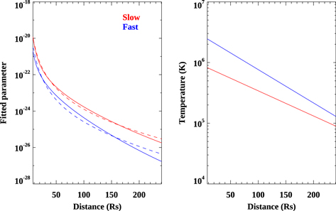
Figure 10. Left: fitting parameter used to gain the proton temperature. Right: fitted function of proton temperature with heliocentric distance.
Download figure:
Standard image High-resolution imageA scale-height function of Tp gives a stable agreement to the fitted parameter, given by
where T0 and H0 are free parameters and h = r − r0.
In the case of the fast (slow) solar wind, T0 was found to be 2.5 ×10⁶ K (8.2 ×10⁵ K) and H0 had a magnitude of 79.0 R⊙ (104.7 R⊙). Proton temperature (Tp ) is shown as a function of distance in the right panel of Figure 10.
These results show that fast solar wind has a greater temperature, and aligns more closely with in situ measurements, than in previous studies (e.g., Feldman et al. 1974a, 1974b). Measurements of solar wind temperature have been performed by analyzing ionized helium temperatures from the Helios spacecraft at a range of heliocentric distances between 0.3 and 1 au. Marsch et al. (1982) found that the radial temperature of a parcel of faster solar wind (∼650 km s−1 at 1 au) had an initial temperature of 1.3 MK at ∼65 R⊙, decreasing to 0.9 MK at 1 au. Figure 10 finds a temperature of ∼1.5 MK at ∼65 R⊙, decreasing to 0.2 MK at 1 au. Likewise for a parcel of slow solar wind (solar wind speed of ∼350 km s−1 at 1 au), Marsch et al. observed a temperature of 0.35 MK at 65 R⊙, cooling to 0.15 MK at 1 au. Figure 10 shows a temperature of 0.5 MK at 65 R⊙, cooling to 0.15 MK. This comparison shows that the model is reasonable for the slow solar wind, but the fast solar wind temperature is greatly underestimated at greater heliocentric distances compared to the work of Marsch et al. (1982). There are two major reasons for this disagreement: (1) the work presented above neglects the wave pressure term which could be significant in heating the faster solar wind (van Ballegooijen & Asgari-Targhi 2016); (2) protons are expected to have a strong temperature anisotropy whereas the above work assumes an isotropic solar wind (Huang et al. 2020).
Elliott et al. (2012) used a statistical approach to derive a relationship between proton temperature and solar wind velocity within the ambient solar wind observed by OMNI. A quadratic relationship gave a good representation between proton temperature and velocity at 1 au. The results suggest a parcel of solar wind traveling at 620 km s−1, such as the example given in Figures 9 and 10, yields a temperature of ∼1 ×10⁵ K, agreeing with our temperature model. Likewise for the slow solar wind case, Elliott et al. (2012) suggested a velocity of 300 km s−1 at 1 au corresponds to a proton temperature of ∼2 × 10⁴ K. This value is significantly lower than our estimation (9 × 10⁴ K).
5. Discussion
We base the acceleration profile of the solar wind on in situ observations provided by the PSP spacecraft. Previous models have estimated the solar wind velocity profile of the inner heliosphere with methods derived from both theory and in situ observations. Burlaga (1967) introduced a power-law acceleration model derived from a solution of the Parker model (Parker 1958). The power-law fit ("Parker fit") is described as Vr (r) = ar1/4 where a is a constant. Alternatively, Venzmer & Bothmer (2018) re-analyzed in situ observations during a period of alignment between Helios-1 and Helios-2 spacecraft initially presented in Schwenn (1990). Venzmer & Bothmer (2018) suggested a median velocity profile ("VB18") constrained to the heights of 0.3–1 au, by binning the in situ observations by r. The median velocity profile is described by: Vrmed(r) = Kr0.099 where K is a constant. Following the work by Macneil et al. (2022), in which observed heliospheric current sheet crossings at 215 R⊙ were mapped back to Potential Field Source Surface (PFSS) solutions at 2.5 R⊙, a value of a and K are chosen to constrain the solar wind velocity to 400 km s−1 at 1 au. To provide a comparison with these previous results, we run HUXt for both the inbuilt and the updated acceleration to yield a solar wind velocity of 400 km s−1 at 1 au. Comparisons of velocity profiles between 8 R⊙ and 1 au are shown in Figure 11.
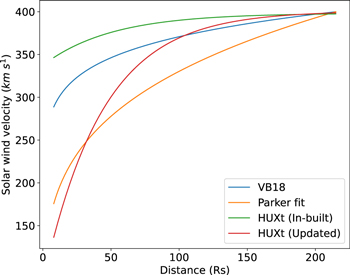
Figure 11. Velocity profile between the heights of 8 R⊙ and 1 au for the fitted Parker model (orange), the VB18 model (blue), the inbuilt (green), and updated (red) HUXt acceleration models.
Download figure:
Standard image High-resolution imageFigure 11 shows that the VB18 model (blue) and the HUXt inbuilt (green) model velocities are comparable, albeit with a more gradual increase for the latter. Due to the orbital constraints of the Helios spacecraft, the VB18 model is constrained by observations between 8 and 30 R⊙, which can explain why the VB18 velocities of ∼300 km s−1 at 8 R⊙ do not agree with PSP observations. This supports the findings of Macneil et al. (2022), suggesting that a more impulsive acceleration is necessary compared to the gradual form produced by both the Parker model and the existing HUXt implementation. The updated HUXt velocity profile (red) provides a reasonable agreement with the Parker solution (orange), although the Parker solution has a far more gradual increase in velocity profile.
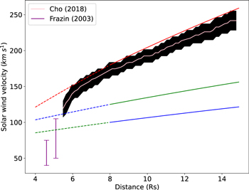
Previous acceleration models at low heliocentric distances have been undertaken via a range of methods. Frazin et al. (2003) analyzed the outflow speeds in equatorial streamers using Doppler dimming of O5+ ions measured by the Ultraviolet Coronagraph Spectrometer instrument on board Solar and Heliospheric Observatory (SOHO; Kohl et al. 1995) at 4.6 and 5.1 R⊙ (see Figure 12, purple). At distances of 6–16 R⊙ Cho et al. (2018) applied a Fourier correlation filter to Large Angle Spectroscopic Coronagraph C3 (Brueckner et al. 1995) data, with their average speeds over the year 2009 shown in Figure 12 (pink with ± 1 σ shown in gray). Figure 12 compares the studies mentioned above to the "slow" (blue), "mean" (green), and "fast" (red) solar wind HUXt runs shown initially in Figure 1, with extrapolation to distances less than 8 R⊙.
Figure 12. Comparison of solar wind acceleration from HUXt runs seen in Figure 1 with Cho et al. (2018) and Frazin et al. (2003). Dashed plots represent inward mapping of HUXt runs from 8 R⊙ to 4 R⊙ via Equation (2).
Download figure:
Standard image High-resolution image
Figure 12 shows a strong agreement between the velocity values derived by Cho et al. (2018) and our "fast" model. The "mean" and "slow" models are significantly lower than that of Cho et al. (2018). The comparison to the work presented in this study suggests that the data presented in Cho et al. (2018) were dominated by fast solar wind, which is expected as 2009 corresponds to solar minimum and the streamer belt being confined to a narrow region near the equator.
The comparison of the HUXt model to the work by Frazin et al. (2003) is seen by extrapolation to sub-8 R⊙ distances of the three models via Equation (2). The extrapolations are represented by the dotted lines in Figure 12. The slowest solar wind HUXt run agrees well with the study by Frazin et al. (2003) for the distance of 5.1 R⊙. Frazin et al. based their estimates on an equatorial streamer, which is expected to correspond to slowest wind. Our extrapolated velocities are too high for the lower-height estimate of Frazin et al., and strongly suggest that our acceleration model is not suitable close to the Sun.
Verscharen et al. (2021) determined velocities and acceleration in the corona, between 3.5 and 6.5 R⊙, by developing a model based on two-fluid magnetohydrodynamics combined with observations from the Ulysses spacecraft. Telloni et al. (2021) used these velocities to derive an empirical acceleration model to match the coronal velocities of Verscharen et al. (2021) to PSP observations. Telloni et al. (2021) suggested a parcel with an initial velocity of 180 km s−1 at 6.3 R⊙ accelerates to 220 km s−1at 14 R⊙. Although the initial velocity of 180 km s−1 at 6.3 R⊙ is higher than the model presented in Figure 12, the velocity of 220 km s−1 at 14 R⊙ is in agreement. Comparison to Frazin et al. (2003) and Telloni et al. (2021) suggests that the acceleration model presented in this study is not capturing the full physical acceleration effects, and is underestimating the acceleration between the heights of 4 and 8 R⊙, at which acceleration is large (Schwenn 1990).
The acceleration model is implemented within HUXt and used to model solar wind velocities to 1 au. This results in a small but significant increase in the accuracy of the model solar wind velocity at the location of PSP for the period 2018–2021. A similar trend is observed when modeling the velocities at 1 au. The updated acceleration model provides a ∼5% reduction in MAE and a ∼6% decrease in RMSE compared to the inbuilt constant-acceleration model. There are areas which could be visited to improve this model further. For example, the tomography method cannot currently include CMEs (Morgan et al. 2012) while the in situ observations include the CME signatures. To improve the fit of the model to in situ observations, there is an option for HUXt to include CME events via the "cone" CME model (Odstrcil et al. 2004). Any improvement to ambient solar wind models presents an improved background to model CME arrival time.
Mass flux conservation is used to gain proton densities. The model results show a good, albeit over-smoothed, estimation of proton densities, with an MAE of 2.9 cm−3 in comparison to in situ measurements. One reason for the over-smoothing is that the static tomography reconstruction is based on regularized inversion (Morgan 2019), and is bound to result in a density distribution that is smoother than the true. Morgan (2021) presents a time-dependent tomography method that reveals large streamer belt density variations on timescales of 12 hr to a few days. In a future experiment, we wish to use this time-dependent density as a driver for the time-dependent HUXt, which will lead to larger variation in the modeled solar wind velocity at 1 au. As well as the tomography, the reduced physics model of HUXt has a smoothing effect on solar wind velocity, particularly at stream interaction regions (SIRs). The structure of SIRs includes a compressed region corresponding to a peak in solar wind density and a rarefraction region corresponding to a trough in density (Richardson 2018). As HUXt assumes an incompressible flow (Riley & Lionello 2011; Owens et al. 2020) the accuracy of modeling density in SIRs based on mass flux and HUXt velocities could be a limited approach that fails to replicate the rapid changes in observed proton densities. Furthermore, the work presented in this study is highly dependent on the calibration of the in situ monitors on PSP as well as on the various spacecraft included by the OMNI network. Jackson et al. (2023) compared hourly averaged observations from four near-Earth spacecraft, namely; the Advanced Composition Explorer spacecraft (McComas et al. 1998), Wind spacecraft (Ogilvie & Desch 1997), Deep Space Climate Observatory (Loto'aniu et al. 2022) and SOHO (Hovestadt et al. 1995). Jackson et al. (2023) noted a disparity between the density observations of these spacecraft wherein, at low densities, a factor of two disparity was not uncommon. As the work presented in this paper is highly dependent on these data, any discrepancies, even by a small factor, may have a significant impact on the accuracy of the predictions.
6. Conclusion
An acceleration model for the heliospheric solar wind is optimized between distances of 8 R⊙ and 1 au, based on in situ observations from the PSP spacecraft and coronal tomographic densities determined at 8 R⊙. A general relationship between tomographic electron density and solar wind velocity is optimized by matching a distribution of density-derived velocities with an in situ velocity distribution observed at 1 au. From this, inner boundary conditions are generated for the heliospheric model HUXt and solar wind velocities modeled for the PSP spacecraft and at Earth. The modeled velocities at both locations offer an improved agreement with in situ observations compared to using a simpler acceleration model. The model was further tested by applying a mass flux conservation to model proton densities at Earth. The strong agreement between model and observations gives confidence in the accuracy of the velocities derived at both the inner boundary and 1 au as well as the accuracy of the initial tomographic electron densities given by the coronagraph-based tomography. The results of this further analysis also speaks to the relationship between density and velocity and that an inverse exponential relationship gives a good representation of the physical values at distances close to the Sun.
Thus coronagraph-based estimates of densities at 8 R⊙ can be used to define the ambient solar wind outflow speed, acceleration, and density through interplanetary space from 8 R⊙ to at least 1 au. This description of the ambient solar wind sets a novel constraint on more advanced models, and a robust framework for forecasting that is independent of magnetic field extrapolations.
Acknowledgments
We acknowledge STFC grants ST/S000518/1 and ST/V00235X/1, Leverhulme grant RPG-2019-361, STFC PhD studentship ST/S505225/1, the excellent facilities and support of SuperComputing Wales, NASA/GSFC's Space Physics Data Facility's OMNIWeb service and OMNI data, and University of Reading (UK) for the HUXt model. HUXt is available for download at https://github.com/University-of-Reading-Space-Science/HUXt. The STEREO/SECCHI project is an international consortium of the Naval Research Laboratory (USA), Lockheed Martin Solar and Astrophysics Lab (USA), NASA Goddard Space Flight Center (USA), Rutherford Appleton Laboratory (UK), University of Birmingham (UK), Max-Planck-Institut fur¨ Sonnen-systemforschung (Germany), Centre Spatial de Liege (Belgium), Institut Optique Théorique et Appliqúee (France), and Institut d'Astrophysique Spatiale (France).