


Abstract
The solar neighborhood is a unique stellar astrophysical laboratory formed by a variety of stars from different origins. In particular, two of the most notable populations known are the thick and thin disk stars, each characterized by distinct chemical compositions, ages, kinematics, and origins. Based on Tsallis nonextensive statistics, we investigate the observed distribution of the projected rotational velocity of the thin and thick disk component stars. Through Bayesian inference, our results show that the  distributions of the Galactic disk populations selected from both kinematic and chemical criteria follow a nonextensive behavior, where non-Gaussian statistics provide a more accurate representation. We also observed an anticorrelation between the entropic index q and the age of disk components confirming the interpretation of initial angular momentum memory loss scaled by the parameter q. In contrast, a subextensivity case with q > 1 was found for the old high-α metal-rich subgroup hαmr, and due to their distinguished rotational behavior and atypical subextensive regime, we infer that thick disk and hαmr stars are, in fact, distinct objects. Our results also suggest that the rotational velocities of stars are defined not only by their evolutionary spin-down processes but also by their birth sites.
Export citation and abstract BibTeX RIS

Original content from this work may be used under the terms of the Creative Commons Attribution 4.0 licence. Any further distribution of this work must maintain attribution to the author(s) and the title of the work, journal citation and DOI.
1. Introduction
The rotation rate plays an essential role in the stellar structure and evolution. However, despite its importance and impact on different evolutionary stages, stellar rotation is still not a fully understood phenomenon. In fact, a topic of long debate concerns the origin and its statistical nature, namely whether the observed distribution of rotational velocities of stars depends on the formation of astrophysical sites or whether this observable is only affected by evolutionary spin-down (Huang & Struve 1954; Bodenheimer 1995; Wolff et al. 2008).
During star formation, several local and global physical processes may influence the initial angular momentum. These mechanisms include, for example, the redistribution of average angular momentum by fragmentation of the rotating molecular cloud, local gas density, metal abundances, accretion disk, turbulent transport, and protostellar winds (e.g., Burki & Maeder 1977; Wolff et al. 2007; Belloche 2013). In addition, following the formation of the star cluster, there may be closer encounters and interactions, such as tidal forces from binary systems, and Galactic gravitational field interaction, as well as shocks with companion stars, and interstellar giant molecular clouds (Wolff et al. 1982; Kaib & Raymond 2014). All these physical mechanisms contribute to establishing the angular momentum and, consequently, the rotational velocity that the star will have when it reaches the main sequence.
Several studies have proposed different laws to explain the observed distribution of projected rotational velocities,  , with the Maxwell–Boltzmann and Gaussian distribution functions being the most claimed among the proposed laws (e.g., Chandrasekhar & Münch 1950; Deutsch 1965). When such distributions are incorporated into the systems, we have to keep in mind that we are assuming that there is no privileged direction, and the properties of rotational velocities are the same in any investigated direction, or that the expected velocity distribution for stars does not have any kind of memory of past experiences. However, a discrepancy has been observed between theory and observations, where observed distributions are not well fitted by a Gaussian or Maxwellian function (Guthrie 1982; Gray & Toner 1987; Soares et al. 2006; Carvalho et al. 2009; Santoro 2010; Soares & Silva 2011). Soares et al. (2006) proposed the nonextensivity theory approach to the stellar angular momentum, which showed that the rotational velocity distribution of low-mass stars in the Pleiades open cluster follows a Tsallis distribution law.
Through the use of much broader data, in an analysis of power-law statistics of a sample of about 16,000 nearby F and G dwarf stars, Carvalho et al. (2009) also showed that both Tsallis and Kaniadakis non-Gaussian statistics are the most appropriate statistics to fit the whole range of velocities of these stars. Other studies (Silva et al. 2013; de Freitas et al. 2014) suggest a strong time-dependent nonextensivity of the rotation distribution and that the memory of initial angular momentum can be quantified by the entropic index q.
In this study, to further investigate the intricate interplay between the formation history of stars and the evolution of their rotational velocities, we analyze the non-Gaussian statistical nature and the degree of nonextensivity of the distribution of projected rotational velocity  in the thin and thick disk stellar populations of the Milky Way. For our analyses, we used the stellar sample of 715 dwarf stars from the solar vicinity HARPS-GTO survey data (Adibekyan et al. 2012) and rotation rates data from the Geneva–Copenhagen Survey (GCS; Nordström et al. 2004; Holmberg et al. 2007, 2009).
2. Galactic Disk Components
The solar neighborhood hosts two distinct stellar populations that overlap, the thin and thick disk stars of the Galactic disk. The thin/young and thick/old disk populations have different chemical, kinematic, and age distribution properties that are associated with the different mechanisms of formation and unique epochs of the Milky Way's history (Fuhrmann 1998; Hawkins et al. 2015; Wojno et al. 2016; Lagarde et al. 2021).
The classical method for kinematically decomposing the Galactic components is via the Toomre diagram (e.g., Venn et al. 2004; Bensby et al. 2014), which is the representation of the quadrature of the radial (U) and vertical (W) space velocities as a function of the velocity along Galactic rotation (V). The left-hand panel of Figure 1 shows the decomposition of space velocity distributions in the Toomre diagram for the 715 stars of our sample. The motion of the Sun relative to the local standard of rest (LSR) was adopted (U⊙, V⊙, W⊙) = (11.10, 12.4, 7.25) km s−1 of Schönrich et al. (2010). To a first approximation, stars within total space velocity  km s−1 with respect to the LSR are thin disk stars, while stars with 70 < Vtot < 180 km s−1 are mainly thick disk stars (e.g., Nissen 2004; Bensby et al. 2014). High-velocity stars with Vtot > 180 km s−1 are assigned halo population membership (Nissen & Schuster 2010). The space velocities were calculated using the parallaxes, proper motions, and radial velocities of the second data release of the Gaia mission, Gaia DR2 (Gaia Collaboration et al. 2018).
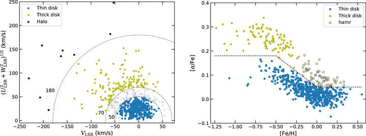
Figure 1. Decomposition of the Galactic components. Left panel: Toomre diagram of space-velocity components relative to LSR. Dashed lines show constant values of the total Galactic velocity  50, 70, and 180 km s−1. The gray region bounded by Vtot values 50 and 70 km s−1 is the neutral region characterized as a thin and thick disk star overlap probability zone. Right panel: [α/Fe]–[Fe/H] plane of our sample. The dotted line corresponds to the separation criteria of thin and thick disk components proposed by Adibekyan et al. (2013), where at [Fe/H] > − 0.2 dex in the thick disk branch, we have the defined hαmr subgroup. Stars between diagrams with the same colors do not necessarily represent the same stars.
Download figure:
Standard image High-resolution imageAnother way to separate these components is based on their chemical composition. The relative abundance ratio of chemical elements holds key information about birthplace and Galaxy formation itself. In particular, the ratio of alpha elements to iron or α-elements enhancement, [α/Fe], may indicate how quickly a star has formed and the type of supernovae that enriched its surrounding gas. Because of the observed bimodal distribution of stars in the α-element abundances as a function of metallicity, the [α/Fe] versus [Fe/H] plane is frequently used to separate the (chemical) thin- and thick-disk populations in several spectroscopic surveys (e.g., Recio-Blanco et al. 2014; Hayden et al. 2015; Queiroz et al. 2023).
Following the definition of Adibekyan et al. (2013), the identification of thin/thick disk components and hαmr stars is shown in Figure 1, from the [α/Fe]–[Fe/H] plane on the right panel. Although a small number of halo stars have been identified kinematically in the [α/Fe] versus [Fe/H] plane, we have included these stars in the conventional thin (low-α) and thick (high-α) disk chemical populations. We define the [α/Fe] abundance ratios as an average of the abundance of Si, Mg, Ti i, and Ti ii or in a similar way:

The high-α metal-rich (hereafter hαmr) stars put forward by Adibekyan et al. (2011) are a subgroup of the thick disk population defined at [Fe/H] > − 0.2 dex. They were also observed in different spectroscopic studies (Guiglion et al. 2019; Lagarde et al. 2021; Zhang et al. 2021; Queiroz et al. 2023), which suggests that stars represent the metal-rich tail of the thick disk or have an origin in the inner Galaxy (bulge) and have radially migrated up to the solar neighborhood (Adibekyan et al. 2013; Anders et al. 2018; Zhang et al. 2021).
3. The Sample
Our work sample comprises 715 dwarf stars obtained by cross-matching the HARPS-GTO Program data provided by Adibekyan et al. (2012) with the GCS (Nordström et al. 2004; Holmberg et al. 2007, 2009). The work by Adibekyan et al. consists of 1111 nearby stars (most located at distances < 90 pc from the Sun) of F, G, and K spectral types, where the majority are G-type stars, with high-resolution spectra of R ∼ 110,000 observed with the HARPS spectrograph, providing chemical abundance measurements for 12 elements (Na, Mg, Al, Si, Ca, Ti, Cr, Ni, Co, Sc, Mn, and V). Typical uncertainties in [α/Fe] ratio (α element abundance refers to the mean of Mg, Si, and Ti) and metallicity are around 0.03 dex. The HARPS sample was initially designed for the detection of planets through radial velocity measurements and was selected in such a way as to avoid biases related to metallicity. The GCS catalog is a kinematically unbiased and magnitude-limited survey that contains projected rotational velocity  measurements for about 13,000 FG(K) dwarf stars carried out by Nordström et al. (2004) and rediscussed by Holmberg et al. (2007, 2009). The
  data were computed from observations carried out with the CORAVEL photoelectric cross-correlation spectrometers, with calibrations of Benz & Mayor (1981, 1984). The resolution CORAVEL mask is optimized for stars not rotating too rapidly, presenting high-precision
  measurements even for slow rotators down to 2 km s−1, with a typical uncertainty of 1 km s−1 for stars with rotations less than 30 km s−1 (Benz & Mayor 1981, 1984). Our final working sample consists of 715 main sequence field stars with rotational velocities of up to 10 km s−1 and a precision better than about 1 km s−1.
4. Distribution Models
We examine the relationships between the projected rotational velocity distributions,  , for stars in the thin disk and thick disk components of the Galaxy. Halo populations were not considered in the analysis because of the small number of stars in this group. For this, we use the generalization of conventional statistical mechanics presented by Tsallis (1988, 2009). We recall that Tsallis formalism is a nonextensive generalization of Boltzmann–Gibbs statistics based on the entropic index q, where q is a quantity that expresses the degree of nonextensivity of the system. Here, q ≠ 1 corresponds to the non-Gaussian regime, while q → 1 recovers standard Boltzmann–Gibbs entropy.
The cumulative distribution function (CDF) for  for the two investigated galactic components can be found from a model of the type q-Gaussian (Silva et al. 2020). Considering the
  and
and ![${\exp }_{q}(x)={[1+(1-q)x]}^{\tfrac{1}{1-q}}$](https://content.cld.iop.org/journals/0004-637X/958/1/32/revision1/apjacfc3fieqn12.gif) generalizations from Tsallis's statistic, we can write q-Gaussian model as
generalizations from Tsallis's statistic, we can write q-Gaussian model as
where qg and σq are adjustable constants.
Still, within the generalized statistical space proposed by Tsallis, we will use the q-Weibull cumulative probability distribution, which contains an extra parameter for free adjustment and, theoretically, can provide us with a better fit to the data. Mathematically it can be obtained by
where qw , σw , and r are adjustable constants. When qw , r → 1 simultaneously, we recover the exponential pattern. Note that when r → 2 we return the q-Gaussian function again. A more in-depth discussion on this topic can be found in Picoli et al. (2009). Physicists employ this model in a wide variety of fields (de Freitas et al. 2019; De Assis et al. 2020; Correia et al. 2022).
5. Bayesian Inference
Before delving into a more comprehensive discussion regarding the rotations of the studied objects, it is essential to determine which of the two generalized models is more suitable. To accomplish this, we will employ Bayes's theorem, a robust statistical decision-making tool that can be expressed mathematically as follows:

Bayes's theorem gives us the probability P(Θ∣D, Φ) that a model Φ will be able to explain the data D by taking previous information about the model's adjustment parameters into account (Θ). The likelihood function  is multiplied by the probability of the model a priori P(Θ∣Φ), given the universe of possible parameters, and divided by the Bayesian evidence
  ,
,

The aim is to find the function that best matches the data by identifying the model with the most evidence within specified limits. For this, we assume that the likelihood function has the formula  , with
  , where P(lobs) and P(lthe) represent the cumulative probability for the observed and theoretical
  , respectively.
Previous information on the fit parameters was calculated with the R code using the nlsLM function (Moré 2006) with the aid of the bootstrap technique (Huet et al. 2004). The MULTINEST approach is used to obtain the  evidence with a corresponding error estimate (Feroz et al. 2009, 2013; Buchner et al. 2014). We display the evidence according to each investigated model in Table 3.
The Bayes factor, which calculates the ratio between the evidence for the models we wish to evaluate, is used to compare the evidence. Taking the natural logarithm, it can be described as

where  is the evidence of the base model, which is used as a reference, and
  is the evidence of the model we want to compare. The evidence we find will more accurately reflect the curve that best fits the data as we define more precisely the behavior of the parameters (van de Schoot et al. 2021). We employ Jeffreys's interpretation of the Bayes factor, presented in Table 1 (Jeffreys 1998) in summary form.
Table 1. The Jeffreys (1998) Scale for Interpretation of the Bayes Factor

| Interpretation |
|---|---|
| <1 | Inconclusive |
| 1 | Weak |
| 2.5 | Moderate |
| 5 | Strong |
Download table as: ASCIITypeset image
The first column of Table 1 presents the module of the Bayes factor, while the second column provides the corresponding interpretation for each interval. It is important to observe that the difference,  , can yield either a positive or a negative value. The sign will indicate which of the models presents favorable evidence. A positive value of
  favors model i, whereas a negative value suggests that model j should be prioritized.
6. Results and Discussion
In our sample, the  values span the range of 0–10 km s−1, comprising solely integer values. Accordingly, we systematically structured our data set to optimize the acquisition of the maximal number of data points, employing a bin of 1 km s−1 in the observed CDFs. In order to find better evidence and mitigate potential bias, we prioritize the largest possible number of points in the distribution. This allows for a more accurate measure of the relative merits of each model investigated, and thus enables a more informed decision-making process.
In Figure 2 we have information about the cumulative probability distributions  for the thin/thick disk and hαmr stars. The cumulative probability distributions are fitted from the theoretical curves associated with q-Gaussian (Equation (3)) and q-Weibull (Equation (4)). We can see that the Galactic components' rotational distributions between kinematic and chemical criteria are quite similar. Through the Anderson–Darling test, the chemical and kinematic thin disk are the same population with a p-value ≫ 0.25; likewise, the thick disk stars defined in the two criteria are also drawn from the same stellar population.
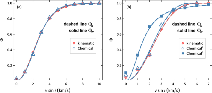
Figure 2. In (a) and (b), we have the  cumulative probability distributions of the thin and thick disk stars obtained by the kinematic and chemical methods, respectively. From the data discretization, we defined a bin width of 1 km s−1 for the observed CDFs. The best-fit curves for the theoretical Equations (3) and (4) distributions, respectively, are represented by dashed and solid curves. Index 1 indicates "genuine" thick disk ([Fe/H] < −0.2 dex) and 2 indicates hαmr subgroup (defined in [Fe/H] > −0.2 dex).
Download figure:
Standard image High-resolution imageIn contrast, while the kinematically defined thick and thin disk components show little difference (p-value = 0.15), the chemical disk components exhibit significantly different rotational distributions from each other (p-values < 0.05). Interestingly, although these differences can be attributed to the ages of each stellar group, where the thin disk stars are mostly young with a mean age ∼5 Gyr, the thick disk and hαrm populations have basically the same mean age at around 8 Gyr according to Adibekyan et al. (2011) through ages determined using the set of BASTI isochrones (see also Anders et al. 2018; Lagarde et al. 2021).
Table 2 presents the best-suited parameters for each model. Now in the context of Galactic population components, with the caveat of chemically defined thin disk stars, it becomes evident that under the q-Gaussian model, the  distributions in fact do not obey standard Gaussian or Maxwellian functions, given that
  for a 95% confidence interval. In contrast, taking into account the uncertainties associated with the entropic parameter q within a 2σ level, the q-Weibull distribution function may exhibit a standard Gaussian behavior (q = 1). Regardless of the uncertainties, the values of the best-fit parameters q and σ of the two function models are very close.
Table 2. Information on Theoretical Model Fit
| Methods | N | q-Gaussian | q-Weibull | |||
|---|---|---|---|---|---|---|
| qg | σg | qw | r | σw | ||
| Thin Disk | ||||||
| Kinematic | 432 | 1.16 ± 0.10 | 2.65 ± 0.10 | 1.14 ± 0.10 | 1.98 ± 0.10 | 2.69 ± 0.10 |
| Chemical | 555 | 1.08 ± 0.10 | 2.87 ± 0.10 | 1.09 ± 0.10 | 2.02 ± 0.10 | 2.85 ± 0.20 |
| Thick Disk | ||||||
| Kinematic | 146 | 0.82 ± 0.10 | 3.30 ± 0.20 | 0.88 ± 0.20 | 2.08 ± 0.20 | 3.17 ± 0.40 |
| Chemical1 | 93 | 0.78 ± 0.10 | 3.21 ± 0.30 | 0.84 ± 0.30 | 2.13 ± 0.40 | 3.09 ± 0.60 |
| Chemical2 | 66 | 1.44 ± 0.10 | 1.09 ± 0.10 | 1.40 ± 0.30 | 2.00 ± 0.10 | 1.23 ± 0.40 |
Note. In the first and second columns, we have the selection method and the corresponding number of objects, respectively. The subsequent columns provide the mean values of the best-fit parameters for each of the databases and their respective errors. The subscripts show that the studied distribution models qg and σg come from Equation (3), and qw , r, and σw come from Equation (4). Indexes 1 and 2 indicate "genuine" thick disk and hαmr subgroup, respectively.
Download table as: ASCIITypeset image
We investigate which of the functions best fits the data. Visually, the two studied models fit very well, so for this task, a robust and well-known selection method, Bayesian inference, was used. For more details, see Section 5.
Table 3 shows the natural logarithms of the Bayesian evidence ( ) for each model according to the selection method. Now, we can simply consider the difference between the models' evidence (see the last column of Table 3). We used the interpretation in Jeffreys (1998) for
  , similarly to what was done in da Silva & Silva (2021), and when analyzing the proposed distributions, we were unable to find a significant value, regardless of the model we take as a reference.
Table 3. The Following Are Bayesian Evidence Values for Thick/Thin Disk Stars
| Methods | q-Gaussian | q-Weibull | Bayes Factor |
|---|---|---|---|

|

|

| |
| Thin Disk | |||
| Kinematic | −3.90 ± 0.1 | −3.86 ± 0.1 | −0.04 ± 0.2 |
| Chemical | −4.40 ± 0.1 | −3.78 ± 0.1 | −0.62 ± 0.2 |
| Thick Disk | |||
| Kinematic | −0.78 ± 0.1 | −0.96 ± 0.1 | 0.18 ± 0.2 |
| Chemical1 | −0.87 ± 0.1 | −0.74 ± 0.1 | −0.13 ± 0.2 |
| Chemical2 | −2.99 ± 0.1 | −2.32 ± 0.1 | −0.67 ± 0.2 |
Note. The first column defines the method used to construct the sample, while the second and third provide evidence based on the examined model. The q-Gaussian and q-Weibull models are represented by the subscripts i and j, respectively. In the final column, the Bayes factor is shown. Indexes 1 and 2 indicate thick disk and hαmr stars, respectively.
Download table as: ASCIITypeset image
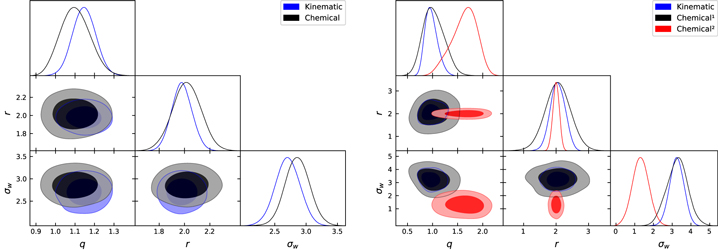
However, this is easily understood by examining Expressions (3) and (4). Function (4) is a mathematical generalization of Equation (3), so that in the limit r → 2, we return to the q-Gaussian pattern. If we look at the best-fit values in Table 2 and Figure 3, we can see that the average values for the parameter r of the q-Weibull type distribution function revolve around 2, approximating this function to q-Gaussian behavior. In this scenario, the distribution Function (3) is the best choice because it is simpler and has one fewer free parameter, thus fewer related errors. In the q-Gaussian regime, the mean values of the entropic parameter q of the thin/thick disk populations and hαmr stars are, respectively, q = 1.12, q = 0.8, and q = 1.44. It is important to note that for the chemically disentangled thin disk population, due to the boundary set by the uncertainties of the entropy index value, q = 1.08 ± 0.1, the  distributions might manifest standard Boltzmann–Gibbs entropy (q = 1). By the kinematic method of decomposition, on the other hand, the Tsallis non-Gaussian statistic is the most appropriate law to fit the distribution of projected rotational velocities of these thin disk stars.
Figure 3. Scattering of the best-fit parameters for the q-Weibull (Equation (4)) distribution, for thin (left panel) and thick disk stars and hαmr stars (right panel). Graph obtained from Bayesian inference. Indexes 1 and 2 indicate thick disk and hαmr subgroup, respectively.
Download figure:
Standard image High-resolution image
Although hαmr stars are approximately the same age as the thick disk population, the hαmr group has a subextensivity (q = 1.44). If the index q is a measure of how much angular momentum is conserved in the system, this may indicate that high-α metal-rich stars of the chemical thick disk branch of [α/Fe]–[Fe/H] plane retain part of the memory of their original angular momentum, although they are mostly old (∼8 Gyr). Consequently, it is plausible that the young star tail from this group may have higher velocities when compared to young stars from other populations.
The other possible explanation should be the long-range interactions associated with their birthplace, for instance, a strong interaction between the components of the system and the Galactic environment where the star was formed. The hαmr stars are slow rotators, but with a longer tail to high velocities, exhibiting a completely distinct distribution of rotational velocities. This indicates that the chemical thick disk stars defined at [Fe/H] < − 0.2 dex and the hαmr subgroup defined at [Fe/H] > − 0.2 dex are, in fact, distinct objects. It is worth mentioning that applying the same metallicity division to thin disk stars does not reveal any differences in their rotational velocity distributions.
As it is known, the stellar populations of the Galactic disk were probably formed in distinct phases (in time and space) and, according to Adibekyan et al. (2013) and Zhang et al. (2021), hαmr stars may have originated from the inner Galaxy (e.g., <2 kpc) and migrated to the solar neighborhood (∼8 kpc). Thus, specific regions of the Galaxy, especially the inner disk region, may be associated with particular physical processes that directly impact the initial angular momentum of stars in differing ways.
7. Conclusions
In this work, based on Tsallis's nonextensive theory, we have analyzed the observed distributions of projected rotational velocity of the Galaxy disk components and their relationships with the entropic index q.
Our results demonstrate that the q-Gaussian distribution function provides a more accurate representation of stellar rotation distributions in the chemical/kinematic thin and thick disk populations. In addition, we found that there is an anticorrelation between q and the age of the Galaxy's disk components, which supports the interpretation that the index q can be a measure of the memory of the initial angular momentum of the stellar system (Silva et al. 2013). Thus, thick disk stars experience a significant loss of angular momentum in comparison to thin disk stars.
For the old hαmr (high-α elements metal-rich) stars, we found a subextensivity with q = 1.44. Since the parameter q is also a measure of long-range interactions, in addition to its unusual prolonged subextensive regime and peculiar  distribution, we infer that these specific features of hαmr group may be linked to their place of origin in the inner region of the disk. In this way, the rotational velocities of stars are not only defined by evolutionary spin-down or random processes but also depend on their astrophysical birth sites. This is the first strong indication of a break in the isotropy of stellar rotation on global scales. Furthermore, the kinematic and chemical disk components share very similar
  properties, and our findings provide further evidence that the thick disk and hαmr groups are totally distinct populations.
Acknowledgments
M.P.d.S. is supported by CAPES through grant No. 88882.375868/2019-01. M.M.F.d.L. is supported by CAPES through grant No. 88887.609148/2021-00. J.D.N.Jr. acknowledges the financial support by CNPq funding through the grant PQ 310847/2019-2.