


Abstract
We analyze the cool gas in and around 14 nearby galaxies (at z < 0.1) mapped with the Sloan Digital Sky Survey IV MaNGA survey by measuring absorption lines produced by gas in spectra of background quasars/active galactic nuclei at impact parameters of 0–25 effective radii from the galactic centers. Using Hubble Space Telescope/Cosmic Origins Spectrograph, we detect absorption at the galactic redshift and measure or constrain column densities of neutral (H i, N i, O i, and Ar i), low-ionization (Si ii, S ii, C ii, N ii, and Fe ii), and high-ionization (Si iii, Fe iii, N v, and O vi) species for 11 galaxies. We derive the ionization parameter and ionization-corrected metallicity using cloudy photoionization models. The H i column density ranges from ∼1013 to ∼1020 cm−2 and decreases with impact parameter for r ≳ Re. Galaxies with higher stellar mass have weaker H i absorption. Comparing absorption velocities with MaNGA radial velocity maps of ionized gas line emissions in galactic disks, we find that the neutral gas seen in absorption corotates with the disk out to ∼10 Re. Sight lines with lower elevation angles show lower metallicities, consistent with the metallicity gradient in the disk derived from MaNGA maps. Higher-elevation angle sight lines show higher ionization, lower H i column density, supersolar metallicity, and velocities consistent with the direction of galactic outflow. Our data offer the first detailed comparisons of circumgalactic medium (CGM) properties (kinematics and metallicity) with extrapolations of detailed galaxy maps from integral field spectroscopy; similar studies for larger samples are needed to more fully understand how galaxies interact with their CGM.
Export citation and abstract BibTeX RIS

Original content from this work may be used under the terms of the Creative Commons Attribution 4.0 licence. Any further distribution of this work must maintain attribution to the author(s) and the title of the work, journal citation and DOI.
1. Introduction
Galaxies interact with their surroundings through gas flows. Inflows of cool gas bring in fresh material for star formation. Outflows of enriched gas carry the chemical elements produced by star formation back into the intergalactic medium (IGM). These gas flows pass through the circumgalactic medium (CGM) that acts as an interface between the galaxy and the IGM. Many aspects of the physical interactions between galaxies and the IGM are not well understood. Examples include how galaxies acquire their gas, what processes affect the chemical abundances of stars and gas, and how processes such as accretion, mergers, and secular evolution affect the growth of galaxy components.
Constraining these physical processes observationally requires spatially resolved information about the kinematics and chemical composition within and around galaxies and CGM. Integral field spectroscopy (IFS) enables spatially resolved measurements of emission-line fluxes and line ratios, allowing for construction of maps of important physical properties and their gradients such as gas kinematics, ionization, metallicity, and star formation rate (SFR). Comparisons of these rich data sets with predictions of galaxy structure and evolution models can then shed light on how disks and bulges assemble and how baryonic components of galaxies interact with their dark matter halos. A number of interesting studies using IFS have been carried out at intermediate and high redshifts to investigate the gas flows passing through the CGM (e.g., Bouché et al. 2007; Péroux et al. 2011, 2016, 2019, 2022; Fumagalli et al. 2016; Schroetter et al. 2016, 2019; Lofthouse et al. 2020, 2023). Many of these studies were based on absorption-selected samples. However, connecting these studies to local galaxies requires a parallel study of low-redshift, galaxy-selected samples.
The Mapping Nearby Galaxies at Apache Point Observatory (MaNGA; Bundy et al. 2015) survey of the Sloan Digital Sky Survey IV (SDSS IV; Blanton et al. 2017) is particularly useful in this context. MaNGA has obtained IFS data for 10,000 nearby (0.01 < z < 0.15) galaxies with 19–127 fibers, spanning 3600–10300 Å with a resolution of ∼2000. This survey has led to a number of interesting results relevant to the CGM. For example, extraplanar ionized gas with a variety of emission lines has been detected in edge-on or highly inclined MaNGA galaxies out to ∼4–9 kpc (e.g., Bizyaev et al. 2017; Jones & Nair 2019). In a significant fraction of MaNGA galaxies, this gas appears to lag in rotation compared to the gas closer to the galactic plane (Bizyaev et al. 2017).
While the MaNGA survey provides information about the structure and kinematics of the disk and bulge components in the inner 1.5−2.5 effective radii of the galaxies, it does not offer much insight about the gaseous halos of these galaxies. The H i-MaNGA program is obtaining 21 cm observations for a large fraction of MaNGA galaxies (e.g., Masters et al. 2019; Stark et al. 2021). However, this 21 cm emission survey is sensitive to relatively high H i column densities (≥1019.8 cm−2), 10 making it difficult to access the lower column-density outskirts of galaxies and the CGM.
A powerful technique to probe the gaseous galaxy halos and the CGM is by means of the absorption signatures from the gas against the light of background sources such as quasars or gamma-ray bursts. Indeed, halo/CGM gas has been detected extending to ≳200 kpc around individual galaxies (e.g., Tumlinson et al. 2013) and in large samples of stacked spectra out to ∼10 Mpc (e.g., Pérez-Ràfols et al. 2015). Probing the outskirts of MaNGA galaxies with this absorption-line technique provide a mean to establish a local sample of exquisitely imaged galaxies studied in neutral and ionized gas. Such a local sample is essential for placing IFS observations of high-redshift galaxies and their CGM in perspective, and thereby developing a systematic understanding of the interactions between galaxies and the gas flows around them, and the evolution of these interactions with time.
With these improvements in mind, we have started to investigate the interstellar medium (ISM) and CGM of MaNGA galaxies using the Hubble Space Telescope (HST) Cosmic Origins Spectrograph (COS). Here we describe the results from our COS observations of 14 MaNGA galaxies, and compare the gas properties deduced from the COS data to the properties of the ionized gas measured from the MaNGA data.
This paper is organized as follows. Section 2 describes the sample selection, observations, and data reduction. Section 3 describes results from our COS spectroscopy. Section 4 presents a discussion of our results, including comparisons with the MaNGA data and other studies from the literature. Section 5 presents our conclusions. Throughout this paper, we adopt the "concordance" cosmological parameters (Ωm = 0.3, ΩΛ = 0.7, and H0 = 70 km s−1 Mpc−1).
2. Observations and Data Reduction
2.1. Sample Selection
Our sample consists of 14 nearby galaxies (at z < 0.1) mapped in the SDSS/MaNGA survey with UV-bright quasars/active galactic nuclei (AGNs) at impact parameters between 0 and 140 kpc from the galactic centers. The targeted quasars have GALEX FUV mag < 19.5, and their impact parameters range from 0–25 times the effective radii of the corresponding MaNGA galaxies. For 1-635629, a bonus galaxy covered in the same setting as 1-180522, the impact parameter is 38.7 Re .
We performed HST COS spectroscopy for these quasars/AGNs, as described in Section 2.2. The targets are listed in Table 1. We divide the targets into two groups by the value of impact parameter. The first group contains four objects with zero impact parameter, because in these cases we observed the central source, hereafter referred to as AGNs (see Figure 1). In these cases, the absorbing gas can be at any distance from the central source along the line of sight, and could potentially be associated with the central engine. Physical conditions in the absorbing gas in such cases can be very different from those in the CGM and ISM. The objects in the second group have nonzero impact parameters (more than 20 kpc) and likely probe gas related to the CGM of the galaxies (see Figure 2). In two cases (J2130−0025 and J0838+2453), the quasar sight lines cross two galaxies at different impact parameters and redshifts.
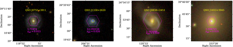
Figure 1. The images of four galaxies with zero impact parameter. Each panel shows the SDSS three-color image of the area near the MaNGA galaxy. The image is centered at the position of the galaxy. The pink hexagons show the sky coverage of the MaNGA IFU. The yellow circles show the position of the HST/COS aperture centered on the galactic nucleus.
Download figure:
Standard image High-resolution image
Figure 2. Images of galaxy–quasar pairs with nonzero impact parameters. The panels are arranged in order of increasing impact parameter. Each panel shows the SDSS three-color image of the area near the MaNGA galaxy. The image is centered at the position between the quasar and the galaxy. The pink hexagon shows the sky coverage of the MaNGA IFU. The yellow circle represents the position of the quasar and has the size of the HST/COS aperture. The distance between the quasar and the center of the MaNGA galaxy at the galaxy redshift (the impact parameter) is shown by the pink link.
Download figure:
Standard image High-resolution imageTable 1. Physical Properties of the Sample of MaNGA Galaxies and Background Quasars
| MaNGA | zgal |

| SFR | log sSFR | Dn (4000) a | Quasar | zquasar | Imp Par. | Re | b/Re |
|---|---|---|---|---|---|---|---|---|---|---|
| ID | (M⊙) | (M⊙ yr−1) | (yr−1) | (b) (kpc) | (kpc) | |||||
| 1-71974 | 0.03316 | 10.30 | 1.72 | −10.06 | 1.30 | J0755+3911 | 0.0332 | 0 | 4.9 | 0 |
| 1-385099 b | 0.02866 | 10.69 | 0.20 | −11.38 | 1.54 | J0838+2453 | 0.0287 | 0 | 5.4 | 0 |
| 12-192116 | 0.02615 | 8.80 | 0.59 | −9.03 | 1.22 | J1338+2620 | 0.0261 | 0 | 3.3 | 0 |
| 1-594755 | 0.03493 | 10.78 | N/A | N/A | 1.23 | J1653+3945 | 0.0349 | 0 | 1.3 | 0 |
| 1-575668 | 0.06018 | 11.02 | N/A | N/A | 1.87 | J1237+4447 | 0.4612 | 39 | 10.6 | 3.8 |
| 1-166736 | 0.01708 | 8.98 | 0.08 | −10.07 | 1.31 | J0950+4309 | 0.3622 | 23 | 3.4 | 6.9 |
| 1-180522 b | 0.02014 | 9.31 | 0.55 | −9.56 | 1.26 | J2130−0025 | 0.4901 | 34 | 4.1 | 8.5 |
| 1-561034 | 0.09008 | 10.86 | N/A | N/A | 1.86 | J1709+3421 | 0.3143 | 75 | 6.0 | 12.8 |
| 1-585207 b | 0.02825 | 10.09 | N/A | N/A | 1.93 | J0838+2453 | 0.0287 | 37 | 2.4 | 15.5 |
| 1-113242 | 0.04372 | 10.88 | N/A | N/A | 2.14 | J2106+0909 | 0.3896 | 116 | 5.5 | 22.9 |
| 1-44487 b , c | 0.03157 | 10.47 | 1.34 | −10.34 | 1.74 | J0758+4219 | 0.2111 | 136 | 6.2 | 22.6 |
| 1-44487 b , c | 0.03174 | N/A | N/A | N/A | N/A | J0758+4219 | 0.2111 | 137 | N/A | N/A |
| 1-564490 | 0.02588 | 10.15 | 2.60 | −9.73 | 1.27 | J1629+4007 | 0.2725 | 132 | 5.7 | 23.8 |
| 1-635629 c | 0.01989 | 9.56 | 1.26 | −9.45 | 1.34 | J2130−0025 | 0.4901 | 66 | 1.7 | 38.7 |
Notes.
a The 4000 Å break (Dn (4000)) was measured between 1 < R/Re < 1.5 to avoid the AGN contamination. b Quasar–galaxy pairs have the same quasar sight lines. c The case of merged galaxies. N/A—not applicable, or not available.Download table as: ASCIITypeset image
2.2. HST/COS Data
Our sample of 11 quasars was observed with HST COS under program ID 16242 (PI V. Kulkarni) during 2020 September–December. These observations are summarized in Table 2. The FUV channel of COS was used in TIME-TAG mode. The G130M FUV grating and the 2 5 Primary Science Aperture were used. The grating was centered at 1222 and 1291 Å to cover the absorption lines of interest. This leads to a resolving power across the dispersion axis of R ∼ 10,000–18,000. The grating settings were optimized so that the key lines do not fall in the gaps in the wavelength coverage or in geocoronal emission lines. Target acquisitions were performed using the ACQ/IMAGE modes, after which 3–11 exposures ranging from 515–1339 s each were obtained for each target.
Table 2. HST COS Observing log
| Quasar | zquasar | R.A. | Decl. | Date | COS Setting |
 a
a
| S/N b |
|---|---|---|---|---|---|---|---|
| (J2000.0) | (J2000.0) | (s) | |||||
| J0755+0311 | 0.0332 | 118.85 | 39.18 | 2020 Sep 11 | G130M/1291 | 2192 | 13.5 |
| J0758+4219 | 0.2111 | 119.58 | 42.32 | 2020 Sep 6 | G130M/1222 | 2147 | 5.3 |
| J0838+2453 | 0.0287 | 129.55 | 24.89 | 2020 Oct 29 | G130M/1222 | 7436 | 7.4 |
| J0950+4309 | 0.3622 | 147.56 | 43.15 | 2020 Nov 27 | G130M/1222 | 15254 | 9.4 |
| J1237+4447 | 0.4612 | 189.39 | 44.79 | 2020 Dec 16 | G130M/1222 | 4986 | 9.9 |
| J1338+2620 | 0.0261 | 204.51 | 26.34 | 2020 Dec 17 | G130M/1222 | 2062 | 4.5 |
| J1629+4007 | 0.2725 | 247.26 | 40.13 | 2020 Sep 2 | G130M/1222 | 7631 | 10.4 |
| J1653+3945 | 0.0349 | 253.47 | 39.76 | 2020 Oct 8 | G130M/1222 | 2086 | 13.7 |
| J1709+3421 | 0.3143 | 257.49 | 34.36 | 2020 Sep 3 | G130M/1291 | 9592 | 12.0 |
| J2106+0909 | 0.3896 | 316.71 | 9.16 | 2020 Oct 10 | G130M/1222 | 7376 | 4.5 |
| J2130−0025 | 0.4901 | 322.59 | −0.43 | 2020 Sep 12 | G130M/1222 | 19310 | 7.8 |
Notes.
a The total integration time (summed over all exposures). b The signal-to-noise ratio (S/N) was calculated at 6 pixel binning at ≃1250 Å.Download table as: ASCIITypeset image
For a majority of the targeted galaxies, we clearly detect strong absorption lines of H i, Si ii, and Si iii at redshifts close to the galactic redshifts (within ±200 km s−1). Since there are no other galaxies at these redshifts around the quasar sight lines (within ∣zphotom − zgal∣ < 0.05 and ∼100 kpc and down to SDSS magnitude r ≃ 22), our HST COS spectra probe the CGM of the selected MaNGA galaxies. 11 The profile fits to the HST COS absorption line data and the measurements of column densities are presented in detail in Appendix B.
2.2.1. Data Reduction and Spectral Extraction
The original CalCOS pipeline v3.4.0 was first used to reduce the HST COS exposures and extract the 1D spectra. However, a reanalysis of the data was found to be necessary, because some of our exposures had low counts (Ncounts ≃ 1–10 pix−1). For these exposures, the flux uncertainties in individual exposures were found to be overestimated using the original pipeline. The flux variance was ∼2 times lower than the flux uncertainties estimated by the standard pipeline, and the difference was found to be correlated with the flux value. The procedure for estimating the flux uncertainty in the original pipeline was therefore modified in our reanalysis of the data.
This problem was described in the ISR COS 2021-03 (Johnson et al. 2021), where it is shown that the number of received counts is described by a binomial distribution with an asymmetric shape at low count levels (N ≤ 10). The CalCOS pipeline uses the method developed by Gehrels (1986) to estimate flux uncertainties in this case. However, we found that the 1σ uncertainties derived by Gehrels (1986) correspond to 63.8% quantile interval, which is shifted to positive values relative to the uncertainties derived with the maximum likelihood estimate. This shift slightly reduces the negative uncertainty and increases the positive uncertainty. In spectra corrected for this shift, the 1σ uncertainties correspond well to the flux dispersion values. Therefore, flux errors were reevaluated based on the modified estimates. Further details are provided in Appendix A.
The procedure for the subtraction of the noise background also does not work well in a low-count regime, and was therefore also modified. Originally, for each exposure the average background flux was calculated from the detector area free from the science target and wavelength calibration lamp signals. This average background flux was subtracted from the science spectrum in each exposure. However, in cases of low flux levels, the number of noise counts is also very low (e.g., 1–2 counts per 10 pixels); therefore, the average background flux corresponded to a fractional number of counts (about ∼0.2 counts pixel−1) and its subtraction shifted the zero-flux level to negative values, which was also observed in the final spectrum of the coadded exposures in the cores of saturated absorption lines. Therefore, instead of using this method for background subtraction, we used the following approach: we derived the background flux from the final spectrum of coadded "background" exposures, which were extracted by the same method as that used for the extraction of the science exposures, but the method was applied to a shifted extraction box in the detector area free from the science target and wavelength calibration lamp signals (and with a minimum content of bad-quality pixels, including the gain sag hole and poorly calibrated regions). The "background" exposures were next coadded, rebinned, smoothed by 10 pixels and then subtracted from the science exposure. This approach allows for a more accurate estimate of the average background flux level (since it gives a number of noise counts per bin strongly exceeding 1) and enables the calculation of the wavelength dependence of the background.
2.2.2. Spectral Analysis
For each quasar/AGN, we analyzed the absorption systems at the redshifts of associated MaNGA galaxies. Figure 3 shows examples of our analysis for the four galaxies shown in Figure 2. Fits for the remaining sight lines are shown in Appendix B. To perform this analysis, we used a custom modification of the Voigt profile fitting code 12 to derive the redshifts, column densities, and Doppler parameters of velocity components for H i, N i, O i, Ar i, and various low-ionization (Si ii, S ii, C ii, N ii, and Fe ii) and high-ionization (Si iii, Fe iii, N v, and O vi) metal absorption lines. The wavelengths and oscillator strengths for these transition were taken from Morton (2003). Further details about this code and examples of its usage can be found in Balashev et al. (2017, 2019).
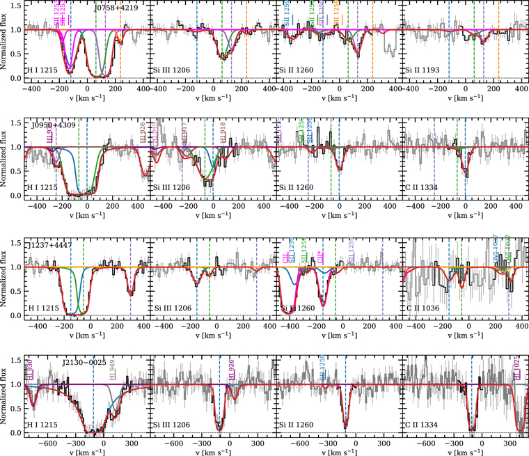
Figure 3. The absorption lines of H i, Si iii, Si ii, and C ii in the HST COS spectra of J0758+4219, J0950+4309, J1237+4447, and J2130−0025 at the redshifts of the corresponding galaxies (1-44487, 1-166736, 1-575668, and 1-180522, respectively). The synthetic profile is shown in red, and the contribution from each component, associated with the studied galaxy, is shown in green, blue, purple, and orange. The dashed vertical lines represent the position of each component. Vertical ticks indicate the position of absorption lines, associated with the Milky Way (MW, magenta sticks) and remote galaxies.
Download figure:
Standard image High-resolution imageFor each absorption line (except the case of damped H i Lyα described below), we derived the local continuum using a B-spline interpolation matched on the adjacent unabsorbed spectral regions. The spectral pixels used to constrain the fit were selected visually. The number of velocity components was also defined visually and increased in case of remaining structure in the residuals. Since our spectra have low signal-to-noise ratio (S/N ∼1–10) and given medium spectral resolution (∼20 km s−1), we cannot resolve the velocity structure in detail. Therefore, the redshifts and Doppler parameters were tied for all species for each velocity component. The fit to each absorption lines was calculated by the convolution of the synthetic spectrum with the COS line spread function (LSF) chosen for the appropriate COS setting. 13 For weak lines, we present measurements of column densities where possible, and 3σ upper limits in cases of nondetections.
The H i column density was measured from the Voigt profile fit to the Lyα line. 14 For most of our spectra, the H i line is not damped (with N(H I) ≤ 1018 cm−2) and corresponds to the linear or flat parts of the curve of growth. In these cases, the number of components and b-values should be accurately constrained. Therefore, the number of components was defined visually from fitting to the profiles of associated metal lines (Si ii, Si iii, and C ii), and increased in case of remaining structure in the residuals. The range of b-parameters was constrained to 15–100 km s−1 (the values of b-parameters measured for H i absorbers at z ≤ 1 in the COS CGM Compendium (Lehner et al. 2018), where H i lines were fitted using several transitions in the Lyman series). Then the redshift, b-parameter, and H i and metal column densities for each component were varied together using the AffineInvariantMCMC sampler by MADS 15 to obtain the posterior probability density function (PDF) of the fitting parameters. The column density of H i and metals and the b-parameters can be rather uncertain for individual components that are blended; however, the total column densities summed over the components are usually well constrained (with uncertainty ∼0.3 dex). We demonstrate the posterior PDF of fitting parameters for systems shown in Figure 3 in Appendix B, along with comments to fits for individual systems.
For one case, the galaxy J1338+2620, the absorption Lyα line shows damping wings and is located close to the galaxy Lyα emission line. An interesting feature of this spectrum is that both the emission Lyα line and absorption Lyα line are shifted relative to their expected positions. The emission Lyα line is redshifted by 150 km s−1 with respect to the galactic redshift derived by positions of other emission lines (Hα, Hβ, S ii, N ii, and O iii) seen in the SDSS spectrum. The emission lines are very narrow ∼300 km s−1 (similar to those for type II Seyfert galaxies), which allows the redshift to be well constrained. The Lyα absorption line has a broad core (∼300 km s−1 wide), and its center is blueshifted by −150 km s−1 with respect to the strongest component of the metal absorption lines (Si ii, S ii, and O i). Additionally we detect a decrease of the local continuum near the Lyα absorption and Lyα emission lines, which is consistent with the presence of the damped Lyα (DLA) absorption line with broad damping wings and high H i column density (1020.3 cm−2). However, such an H i Lyα line is expected to have a broad bottom ∼600 km s−1, twice the observed value. We believe this situation is similar to studies of proximate DLA absorption systems in quasar spectra, which work as a natural coronagraph for the Lyα emission from the accretion disk, while the leaking Lyα emission remains partially blended in the wings of the DLA system (see, e.g., Noterdaeme et al. 2021). In this case we simultaneously fitted both the absorption profile and the unabsorbed quasar continuum.
We consider two potential ways to fit the Lyα line in this spectrum: (i) it could be a sub-DLA system that covers the Lyα emission line only partially. In this case, the local continuum was modeled as the sum of a smooth component and a Gaussian emission line. The smooth component represents the flat part of the quasar continuum and was reconstructed locally by fitting with a B-spline interpolation. The Lyα emission line was fitted by a Gaussian function centered on the redshift of the quasar. The H i Lyα absorption line was fitted by the sum of four velocity components, whose redshifts were tied to the redshifts of the velocity components in metal absorption lines (O i, Si ii, S ii, Fe ii, and Si iii). A detailed fit to metal lines is provided in Appendix B. In this case, we derive the total H i column density (1019.2±0.1 cm−2), and the best fit is shown in the top panel of Figure 4. We note, however, that (i) we needed to decrease the continuum level manually in the vicinity of the sub-DLA system, and (ii) the strongest H i component (1019.2±0.1) is shifted to −150 km s−1 relative to the strongest component in the metal absorption lines.
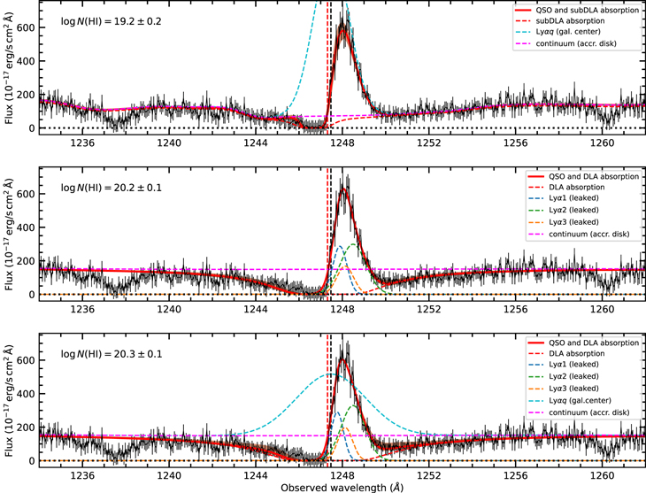
Figure 4. Fit to the H i Lyα absorption line in the spectrum of galaxy J1338+2620. Top, middle, and bottom panels shows different solutions: sub-DLA + galactic Lyα line, DLA + leaked Lyα emission, and DLA + leaked Lyα emission + galactic Lyα line, respectively (see details in the text). The black line represents the observed HST/COS spectrum, the red line shows the best fit. The red shaded area represents a variation of the synthetic fit due to the variation of H i column density within the derived uncertainty. The profile of the absorption Lyα line is shown by the red dashed curve. The smooth part of the reconstructed continuum is shown by the dashed pink curve. The cyan dashed curves in the top and bottom panels represent the reconstructed emission Lyα lines from the galactic center. The blue, orange, and green dashed lines in middle and bottom panels show the components used to fit the leaked Lyα emission. The red and black vertical lines denote the redshift of the strongest metal absorption component and the redshift of quasar, respectively. The derived total H i column density is given in the top-left corner of each panel.
Download figure:
Standard image High-resolution image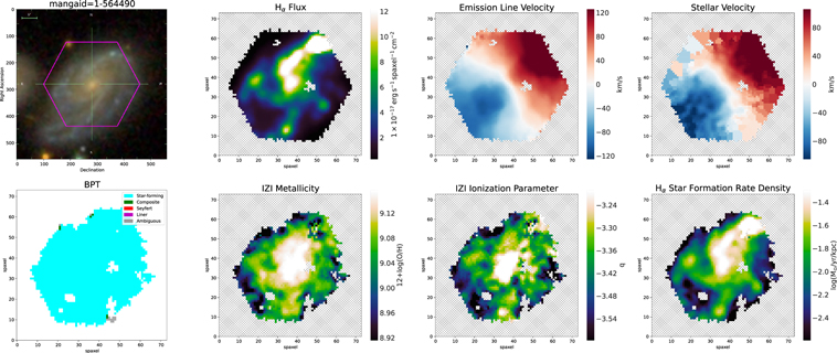
Figure 5. The physical properties of the SDSS MaNGA galaxy 1-564490. The top panels show from left to right the SDSS three-color image, the Hα line emission map, the Hα line velocity map, and the stellar velocity map. The bottom panels shows the BPT diagram and maps of IZI metallicity, IZI ionization parameter, and the density of star formation rate (SFR).
Download figure:
Standard image High-resolution imageThe second possibility is a combination of a broader, more damped Lyα absorption line and leaked Lyα emission. The damped Lyα line was centered at the redshift of the strongest metal component at z = 0.026043. The profile of the leaked Lyα emission is non-Gaussian; therefore, it was fitted by a sum of three Gaussian lines. In this case, we derive the H i column density 1020.2±0.1 cm−2. The fit is shown in the middle panel of Figure 4. The absorption Lyα line is broad (∼600 km s−1) and likely covers the emission Lyα line from the galactic center completely. In the bottom panel, we also show the fit by a model, where the galaxy Lyα emission line at the quasar redshift is added to the fit. However, the difference in the fit profile and the derived H i column density is small, compared to the fit (middle panel) without including the galaxy Lyα emission (∼0.1 dex).
The advantage of the fitting approach including the leaked Lyα emission is that (i) it can describe the decrease of the local continuum near the Lyα absorption without manual modification of the smooth B-spline fit and (ii) the redshift of H i component matches the redshift of the strongest metal components well. Therefore we adopt the column density of H i for this system to be 1020.2±0.1 cm−2.
2.3. SDSS-IV/MaNGA Data
The MaNGA (Bundy et al. 2015) survey is one of the three main components making up SDSS-IV (Blanton et al. 2017). Completed in 2020 June, MaNGA made integral field unit (IFU) spectroscopic observations of just over 10,000 galaxies using the 2.5 m Sloan Telescope at Apache Point Observatory (Gunn et al. 2006). These galaxies were selected from the extended version of the NASA-Sloan Atlas (NSA; Blanton et al. 2017; Wake et al. 2017) to be in the redshift range of 0.01 < z < 0.15 and have an approximately flat number density distribution as a function of stellar mass between 109 and 1012 M⊙. The targets were further chosen so that they could be covered by the MaNGA IFU bundles out to either a radius of 1.5 or 2.5 times the effective radius (Re ). Full details of the MaNGA sample selection are given in Wake et al. (2017).
The 17 MaNGA IFU bundles are hexagonal in shape with sizes in the range 12"–32" matched to the typical angular size distribution of the target sample of galaxies. In addition, there are 12 seven-fiber mini-bundles that are placed on flux calibration stars, and 92 single fibers for sky subtraction (Drory et al. 2015). All of the fibers feed the dual-channel Baryon Oscillation Spectroscopic Survey spectrographs (Smee et al. 2013), which cover a wavelength range of 3622–10354 Å with a median spectral resolution of ∼2000.
In this paper we use the reduced MaNGA data produced by the MaNGA Data Reduction Pipeline (Law et al. 2016) as well as derived data products produced by the MaNGA Data Analysis Pipeline (DAP; Westfall et al. 2019). These derived products include maps of various emission lines ([O ii], Hβ, [O ii], [N ii], Hα, [S ii]), and emission line and stellar velocities. We access and interact with MaNGA data using the Marvin (Cherinka et al. 2019) Python package.
We also make use of integrated galaxy properties included in the MaNGA data set that are derived from the extended version of the NSA. These include redshift, total stellar mass (M*), elliptical effective radius (Re ), and inclination, all derived from elliptical Petrosian aperture photometry (see Wake et al. 2017, for details).
2.3.1. Nebular Metallicity and Ionization Parameter
In order to connect the properties of the CGM absorption systems detected in our COS spectra with the gas within the MaNGA galaxies, we derive maps of the metallicity and ionization parameter of emission lines originating in the nebulae photoionized by massive stars.
To make these measurements, we use the Bayesian strong emission line (SEL) fitting software IZI initially presented by Blanc et al. (2015) and extended to utilize a Markov Chain Monte Carlo (MCMC), additionally fitting for extinction by Mingozzi et al. (2020). IZI compares a grid of photoionization models with a set of SELs and their uncertainties, to derive the marginalized posterior PDFs for the metallicity ( ), the ionization parameter (
 ), and the line-of-sight extinction (E(B − V)). Such an approach takes into account the covariance between these parameters, which is not insignificant.
In this work we follow the approach of Mingozzi et al. (2020), who ran IZI on a subset of the MaNGA sample. We use the photoionization model grids presented in Dopita et al. (2013) fitting for [O ii]λ3726, 3729, Hβ, [O ii]λ4959, 5007, [N ii]λ6548, 6584, Hα, [S ii]λ6717, and [S ii]λ6731. We only fit spaxels that are classified as star-forming according to either the [N ii]- or [S ii]-Baldwin, Phillips & Terlevich (BPT) diagrams (using the regions defined by Kauffmann et al. 2003 and by Kewley et al. 2001). We further restrict to spaxels with an S/N > 15, which ensures sufficient S/Ns in the remaining SELs we use. Figure 5 presents the example of MaNGA observations of the galaxy 1-544490. It shows maps of Hα flux, gas kinematics, SFR and the physical conditions derived from IZI modeling.
2.3.2. Galaxy Rotational Velocities
Beyond the ionization properties described above, we are also interested to see if there is any association between the velocity of the CGM absorption systems and galaxy rotational velocity. One might imagine the absorption systems tracing the gas dynamics at large radii.
In order to make such a connection, we fit disk rotation models to the stellar and gas velocity fields using models similar to those described in Bekiaris et al. (2016). We assume a flat thin disk in all cases linking the observed coordinates (x, y) to the projected major and minor axes coordinates of the disk (xe, ye) using:


where PA is position angle, and (x0, y0) are the coordinates of the center of the disk.
We define the radius of the disk r in the disk plane at the observed coordinates (x, y) as:
where i is the inclination of the disk to the line of sight.
The position angle relative to the major axis of the disk, θ, at (x, y) is given by

To model the rotation curve, we make use of a two-parameter arctan profile (Willick et al. 1997):

where Vrot(r) gives the rotation velocity at radius r, rt is the turnover radius, and Vt is the asymptotic circular velocity. At large radii beyond rt, this model represents a very slowly rising rotation curve.
Our final model for the velocity in the plane of the sky is given by

where Vsys represents any velocity offset from the systemic redshift used to generate the MaNGA velocity field. This model contains seven free parameters that we must fit for.
For all galaxies, we attempt to fit both the emission line and stellar velocity maps provided by the MaNGA DAP. We make use of the default MILESHC-MASTARSSP hybrid maps, which use a Voronoi binning scheme for the stellar velocities and individual spaxels for the emission-line velocities (see Westfall et al. 2019, for details). For the stellar velocity maps, we fit to all Voronoi bins that have not been masked by the DAP and have an S/N > 10. For the emission-line maps, we again exclude all masked spaxels and fit to those spaxels where any of the Hα, [O ii], or [O iii] lines have an S/N > 5. We also mask any regions of the maps not associated with the target galaxy, for instance the very close satellite galaxy of 1-44487.
We fit our model using the MCMC code emcee (Foreman-Mackey et al. 2013). We make an initial simpler fit to estimate the position angle and use that as our initial guess for that fit parameter. For the center, inclination, and rt we make initial estimates based on the NSA photometry. For Vsys, our initial estimate is the median velocity within  . Finally, we set Vt to 200 km s−1 as our initial guess for all galaxies. For each fit, use 64 walkers each with 20,000 steps, discarding the first 10,000. We fit both the emission and stellar velocity maps simultaneously and each independently, potentially giving three fits for each galaxy.
3. HST/COS Fitting Results
We detect associated absorption for 11 out of the 14 MaNGA galaxies. H i Lyα absorption is detected in all 11 of these cases, while Si ii and Si iii are detected in seven of the 11 cases. For two sight lines, each of which has two galaxies with closely spaced redshifts, we detect absorption in H i, Si ii, and Si iii (and C ii in one case), but we cannot reliably determine which galaxy corresponds to which velocity component in the detected absorption. In three cases, we do not detect any absorption (in H i or any of the metal ions) within the range of ±800 km s−1 relative to the galaxy redshifts; in these cases, we set upper limits on N(H I) ∼ 1013 cm−2. For two of these sight lines, J1709+3421 and J2106+0909, the absence of any absorption may be because of high values of the impact parameters 75 and 116 kpc, respectively (with b/Re of 12.8 and 22.9). The absence of any lines is more surprising in the third case J1653+3945, a galaxy sight line with zero impact parameter, and may be a result of high ionization of the gas. We discuss ionization corrections in Section 3.1 below.
Table 3 summarizes the results of our fits. We present the absorption redshifts, total column densities of H i, and associated strongest metal ions (Si ii, Si iii, and C ii) and results of the photoionization code simulations. We refer to the sight lines with zero impact parameters as the "galactic" sight lines and list them in the first five lines of Table 3 before the remaining sight lines that we refer to as "quasar sight lines."
Table 3. Neutral Gas and Metallicity Measurements from HST Observations
| Quasar | zabs |

|

|

|

| Si iii/Si ii | [X/H] |

|

|

| F⋆ a | |
|---|---|---|---|---|---|---|---|---|---|---|---|---|
| (cm−2) | (cm−2) | (cm−2) | (cm−2) | (cm−2) | ||||||||
| AGNs | J0755+0311 | 0.0330 |

|

|

|

|

|

|

|

|

|

|
J0838+2453
| 0.0280 |

|

|

| N/C |

|

|

|

|

|

| |
J0838+2453
| 0.0256 |

| <13.6 |

| N/C | N/A |

|

|

|

| <1 | |
| J1338+2620 | 0.0260 |

|

|

| N/C |

|

|

|

|

|

| |
| J1653+3945 | 0.0341 | <12.8 | <12.7 | <12.0 | N/C | N/A | N/A | N/A | N/A | N/A | N/A | |
| Quasars | J1237+4447
| 0.0597 |

| <13 |

| <14.7 | N/A |

|

|

|

|

|
J1237+4447
| 0.0597 |

| <13 |

|

| N/A |

|

|

|

|

| |
| J0950+4309 | 0.0170 |

|

|

|

|

|

|

|

|

|

| |
| J2130−0025 | 0.0195 |

|

|

|

|

|

|

|

|

|

| |
| J1709+3421 | 0.0880 | <13.5 | <12.5 | <13.0 | N/C | N/A | N/A | N/A | N/A | N/A | N/A | |
| J2106+0909 | 0.0442 |

| <13.0 | <13.2 | N/C | N/A | N/A | N/A | N/A | N/A | N/A | |
| J0758+4219 | 0.0320 |

|

|

| N/C |

|

|

|

|

|

| |
| J1629+4007 | 0.0240 | <13.2 | <12.5 | <12.6 | N/C | N/A | N/A | N/A | N/A | N/A | N/A | |
Notes. The first five rows (above the horizontal line) correspond to AGN sight lines with zero impact parameter, and the rest (below the horizontal line) correspond to quasar sight lines with nonzero impact parameter. Indices A,B in the first column indicate two distinct absorption systems with a high velocity separation (∼800 km s−1) in the spectrum of the AGN J0838+2453 and two different solutions for the fit to the H i profile in the spectrum of J1237+4447 (see details in Appendix B).
a F*—The parameter of the model of dust depletion by Jenkins (2009). N/C—The lines are not covered by the HST/COS spectrum. N/A—In this case, physical parameters cannot be constrained by the photoionization model.Download table as: ASCIITypeset image
The H i column density ranges from ∼1013 cm−2 to ∼1020.2 cm−2 for the AGN sight lines with H i detections and from ∼1014 cm−2 to ∼1019 cm−2 for the quasar sight lines with H i detections (i.e., with N(H I) > 1013 cm−2). For most of the systems we detect associated absorptions of low (Si ii, C ii, and N ii) and high (Si iii) ionization ions and also set upper limits on weak absorption by N i, N v, O i, and Fe ii. Detailed fits for each system are shown in Appendix B, and fit results to individual velocity components are presented in Table 5.
In Figure 6, we examine the dependence of the column densities of the strongest metal ions detected in absorption (Si ii, Si iii, and C ii) on the H i column density. There is an overall increase of Si ii, Si iii, and C ii column densities with N(H I). A similar trend was also reported previously by Lehner et al. (2018), Muzahid et al. (2018), and Werk et al. (2013) in the HST COS surveys of H i absorption systems in quasar spectra: COS CGM Compendium (at zabs < 1), COS-Weak (zabs < 0.3) and COS-Halos (zabs < 0.35), respectively. The results for our quasar sight lines are consistent with these trends. A difference is observed for the AGN sight lines: for J0838+2453 and J0755+0311, we detect higher metal column densities than those predicted by the trend for quasar absorption systems, for J1338+2620, the metal column densities are slightly lower. To demonstrate this in detail, we also show in Figure 6 theoretical constraints on the metal and H i column densities calculated under simple assumptions: N(X)/N(H I) = (X/H)⊙ ZfX/fH I, where ( X/H)⊙ is the solar abundance of element X, Z is the metallicity relative to the solar level from Asplund et al. (2009), fH I = N(H I)/N(Htot) is the H i fraction, and fX = NX/N(Xtot) is the fraction of element X in the particular ionization stage considered. For physical conditions expected in the ISM and CGM, we assume ranges of Z = 0.1–1, fH I = 10−3–10−1 and fX = 0.1–1, and vary the factor ZfX/fH I between 10−1 and 103. These constraints are fulfilled for all quasar absorption systems from our sample and from other COS surveys, while the detections and upper limits for our AGN sight lines are beyond these constraints.

Figure 6. The comparison of total column densities of Si ii, Si iii, and C ii, and the Si iii/ Si ii ratio with N(H I). Our systems are shown by diamonds (AGN sight lines) and circles (quasar sight lines). The colors of points encode the names of the systems in our sample. We also show upper limits for three nondetections: J1709+3421 (yellow circle), J1629+4007 (black circle), and J1653+3945 (purple diamond). Gray, blue, and cyan squares represent data from different COS surveys: COS-Weak (Muzahid et al. 2018), COS CGM Compendium (Lehner et al. 2018), and COS-Halos (Tumlinson et al. 2013; Werk et al. 2013), respectively. Spearman rank-order correlation coefficient rs and the p-value for our sample (all systems and only QSO absorptions) are given at the top-left corner of each panel. Black lines indicate the range of theoretical constraints on the column densities of metal ions and H i for the parameters (Z, fH I fX) typical for the ISM/CGM (see the text).
Download figure:
Standard image High-resolution imageWe also present the Spearman rank-order correlation coefficient (rS) and the probability that the observed value of rS could arise purely by chance (p-value) for all of our systems and quasars only in the top-left corner of each panel in Figure 6. The ratio N(Si III)/N(Si II) shows a statistically significant correlation (rS = 1.0 and p = 0.0) with the H i column density for our quasar sight lines (although we caution that our sample consists of only three measurements). This correlation is consistent with the correlation seen in the COS-Weak survey, which, however, had low statistical significance (rS = 0.13 and p = 0.63). For sight lines in the COS-Halos survey, there are mainly lower limits.
We also note that the samples of quasar absorption systems from the COS-Weak and COS CGM Compendium surveys were selected by a blind method (or based on availability in the HST archives), while the quasar sight lines in our sample and from the COS-Halos survey were selected to have relatively small impact parameters. The consistency of our results with those of these other studies suggests that, on average, H i absorption with N(H I) > 1015 cm−2 and associated metal features can correspond to the CGM of galaxies with impact parameters ≤∼140 kpc.
3.1. Ionization Corrections
Since our systems are not self-shielded from ionizing UV radiation, we need to calculate the ionization corrections to estimate the physical conditions and metallicity.
We used the photoionization code cloudy to infer the ionization structure of systems and estimate the metallicity, ionization parameter, and total hydrogen column density. We assumed a constant-density model in a plane parallel geometry illuminated by the radiation field and cosmic rays (CRs). The radiation field was modeled as consisting of two parts: the extragalactic UV background (UVB) radiation at z = 0.1 as computed by Khaire & Srianand (2019), 16 and the galaxy light component modeled by the interstellar radiation field as per the cloudy template, which is consistent with the Draine model in the UV range (Draine 1978). The interstellar radiation field was scaled by the factor IUV to characterize the strength of the UV radiation from the nearby galaxy. This factor is especially important for our AGN sight lines (i.e., those with zero impact parameter), for which the distance of the absorbing region from the galactic center is unknown.
The UV and X-ray radiation produced by the galaxy (by stars and the AGN) is generally ignored for the CGM absorption systems because the H i ionizing photons produced within the galaxy are assumed to be absorbed by the neutral hydrogen and dust within the galaxy. Indeed, the average escape fraction of the H i ionizing photons from galaxies is assumed to be very low (<1%) at z < 1 (see, e.g., Khaire & Srianand 2019). However, the UV spectral observations of nearby galaxies (including our AGN sight lines) do not show the strong damped Lyα absorption line associated with the neutral hydrogen in those galaxies. Moreover, the spectra usually have strong Lyα emission lines. This indicates that the H i ionizing radiation can leak out of the galaxies along these sight lines and increase the UV background around the galaxies. The intrinsic spectral energy distribution (SED) of the galactic radiation is unknown for our galaxies; therefore, we chose one of the cloudy templates to model this radiation. The SED of this interstellar radiation model is similar to that for the UVB model, and about 100 times more intense in the range of 1–100 eV at IUV = 1. Therefore, we varied this parameter in the range of  to allow for a wide range of values of the escape fraction and the galactic SFR/AGN activity.
We also took into account the ionization of the CGM by cosmic rays (CR), given that simulations predict a strong effect of CR on the evolution of the CGM up to a distance of about several hundred kiloparsecs from the galaxy (Salem et al. 2016). The intensity of CR ionization rate was consistently scaled with the same factor IUV. The initial value of CR ionization rate was set to the average value in the Milky Way (MW; 2 × 10⁻¹⁶ s−1). The number density in the models is characterized by the parameter (nH) and the chemical composition by the parameter of gas metallicity [X/H]. The element abundance pattern was chosen according to the model by Jenkins (2009), where the parameter F⋆ regulates the value of dust depletion. F⋆ is varied from 0–1, where F⋆ = 0 and F⋆ = 1 denote the minimum and maximum level of depletion, respectively. The depletion pattern in these cases roughly corresponds to typical values seen in the MW halo and MW ISM (Welty et al. 1999).
The size of the model cloud is calculated by cloudy in such a way that the modeled H i column density was equal to the observed value. Since the observed values of the H i column density (total and for individual components) are not very well constrained for the quasar sight lines (within ∼0.1–0.7 dex), we set the H i column density as an additional fitting parameter. Then we calculated a grid of models that uniformly covers the parameter space in the ranges of  (with a 0.5 dex step),
  (with a 0.5 dex step),
 ![$-3\leqslant \mathrm{log}[{\rm{X}}/{\rm{H}}]\leqslant 2.0$](https://content.cld.iop.org/journals/0004-637X/954/2/115/revision1/apjace329ieqn99.gif) (with a 0.5 dex step), 0 < F⋆ < 1 (with a 0.25 step), and
(with a 0.5 dex step), 0 < F⋆ < 1 (with a 0.25 step), and  (with a 0.5 dex step). For each node of the grid, we saved the column densities of metals (Si ii, Si iii, S ii, C ii, N i, N ii, N v, Fe ii, and O i) and the ionization parameter q = Q/4π
R2
nH
c, and calculated interpolations of metal column densities and q on the grid.
(with a 0.5 dex step). For each node of the grid, we saved the column densities of metals (Si ii, Si iii, S ii, C ii, N i, N ii, N v, Fe ii, and O i) and the ionization parameter q = Q/4π
R2
nH
c, and calculated interpolations of metal column densities and q on the grid.
Then we calculated the likelihood function for the fitting parameters (nH, IUV, [X/H], F⋆, and N(H I)) based on a least-squares comparison of the observed and modeled column densities for the various ionic species. For this, we used the MCMC approach with implementation of the affine-invariant ensemble sampler. The parameters were varied simultaneously to derive maximum probability values, and their uncertainties corresponded to the 63.8% interval. The results are presented in Table 3 for the total column densities and Table 5 for the individual velocity components. A comparison of metal column densities predicted by cloudy with the observed one in the absorption systems is shown in Figure 36 in Appendix B.
The cloudy models allow us to describe the observed column densities relatively well. As can be seen from Figure 36, the observed column density values and their uncertainties show good consistency with the predicted ranges of values for the ions of Si ii, Si iii, and C ii (which show strong absorption lines and are detectable in our data even at relatively low S/N). For other ions whose lines are relatively weak (e.g., N i, N v, and S ii), the cloudy models predict lower column densities than the observed values. This difference may be caused by an overestimate of the measured column densities from the noisy spectra. In Table 6 we also present estimates of the metallicity and the ionization parameter in the individual velocity components. In some systems (e.g., J1237+4447 or J0950+4309), large differences are observed between the different components, which may indicate substantial differences in physical conditions between the components (e.g., in the ionization parameters, which can cause different Si iii/Si ii ratios). In such cases, the fit to the total column densities is not reliable, and we need to analyze the parameters in individual components. In some cases, we are not able to resolve individual absorption components in the H i Lyα line and therefore cannot accurately measure their H i column densities, although the total column density is well constrained (e.g., J1338+2620). In the case of J1338+2620, we analyze the physical conditions assuming equal metallicity for the components. We also note that, in some cases (e.g., J0758+4219), there is good consistency between the physical conditions inferred for the different velocity components.
Figure 7 shows the comparison of the parameters derived with cloudy (metallicity, depletion level, ionization parameter, and total hydrogen column density) and column density of H i. The metallicity spans over 3 orders of magnitude from −1.5 to 2 dex and is anticorrelated with the hydrogen column density. Low H i column density systems tend to have higher metallicities and higher ionization. Similar results were found by Muzahid et al. (2018) and Werk et al. (2014). There is good agreement, but it is probably caused by fitting with the same photoionization code. We should also reiterate that cloudy indeed contains many assumptions: perhaps most importantly, it is a 1D calculation.

Figure 7. The parameters of ionization model ([X/H], F⋆,  , Htot) and the observed H i column density of absorption systems. The circles and diamonds represent the results for our sample. The large symbols show the average values (from fitting to the total column densities), the small symbols show the values for individual components. The color scheme is the same as in Figure 6. The gray and cyan squares represent data from Muzahid et al. (2018) and Werk et al. (2014). The additional panel in the top-right corner shows the observed H i column density vs. the fitted value from our cloudy simulation. The model values of N(H I) correspond well with the observed values.
Download figure:
Standard image High-resolution imageWe note an interesting difference in the physical conditions between the absorbing regions in our quasar sight lines and AGN sight lines. The AGN absorbing regions are located at different ends of the distributions of the physical conditions. For J0755+0311 and J0838+2453, we detect high values of the metallicity and the q parameter, whereas J1338+2620 has a low metallicity and a low q parameter. The depletion level for J1338+2620 is also unusually high F⋆ = 0.8 ± 0.2, while it is low for other systems (F⋆ < 0.3). A high value of F* is typical for the cold neutral phase of the ISM of the MW, while a lower depletion level (∼0.2) corresponds to gas in the warm phase and galaxy halo (Welty et al. 1999). We speculate that the absorption in J0755+0311 and J0838+2453 may be associated with outflowing gas driven by those AGNs, while the absorption in J1338+2620 may be associated with inflowing cold gas falling into the AGN.
Also, we note that there is no detection of low metallicity and low N(H I) gas, which could correspond to infalling metal-free gas in the outskirts of the galaxies. This may be caused by a selection effect due to the difficulty of detecting weak metal lines: for low N(H I) and low metallicity, we can set only upper limits on the metal column densities, which do not allow us to constrain physical conditions with cloudy, so the estimates for such absorbers are very uncertain.
4. Discussion
The combination of the HST COS spectroscopic data for the targeted sight lines and the MaNGA maps of the galaxies provides a powerful way to directly compare the CGM properties of the sample galaxies with their stellar properties. We now consider the relations between the various galaxy and CGM properties derived from the available data and discuss our results. To put our work in a broader perspective, we compare our results along with those for other galaxies from the literature (Tumlinson et al. 2013; Muzahid et al. 2018; Kulkarni et al. 2022) and references therein.
4.1. H i Column Density and Impact Parameter
First, we check the correlation of the total H i column density with the impact parameter. 17 We find that the quasar and galaxy sight lines in our sample show different behaviors. The quasar sight lines probe gas around galaxies with impact parameters in the range 20–130 kpc. For them we find a decrease in the H i column density with increasing impact parameter. This result is in line with other studies of quasar–galaxy pairs at low redshift, such as the COS-Halos, COS-Weak, and the Galaxies on Top of Quasars (within impact parameters ∼1–7 kpc) surveys (e.g., Tumlinson et al. 2013; Muzahid et al. 2018; Kulkarni et al. 2022), and at higher redshift (z = 0.3–1.2, e.g., the MUSE-ALMA Halos, MAH, survey; Karki et al. 2023; Weng et al. 2023). A comparison of our results with these other studies is shown in Figure 8.

Figure 8. A comparison of H i column density against the impact parameter measured in physical kiloparsecs (top-left panel), in comoving kiloparsecs (top-right panel), effective radii (bottom-left panel), and virial radii (bottom-right panel). Our systems are shown by circles (quasar sight lines). The color scheme is the same as in Figure 6. Red squares represent "galaxies on top of quasars" from Kulkarni et al. (2022; z < 0.15), cyan squares are from the COS-Halos survey (Tumlinson et al. 2013; Werk et al. 2013; z = 0.14–0.35), gray squares are from the COS-Weak survey (Muzahid et al. 2018; z < 0.32), and the orange diamonds are from the MUSE-ALMA Halos survey (Karki et al. 2023; Weng et al. 2023; z = 0.3–1.2). The effective radii of the COS-Halos and MUSE-ALMA Halos galaxies were estimated based on the relation with stellar mass from Mowla et al. (2019). The green and blue curves with shaded areas show the median radial profiles of the H i column density and the 1σ scatter around those from high-resolution galaxy simulations: Auriga project (van de Voort et al. 2019) and TNG50 (Nelson et al. 2020).
Download figure:
Standard image High-resolution imageThe AGN sight lines have, technically, zero impact parameter, but the absorbing gas can be separated from the galactic center at any distance along the sight line. In one case, J1338+2620, we found a high H i column density (≃1020.2 cm−2), consistent with what is seen in quasar sight lines at very low impact parameters (Kulkarni et al. 2022). In other AGNs, the H i absorption lines are weak (≃1013 cm−2) or not detected. A natural explanation in these latter cases may be a high ionization of the gas in the central outflow or (less likely) highly ionized gas in the IGM. To avoid confusion, we do not show the cases of the AGN sight lines in Figure 8.
The top-left and top-right panels of Figure 8 show the H i column density plotted versus the impact parameter in physical (proper) and comoving
18
units, respectively. The physical units correspond to the distance in the rest frame of each galaxy and can be meaningfully compared to simulations in physical units. The comoving units factor out the cosmological expansion, allowing for a comparison of the properties of galaxies at different redshifts. The difference between the physical and comoving impact parameters is not significant for our MaNGA galaxies due to their low redshift (z = 0.01–0.10), but is larger for higher-redshift galaxies in the literature (z = 0.15–0.35 for the COS-Halos galaxies, z = 0–0.3 for the COS-Weak galaxies, and z = 0.3–1.2 for the MAH galaxies), and for the simulations of the higher-redshift CGM. We also plot in Figure 8 the median radial profile of the H i column density and the 1σ scatter around that from magnetohydrodynamic simulations of an isolated MW-mass galaxy at z = 0–0.3 by van de Voort et al. (2019; based on the Auriga project, Grand et al. 2017), and from the study of the distribution of cold gas in the CGM around galaxy groups ( and
and  ) at z = 0.5 by post-processing TNG50 simulations by Nelson et al. (2020).
Combining the observational data from the different studies mentioned above, we cover relatively well a wide range in b parameters of 1–150 kpc. There is agreement between most of the observations and the radial profile from the simulations within the uncertainties, although we note higher H i column densities compared to the simulations for a few MAH galaxies at high impact parameters. These outliers have z > 0.7, which is higher than for the rest of the observed galaxies. A similar increase in the N(H I) profile at high impact parameters for high-redshift galaxies was reported earlier by Kulkarni et al. (2022). In the comoving coordinates, the median N(H I) radial profiles from the Auriga and TNG50 simulations are in better agreement with each other, suggesting that the difference between them is probably due to the difference in redshift. Most of our MaNGA galaxies show weaker H i absorption than the simulated Auriga galaxy. The agreement with the simulated TNG50 galaxies is better than with the Auriga galaxy. We note, however, that our MaNGA galaxies are lower in redshift than the TNG50 galaxies, and are also lower in stellar mass than the Auriga and TNG50 galaxies.
The bottom-left and bottom-right panels of Figure 8 show the H i column density plotted versus the impact parameter normalized to the effective radius (Re) and virial radius (Rvir). The virial radius was estimated as  , where Mhalo was estimated from the M⋆–Mhalo relation by Girelli et al. (2020), and ρcr is the critical density at the redshift of the galaxy. For galaxies at low redshift, all absorbers classified as DLAs and several classified as sub-DLAs are associated with the region within ∼3 effective radii. Most LLSs appear to correspond to the region from ∼3 to ∼30 effective radii. The trend of N(H I) with b/Re
is similar to the trend with b. Comparison of N(H I) with b/Rvir shows that all of the detected H i absorbers are within the virial radius.
, where Mhalo was estimated from the M⋆–Mhalo relation by Girelli et al. (2020), and ρcr is the critical density at the redshift of the galaxy. For galaxies at low redshift, all absorbers classified as DLAs and several classified as sub-DLAs are associated with the region within ∼3 effective radii. Most LLSs appear to correspond to the region from ∼3 to ∼30 effective radii. The trend of N(H I) with b/Re
is similar to the trend with b. Comparison of N(H I) with b/Rvir shows that all of the detected H i absorbers are within the virial radius.
4.2. H i Column Density versus Stellar Mass, sSFR, and Dn (4000)
Figure 9 shows the relations between the H i column density of the associated absorbers, and the stellar mass, the specific star formation rate (sSFR = SFR/M*), and the Dn (4000) index of the host galaxies, based on our sample and the literature. The stellar mass and sSFR in our sample range from 107 M⊙to 1012 M⊙ and from 10−12 yr−1 to 10−9 yr−1, respectively. Most of our galaxies are star-forming (sSFR > 10−11 yr−1). The value of Dn (4000) index ranges from 1.27 to 2.14 and characterizes the star formation history in the center of the galaxy.
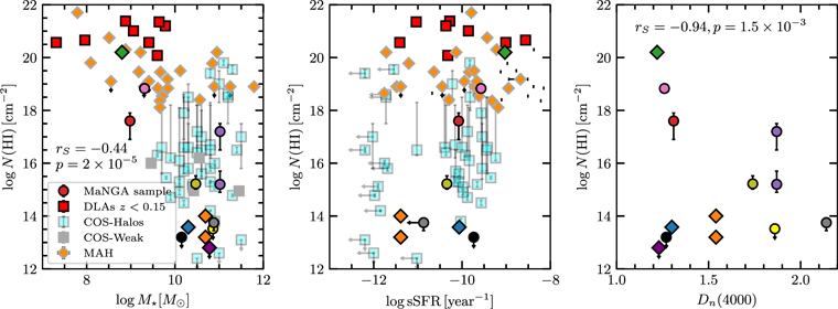
Figure 9. The comparison of H i column density against the stellar mass (left panel), the specific star formation rate (sSFR, middle panel), and the Dn (4000) index (right panel). The symbols are the same as those in Figure 8. In addition, the large diamonds represent our AGN sight lines with "zero impact parameter." The H i column density is anticorrelated with the galaxy stellar mass, but not with sSFR. The quasar sight lines suggest N(H I) decreasing sharply with increasing Dn (4000) (excluding the nondetection of 1-549490 due to the large impact parameter). This indicates the connection of the gas content at very large radii to the star formation history in the center of the galaxy.
Download figure:
Standard image High-resolution imageAbsorption systems with a high H i column density are more likely related to low-stellar-mass galaxies (Kulkarni et al. 2022), while systems with a lower H i column density are associated with the halos of more massive galaxies (e.g., Kulkarni et al. 2010; Tumlinson et al. 2013; Augustin et al. 2018).
The MaNGA galaxies from our sample also follow this trend. Three systems with the highest H i column density (N(H I) ≥ 1018 cm−2) are observed near galaxies with M* ≤ 109 M⊙, while the other systems correspond to high stellar mass galaxies with M* ≃ 1010–1011 M⊙. For the sample of low-redshift z < 0.35 systems (our data; Tumlinson et al. 2013; Kulkarni et al. 2022), we obtain a correlation coefficient rS = − 0.34 and p-value of 5 × 10⁻³, for the entire sample, including MUSE-ALMA observations, rS = − 0.44 and p = 2 × 10⁻⁵. We do not see a difference in the H i content for galaxies with low or high sSFRs. However, a strong negative correlation is observed between the sSFR and stellar mass for AGNs in all of the samples examined here, including our own galaxies and those from the literature (rS = − 0.66, p = 2 × 10⁻⁹).
We also report a strong dependence of N(H I) decreasing with increasing Dn (4000) for quasar sight lines—discounting the nondetection of 1-564490 due to a large impact parameter. The Spearman rank-order correlation coefficient is rS = − 0.94, and the p-value is 0.015. It is interesting that this correlation connects the gas content at very large radii to the star formation history in the center of the galaxy. We suspect we would see the same thing with sSFR if we had measures of sSFR for the three quasar sight-line galaxies with Dn (4000) > 1.7. For galaxy sight lines (when we get the spectrum from the central AGN), we do no see a such dependence probably due to the contamination of the observed spectra by the AGN.
Comparing the correlations between N(H I) and b, M*, Dn (4000) we believe that a primary correlation is likely with stellar mass. Higher-mass galaxies have a higher Dn (4000) index, and their higher past star formation activity is expected to affect cool gas around them, both because cool gas is consumed in star formation and because AGN radiation and stellar winds blow out gas around these galaxies. We do not have many observations of cool gas around massive galaxies at low impact parameters to check this statement in further detail.
4.3. Galaxy Geometry and Kinematics
At the spectral resolution of COS G130M, we can obtain fairly reliable velocity profiles for the absorbing gas along the sight line through the galaxy. This can be compared with kinematics of the ionized gas from MaNGA data. With this in mind, we used the radial velocity maps of the stellar disk and Hα gas for our galaxies to reconstruct the position of the quasar sight lines relative to the gaseous disks of the galaxies and examined the correspondence between the radial velocities of the absorbers and the rotation of the galactic gaseous disks.
First, we fitted both the gas velocity map (Hα
line emission) and the stellar velocity map with symmetric models of thin disk rotation. This formalism was described in Section 2.3.2. We choose the best fit, giving priority to the joint fit (stellar+Hα
emission) first, followed by the Hα
emission-line fit, using only the stellar fit if others did not fit. The position angle (PA), inclination angle (i), and maximal rotation velocities ( ) are presented in Table 4. The fitted velocity map and rotation curve for each galaxy are shown in Figures 18–26.
Table 4. Properties of MaNGA Galaxies
| MaNGA | zgal | Re | [O/H] | ∇R[O/H] |

| ∇R[q] |
 a
a
| PA | Incl. | ϕstand b | ϕmodel c |
|---|---|---|---|---|---|---|---|---|---|---|---|
| ID | (kpc) | (10−3 kpc−1) | (10−3 kpc−1) | (km s−1) | (deg) | (deg) | (deg) | (deg) | |||
| 1-71974 | 0.03316 | 4.9 | 0.31 ± 0.04 | −7 ± 2 | 7.16 ± 0.07 | −13 ± 2 | 151 | 147 | 33 |

|

|
| 1-385099 | 0.02866 | 5.4 | N/A | N/A | N/A | N/A | 200 | 21 | 32 |

|

|
| 1-585207 | 0.02825 | 2.4 | N/A | N/A | N/A | N/A | 155 | 13 | 47 |

|

|
| 12-192116 | 0.02615 | 3.3 | −0.25 ± 0.08 | −18 ± 2 | 7.05 ± 0.20 | −40 ± 2 | 64 | 141 | 36 |

|

|
| 1-594755 | 0.03493 | 1.3 | N/A | N/A | N/A | N/A | 144 | 162 | 22 |

|

|
| 1-575668 | 0.06018 | 10.6 | N/A | N/A | N/A | N/A | 500 | 172 | 8 |

|

|
| 1-166736 | 0.01708 | 3.4 | −0.16 ± 0.10 | −18 ± 8 | 6.96 ± 0.18 | −8 ± 1 | 58 | 156 | 53 |

|

|
| 1-180522 | 0.02014 | 4.1 | 0.06 ± 0.07 | −26 ± 2 | 7.02 ± 0.12 | 3 ± 1 | 124 | 122 | 74 |

|

|
| 1-635629 | 0.01989 | 1.7 | 0.35 ± 0.05 | −14 ± 4 | 7.04 ± 0.10 | −50 ± 5 | 124 | 16 | 65 |

|

|
| 1-561034 | 0.09008 | 6.0 | N/A | N/A | N/A | N/A | 236 | 61 | 50 |

|

|
| 1-113242 | 0.04372 | 5.5 | N/A | N/A | N/A | N/A | 550 | 12 | 26 |

|

|
| 1-44487 | 0.03157 | 6.2 | 0.33 ± 0.05 | −14 ± 1 | 7.06 ± 0.10 | −11 ± 1 | 225 | 25 | 78 |

|

|
| 1-564490 | 0.02588 | 5.7 | 0.36 ± 0.05 | −20 ± 2 | 7.10 ± 0.13 | −60 ± 3 | 150 | 129 | 52 |

|

|
Notes.
a The maximal rotation velocity of the galaxy derived from fitting the "arctan" model. b The elevation angle derived by the standard method. c The elevation angle using the model of gas distribution around the galaxy.Download table as: ASCIITypeset image
4.3.1. Elevation Angle and the Position of Absorbers
The analysis of velocity maps gives us the orientation of the galactic disk relative to the quasar/or galaxy sight line. Here we determine the orientation of absorption system along the quasar sight line with respect to disk plane. To be consistent with Péroux et al. (2020), we adopt (ϕ) to be the elevation angle (90° − polar angle) or latitude with respect to the disk plane and (θ) to be the deprojected angle in the disk plane with respect to the major axis. 19
We estimated the elevation angle (ϕ) of absorption systems in two ways:
(a) using the standard approach as the angle between the galaxy's major axis and the line joining the galactic center to the quasar on the sky plane (Bouché et al. 2012), and
(b) by integrating the elevation angle along the quasar sight line using a model for the gas distribution around the galaxy. In this approach, we assume that the probability of detecting gas absorption along the sight line can be described as follows:

where (r, ϕ) are the radial coordinates and elevation angle of the point along the sight line, C is a normalization coefficient, fΩ = 1/r2 characterizes the decrease in the gas cross section with increasing distance from the galactic center (lower solid angles are probed at larger distances), and fr and fϕ are model distributions of the gas density around the galaxy. For f(r), we adopt the Navarro–Frenk–White halo density profile (Navarro et al. 1997)

with the parameter rs = 6Re . For the elevation angle distribution fϕ , we adopt

where  is a Gaussian distribution with a mean μ and a width σ. Thus, fϕ
is a bimodal distribution with two peaks, one near the galaxy plane and the other near the polar axis, with opening angles of about 30°, consistent with the range of outflow opening angles from
is a Gaussian distribution with a mean μ and a width σ. Thus, fϕ
is a bimodal distribution with two peaks, one near the galaxy plane and the other near the polar axis, with opening angles of about 30°, consistent with the range of outflow opening angles from  to 45° estimated from galaxy spectra with outflow detections (e.g., Martin et al. 2012). Using the probability function of Equation (7), we calculate the mean value of the elevation angle as:

where x is the coordinate along the quasar sight line.
Figure 10 compares these two estimates of the elevation angle. The values agree mostly within the uncertainties. Approach (b) usually predicts lower elevation angles, because it takes into account a higher probability of detection for directions along the galactic plane, while the standard method corresponds to the direction with the smallest impact parameter. For galaxy sight lines (i.e., those with zero impact parameters), we estimated the elevation angle of absorption systems as (π/2) − i, where i is the inclination angle of the galaxy. Using approach (b), we also calculated the deprojected radial coordinate of the absorption system in the disk plane (d) and height of the absorption system above the disk plane (h) as follows:

where r is the radial coordinate of the point along the sight line with the highest probability f(r, ϕ).

Figure 10. A comparison of elevation angles derived by the two methods: from the modeling of gas distribution around the galaxy (vertical axis) and by the standard method (horizontal axis). See details in text. The colors and shapes of the symbols are the same as in previous figures.
Download figure:
Standard image High-resolution image4.4. Gas Kinematics
4.4.1. Quasar Sight Lines
We now compare the absorber velocities in the five quasar sight lines that show absorption detections with the corresponding best-fit models of galactic disk rotation in six MaNGA galaxies. Using the fits to MaNGA emission-line velocities maps, we calculate the radial velocity of the galactic disk along the direction toward the quasar sight line. The comparison is shown in Figure 11. We show both the components seen in H i alone and the components seen in H i as well as metals. Additionally, we show each of these quasar–galaxy pairs in Figures 18, 19, 21, 22, and 23 in Appendix B.

Figure 11. The left panel shows the difference between radial velocities of H i absorption components in quasar sight lines and predicted velocity of galaxy rotational models are shown as a function of radial coordinate. Circles and squares represent components with both H i and metal lines and only H i, respectively. The color encodes the H i column density of the components. The horizontal dotted lines show the range of velocities from −50 to 50 km s−1. The middle panel is the same as the left panel, but shows the velocity offset in units of the predicted velocity of galaxy rotational models. Dotted lines represent the ±1 offsets relative to the predicted velocity (offset = 0). The right panel shows the radial velocity of absorption calculated in the galaxy rest frame as a function of the radial coordinate. The symbols are the same as in other panels. Color encodes the stellar mass of nearby galaxies. The curves show the escape velocity as a function of the distance for stellar masses of  . See the text for more details.
Download figure:
Standard image High-resolution imageFor three of the six galaxies (1-166736, 1-180522, and 1-575668) there is good agreement between the velocities of the strongest H i absorption components and the predicted radial velocities of the galactic disks within ±50 km s−1. We note that these quasar sight lines are located within 10 effective radii from the corresponding galaxies. For two other galaxies (1-635629 and 1-113242), the absorption velocity is in the opposite direction to that expected from the galactic disk rotation. And for one galaxy (1-44487), the absorption components are spread over a wide range ∼350 km s−1. However, this range is comparable with the velocity of galaxy rotation in the quasar sight line direction (∼250 km s−1).
The middle panel of Figure 11 shows the velocity offset normalized by the predicted galactic disk rotation radial velocity at the appropriate distance. It is clear that this normalized velocity offset is within ∼±1 in most cases. In other words, the absorbing gas velocity is generally consistent with corotation with the galactic disk within ∼25 effective radii.
We comment now on the difference between the kinematics of the absorbing gas components seen in both H i and metal lines, and those seen in only H i lines. In all cases, only H i absorption is observed in components with a low H i column density (∼1013 cm−2), whereas absorption in both H i and metals is observed in components with N(H I) > 1015 cm−2. Thus the absence of metal absorption in only H i components is likely to be due to a limit in the sensitivity for detecting weak lines at the S/N reached. Second, two out of the three cases of large normalized velocity offsets are for H i-only absorbers, possibly suggesting that the H i-only absorption may be related to the galaxy halo or the IGM and thus not participate in the galaxy disk's rotation. The metal-bearing H i absorbers are, however, likely to relate to the disk gas and hence corotate with it.
It is of interest to understand whether or not the H i-only absorption is bound to the galaxies. To examine this, we compare the velocity offsets of the absorbers relative to the systemic redshifts of the galaxies with the expected escape velocities at the impact parameters of the quasar sight lines. To estimate the escape velocity at a distance r from the center of galaxy with stellar mass M* we used the methodology described in Kulkarni et al. (2022). The right panel of Figure 11 shows the velocity offsets with respect to galactic redshifts
20
for the quasar sight lines in our sample. The curves show the escape velocity as a function of the distance for stellar masses of  , 9.5, 10, 10.5, and 11. There are two galaxies (1-166736 and 1-44487), for which the velocity offset of only H i components exceeds the escape velocity at the corresponding distance: these components may be associated with unbound outflow or be formed from the IGM. At the same time, the other two cases of only H i absorption correspond to more massive galaxies (1-575668 and 1-113242, M* ∼ 1011
M⊙), where the gas is likely bound to the galaxies. The metal-bearing H i absorbers appear to be bound to the galaxies (only one such absorber, associated with the galaxy 1-180522, has a radial velocity very close to the escape velocity).
, 9.5, 10, 10.5, and 11. There are two galaxies (1-166736 and 1-44487), for which the velocity offset of only H i components exceeds the escape velocity at the corresponding distance: these components may be associated with unbound outflow or be formed from the IGM. At the same time, the other two cases of only H i absorption correspond to more massive galaxies (1-575668 and 1-113242, M* ∼ 1011
M⊙), where the gas is likely bound to the galaxies. The metal-bearing H i absorbers appear to be bound to the galaxies (only one such absorber, associated with the galaxy 1-180522, has a radial velocity very close to the escape velocity).
The most interesting case is that of the quasar−galaxy pair, J2130−0025 and 1−180522. The galaxy is observed with a high inclination angle of about 70° (nearly "edge-on"), and the quasar sight line is located very close to the galactic plane (elevation angle is ∼3° ± 7°) at ∼8.5 effective radii. In this case, we find very good consistency between the absorption velocity and the galactic disk rotation velocity. The sight line of J2130−0025 is also close to another galaxy, 1-635629, which has a similar redshift as 1-180522, but is located at a distance of about 39 effective radii. In fact, the velocity of the absorption system is opposite to the expected disk velocity for 1-635629. We therefore infer that the absorption system corresponds to only one galaxy, 1-180522, and that there is no detection for 1-635629.
In two cases, 1-166736 and 1-575668, we also detected high-velocity components with velocity offset v ≃ − 200 km s−1 and +400 km s−1, respectively. Since these components have low H i column densities ∼1013.5 cm−2, they are likely to be highly ionized clouds. In the case of 1-166736, the direction of the cloud velocity is consistent with the direction of the gas outflow, which can be detected with the targeted quasar sight line (see Figure 18). Assuming that the galaxy has two cone-shaped outflows from the center in both directions along the polar axis, the quasar sight line can probe the outflow only in the direction to the observer (with negative radial velocity) and cannot probe the outflow in the opposite direction (with positive radial velocity), because this part of the sight line is located far from the galactic center; see the "Z–Y" projection in Figure 18. In the second case, galaxy 1-575668 is observed nearly "face-on" with a small inclination ∼8° (see Figure 22). The quasar sight line can probe both outflows; however, the distance between the sight line and galactic polar axis is lower from the side of positive velocity outflow. Therefore, the probability of detecting an absorption system with a positive radial velocity is higher, which is in line with observations.
Two other galaxies, 1-44487, and 1-113242 show velocity offsets, with the velocity of the strongest H i components about −100 and +200 km s−1, respectively. In both of these cases, the quasar sight lines are located at ∼23 effective radii, which is about twice the distance of the first group, where we detect a good agreement. In the case of 1-44487, we find at least four absorption components with velocities spanning a wide range of ∼300 km s−1. Since the galaxy is relatively far from the quasar and the absorption has a complex structure, relatively high N(H I) ∼ 1015 cm−2 and supersolar metallicity ([X/H] = + 0.8), we checked the area around the quasar for other galaxies with similar redshift, but found none. However, we note that this galaxy is merging with another smaller galaxy, and it is likely that the observed high metallicity is due to outflows in a region of enhanced star formation caused by the merger.
Summing up, we find consistency with gas corotation along with the galactic disk within at least 10 effective radii in most cases. The sign of the velocity of higher-velocity absorption, when detected, is consistent with the direction of the central galactic outflows, which have a higher probability of detection in these sight lines. For quasar sight lines at larger impact parameters, the situation is less clear.
4.4.2. AGN Sight Lines
We now discuss the gas kinematics for three of the four AGN sight lines (those with zero impact parameters) in our sample that show detections of absorption. We observed the AGNs of these galaxies at elevation angles of about 60°. These directions are within the outflow opening angles ( to 45°) reported by Martin et al. (2012), and therefore these sight lines can probe gas in the central outflows. Of course, the AGN sight lines can also probe gas in the CGM/IGM at a large distance, and these scenarios can be difficult to distinguish.
For two sight lines (1-71974 and 1-385099), the H i absorption lines are weak (N(H I) ∼ 1013–1014 cm−2) and blueshifted by −50 and −250 km s−1, and by −50 and −750 km s−1, respectively, with respect to the galactic redshift. The velocity of the low-velocity components is comparable to the galactic disk rotation velocity measured by MaNGA (∼100 km s−1). The high-velocity components in these sight lines cannot be described by the galactic disk rotation model. The absorption in these components is characterized by high ionization and high metallicity, about two orders higher than measured for the absorption in the quasar sight lines. The high ionization could potentially arise in either outflowing gas ionized by the AGN radiation, or in low-density IGM gas. However, the high metallicity suggests that the outflow scenario is more likely, since the IGM is not expected to be metal-rich.
The third AGN sight line, 12-192116, probes gas with high neutral hydrogen content (N(H I) ∼ 1020.2 cm−2), low ionization, and low metallicity ([X/H] ≃ − 1). This absorption cannot be related to the galactic disk due to the high elevation angle, but may arise in a "satellite" galaxy, similar to what may be observed by extragalactic observers as absorption from the Magellanic Clouds toward the center of the MW. Alternatively, this absorption could arise in gas clouds tidally interacting with the galaxy, similar to high-velocity clouds (HVCs) with N(H I) > 1020 cm−2 (e.g., Putman et al. 2002; Hsu et al. 2011).
We also note that in the spectrum of the AGN of 1-385099, we find additional absorption of H i at a very high velocity v ≃ − 800 km s−1. Since this galaxy is part of a group along with at least two other galaxies, 1-585207 and SDSS J083804.94+245327, with similar redshifts and projected distances of ∼50 kpc from the observed sight line, the HVC we detect may correspond to the intra-group gas perturbed due to the interaction of these galaxies. The SDSS image of this region shows the presence of long tidal tails for all galaxies (see, e.g., Figure 1). As an analog from the local universe, we note that absorption at such high velocities (much higher than the velocities associated with the MW's halo gas or the Magellanic Stream) is observed in the Sculptor group galaxies (e.g., Putman et al. 2003).
4.5. Metallicity Gradient
Combining the cool-gas metallicity along with the warm-gas metallicity is essential to building a complete census of metals in and around galaxies. While such comparisons of cool-gas metallicity and warm-gas metallicity have been performed in IFS studies of quasar absorbers at higher redshifts (e.g., Péroux et al. 2012, 2014), such comparisons have not been performed for the z ∼ 0 galaxies that have much more detailed information. Our study of the CGM of MaNGA galaxies offers an opportunity to study differences in metallicity in the inner versus outer parts of galaxies in some of the closest venues available, and can thus provide fresh insights into processes affecting galactic evolution.
With this in mind, we study how the gradient of IZI metallicity derived from the fit to MaNGA emission-line maps within a few effective radii corresponds to the metallicity measured in the absorption systems along the targeted sight lines. Simulations predict a change in the metallicity gradient from an almost linear relation in the galactic disk (e.g., Mingozzi et al. 2020) to a flatter behavior in the CGM (Péroux et al. 2020). Our sight lines probe the transition region between these two limits. Figure 12 shows the comparison for five galaxies, where we simultaneously measured metallicity in the galaxy and the absorption system. For the absorption systems, we show the average metallicity and local metallicity in individual components derived from fits with the cloudy photoionization models (see Section 3.1). For the studied systems, the average and local values are in good agreement with each other. For absorption in quasar sight lines, we use the deprojected radial coordinate of the absorption system in the disk plane (d) calculated in Section 4.3.1. For the galaxies, we calculate the gradient of the IZI metallicity in the galactic disk in two ways: (i) by averaging over all directions and (ii) by averaging over only the spaxels within ±15° opening angle around the direction to the quasar sight line. The second way is possible only for quasar−galaxy pairs, when we have a preferred direction. The gradients are shown by gray and pink lines, respectively. In Figures 18–26 we also present the IZI metallicity maps and fits to their radial profiles. The deprojected radial coordinate of each spaxel in the MaNGA maps was derived from the best-fit model of the galactic radial velocity map (see Section 2.3.2). The model for the metallicity radial gradient in the CGM has been taken from post-processing of the TNG50 galaxy simulation presented by Péroux et al. (2020) in their Figure 5. It represents measurements of the CGM metallicity in the TNG50 simulation at four values of impact parameter: b = 25, 50, 100, and 200 kpc, and four values of azimuthal angle: 0°, 30°, 60°, and 90°. Other parameters were set to the appropriate values, which are: redshift z = 0, stellar mass M* equal to stellar mass of the MaNGA galaxies. The metallicity is decreased by 0.4–0.7 dex between 25 and 200 kpc in outflow (at 90°) and galactic disk (at 0°) directions, respectively. It is greater than the metallicity gradient due to the elevation angle change, 0.1–0.4 dex at 25 and 200 kpc, respectively. Péroux et al. (2020) suggested that this is because fountains do not yet promote metal mixing over the full volume (i.e., range of elevation angles) at the distances b ∼ 100 kpc, as occurs closer to the galaxy. For the absorption systems in the AGN sight lines, we show the level of metallicity in the absorption system with the horizontal red line, since the distance of the absorbing region from the galactic center is not known.

Figure 12. Comparison of the gradient of IZI metallicity derived from fitting to MaNGA emission-line maps and metallicity measured in absorption systems. The left panels show the comparison for absorption systems in quasar sight lines with nonzero impact parameter. The right panels show the comparison for absorption systems along galaxy/AGN sight lines with zero impact parameter. Red and pink circles represent the average metallicity in absorption systems, and the metallicity in individual components, respectively. The black solid line and black shaded area in each panel show the linear gradient of IZI metallicity averaged over the elevation angle. The pink solid line and pink shaded area in left panels show the linear gradient of IZI metallicity in the direction to the quasar sight line. The orange, blue, green, and red dashed curves show the model distribution of metallicity in the CGM from the TNG50 simulation (see Figure 5 in Péroux et al. 2020), derived at different azimuthal angles 0°, 30°, 60°, and 90°, respectively, and four values of impact parameter (25, 50, 100, and 200 kpc). The model is adopted to z = 0 and the galaxy stellar mass. For two galaxies (1-180522 and 1-166736), the quasar sight lines more likely probe gas near the galactic plane. Galaxy 1-44487 is an interacting galaxy, and this activity may result in a high metallicity measured in the absorption system at high impact parameter. AGN sight lines likely probe a high-metallicity central outflow (1-71974) and gas in a "satellite" galaxy (12-192116); see the text.
Download figure:
Standard image High-resolution imageComparing the five panels of Figure 12, we note that we confirm the increase of the galactic central metallicity with the stellar mass, previously reported by Mingozzi et al. (2020) for star-forming galaxies from the MaNGA survey. Second, we detect a consistency of metallicity in the absorption system in the quasar sight lines with the prediction from the metallicity gradient for two galaxies (1-180522 and 1-166736). These quasar sight lines (J2130−0025 and J0950+4309, respectively) more likely probe gas near the galactic plane at ∼7 and ∼8 effective radii. In these cases, the metallicity gradient measured from the fit to MaNGA maps (at 2–3 effective radii) can persist over a longer distance. The metallicities in these absorption systems are also consistent with the prediction for the CGM metallicity showing that the simulations may reproduce the CGM properties well. For the third galaxy, 1-44487, we measure about 2 orders of magnitude higher metallicity, than the predictions from the "galaxy" gradient. Since the impact parameter is high (137 kpc), this quasar sight line should probe metallicity in the CGM, which is expected to be higher than that predicted from the "galaxy" gradient. For stellar mass ∼1010.5 M⊙, the CGM metallicity is expected to be about [X/H] = − 0.5, which is still ∼1.5 orders of magnitude lower than the measured value. This discrepancy may result from the activity of the merged galaxy. For the absorption systems located toward the galactic centers of 1-71974 and 12-192116 galaxies, we found an excess of metallicity in the first case, which can be caused by a high-metallicity central outflow, and one order lower metallicity in the second, which may be the metallicity of the "satellite" galaxy or an HVC (see the discussion of this case in Section 4.4.2.).
4.6. Dependence of Metallicity on the Elevation Angle
Hydrodynamic simulations of galactic evolution predict an increase of CGM metallicity with the elevation angle with respect to the disk plane (see, e.g., Péroux et al. 2020). Metal-free gas is expected to fall into the galaxy along directions close to the galactic disk plane, while metal-rich gas is expected to flows out of the galactic disk in directions near the perpendicular to the plane by stellar winds and supernova explosions. Therefore, we can expect an increase of gas metallicity with the elevation angle (e.g., see Figure 5 in Péroux et al. 2020). The angular gradient of metallicity is predicted to be around +0.4 dex/90° for galaxies at z ≃ 0.
Figure 13 presents the dependence of metallicity in absorption systems on the elevation angle in our sample. For each system, we show the metallicity measured in the velocity components to test the variation of physical conditions. We also show the two estimates of the elevation angle discussed in Section 4.3.1 ((a) from the standard method, and (b) from the model of gas distribution). We find that, if we consider the metallicity only in quasar absorption systems (apart from the case of the merged galaxy, 1-44487), we have a good agreement between the observed absorption metallicities and the simulations. The main difference in the measured metallicities is due to the difference in galaxy stellar masses, whereas the gradient with the elevation angle is small. The metallicity measurements in the AGN sight lines should not follow the trend in the simulations, because they probably do not probe the CGM. The galaxy sight lines can probe gas at very low distances and in AGN central ejections, which could describe high metallicity and high ionization of these systems. However these processes were not considered in the simulations by Péroux et al. (2020), van de Voort et al. (2021), and Wendt et al. (2021), meaning no AGN at low M⋆ in simulations. At the same time, the galaxy 12-192116 shows good consistency. In this case, we may be dealing with a galactic absorption system with an unusually large elevation angle, and we suggest that it may be caused by absorption from a "satellite" galaxy, or from metal-poor inflowing gas.
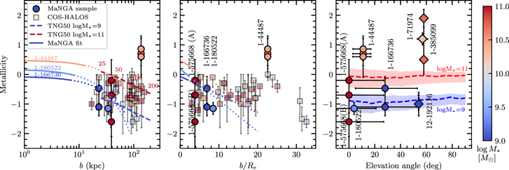
Figure 13. The comparison of metallicity of absorption systems against the impact parameter (left panel), with impact parameter in units of effective radii (middle panel) and elevation angle (right panel). Circles and diamonds represent the metallicity in individual velocity components for the quasar and AGN absorbers, respectively, from our sample. Transparent squares show data from the COS-Halos survey (Tumlinson et al. 2013). The color of symbols denotes the galactic stellar mass. The solid and dotted curves in the left and middle panels show the metallicity gradient in MaNGA observations and its extrapolation to 20 effective radii (as in Figure 12). The dashed lines in the left and right panels show the gradient of metallicity with distance (left) and with elevation angle (right) from galaxy formation simulations (Péroux et al. 2020). The radial gradient was derived at z = 0, for an elevation angle of 0°, and for galaxy stellar masses of 109 M⊙ and 1011 M⊙. The gradient with the elevation angle was derived at z = 0, for b = 25–100 kpc, and for galaxy stellar masses of 109 M⊙ and 1011 M⊙.
Download figure:
Standard image High-resolution imageWe also compare our results with metallicity measurements in the COS-Halos survey (Werk et al. 2014). The effective radii of the COS-Halos galaxies were derived from the relation between the effective radius and the stellar mass by Mowla et al. (2019). We do not detect a significant correlation between [X/H] and b/Re for the joint sample, with a Spearman rank-order correlation coefficient of 0.1 and a p-value of 0.46.
4.7. Ionization Parameter
Figure 14 shows the ionization parameter versus impact parameter and elevation angle for our sample galaxies. We find the ionization parameter to be roughly constant for MaNGA galaxies with a mean of ∼10−3.3 and the dispersion of ∼0.1 dex (see Table 3). On the contrary, the ionization parameter in the absorption systems spans over 2 orders of magnitude above the average galactic ionization. The difference may be primarily due to the difference of gas number density between the ISM (∼102 cm−3; e.g., Mingozzi et al. 2020) and the CGM (∼10−1–10−3 cm−3). The ionization parameter q = nγ
/nH is proportional to the ratio of IUV/nH. Assuming the ionization of the CGM is due to the extragalactic background only (whose intensity is about 10−2 of the average UV galactic radiation), the difference in q parameter is obtained from  , which gives a factor 10–103 for the range of the CGM number densities. The factor will be lower if the galactic UV intensity is stronger than the average UV galactic radiation.
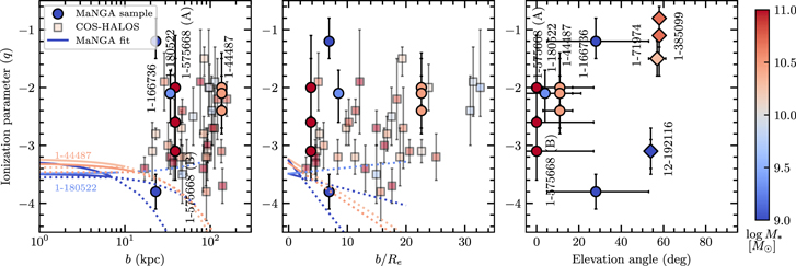
Figure 14. Comparison of gas ionization parameter of absorption systems against the impact parameter (left panel), impact parameter to effective radius (middle panel), and the elevation angle (right panel). The symbols are the same as in Figure 13: circles and diamonds—our sample, transparent squares—from COS-Halos survey. The color of the symbols denotes the galactic stellar mass. The solid and dotted curves in the left and middle panels show the ionization parameter gradient in MaNGA observations and its approximation to 20 effective radii (as in Figure 12).
Download figure:
Standard image High-resolution imageWe did not find much correlation of the ionization parameter of the absorption systems with galactic properties such as stellar mass, SFR, or sSFR. However, it correlates with the elevation angle (see the right panel of Figure 14).
As shown above, quasar sight lines probe gas around galaxies at lower elevation angles and at higher impact parameters than AGN sight lines (1-385099 and 1-71974), and for the former, we found lower ionization parameters. This is consistent with the picture that gas at small elevation angles corresponds to galactic disks (or inflowing gas) and has lower metallicity and lower ionization parameters than the gas observed in absorption at larger elevation angles (which may arise in outflows with higher ionization fractions and higher metallicity). For the quasar sight line J0950+4309, which probes the gas around the galaxy 1-166736 at a moderate elevation angle, we found a large difference in the ionization parameter between the components seen in the Si ii and Si iii absorption lines. The low-ionization gas traced by Si ii may correspond to the galactic disk, while the highly ionized gas observed only in Si iii may correspond to the CGM. The higher ionization component in 1-166736 is consistent with the trend observed between the ionization parameter and the elevation angle.
We also compare our data with measurements of the ionization parameter in the COS-Halos survey (Werk et al. 2014). Our results are consistent with their results and cover the same range of ionization parameter. However, we do not confirm the trend log q = −2.2 ± 0.3 + (0.8 ± 0.3) × log (R/Rvir) reported by Werk et al. (2014; based on the points at very low and high impact parameters). Combining our sample with the COS-Halos sample, we find that the correlation of ionization parameter with impact parameter is not statistically significant with a Spearman rank-order correlation coefficient of 0.2 and p-value 0.16. Indeed, high-ionization parameters, on average, correspond to a higher impact parameter. However, there is a large scatter of q parameters that likely reflects the inhomogeneity of physical conditions in the CGM of different galaxies.
5. Conclusions
We have measured the CGM properties out to 25 effective radii using HST/COS spectroscopy of quasars and AGNs about a sample of low-redshift galaxies with exquisite data from the MaNGA survey. We detected the associated absorption for 11 of 14 galaxies in our sample. In three cases, the absorption was detected in the sight lines toward the bright source near the galactic center; in other cases, the absorption was detected in background quasar sight lines at an impact parameter of 23–137 kpc. For the AGN sight lines, we detected a strong H i absorption (N(H I) ≃ 1020.2 cm−2) in only one case. In two other cases, we found weak H i absorption (N(H I) ≃ 1013 cm−2), which may be related to high-metallicity and high-ionization gas in the central outflow. Our quasar sight lines show H i absorption with a wide range of N(H I) ≃ 1013–1019 cm−2.
To summarize, our main results are as follows:
- 1.
- 2.Our data also agree well with other spectroscopic studies of halos of galaxies at low redshift z < 0.3 (COS-Halos by Tumlinson et al. 2013; COS-Weak by Muzahid et al. 2018) and of the gas in "galaxies on top of quasars" (in the close vicinity of low-z galaxies within impact parameters ∼1–7 kpc; Kulkarni et al. 2022).
- 3.We confirm the anticorrelation between the H i column density and the galaxy stellar mass that was previously reported by Kulkarni et al. (2022).
- 4.We report a strong dependence of N(H I) decreasing with increasing Dn (4000) index of the host galaxies for quasar sight lines, which may be a result of past star formation activity having consumed or blown out cool gas from the CGM.
- 5.A comparison of absorption velocities with radial velocity maps of ionized gas line emission in galaxies shows consistency with corotation of the strong H i absorption component with the disk out to ∼10 effective radii (within ±50 km s−1) and ∼25 effective radii (within ±1 galactic disk rotational velocity). The components with only H i absorption (without associated metal lines) are likely to have a high-velocity shift and in some cases may be unbound to the galaxy.
- 6.Comparing the observed CGM properties with the galaxy properties from MaNGA maps, we estimate the gradients in metallicity and ionization parameters. The measurements of absorption metallicities in individual quasar sight lines correspond well with the gradient of metallicity in the galactic disk derived from MaNGA observations. Overall, from our sample and previous studies, we find a lower metallicity in the quasar sight lines with respect to the AGN sight lines. The difference is consistent with the predictions of the CGM metallicity from TNG50 simulations (Péroux et al. 2020).The ionization parameter in absorption systems is on average 1 order of magnitude higher than the galactic value (q ∼ 10−3.5). The measurements in our sample and previous studies do not show a statistically significant gradient of the ionization parameter with distance from the galaxy. This indicates a strong inhomogeneity of the physical conditions in the CGM (number density and intensity of H i-ionized radiation). However, the data are consistent with an increasing ionization parameter with increasing elevation angle.
Our data offer the first detailed comparisons of CGM properties with extrapolations of detailed galaxy maps. While our data offer a number of interesting insights into the exchange of gas and metals between galaxies and their CGM, our current sample is still small. Observations of the CGM of many more galaxies mapped with IFS are essential to more fully understand how galaxies interact with their CGM.
Acknowledgments
This work is supported by a grant from the Space Telescope Science Institute for GO program 16242 (PI V. Kulkarni). Additional partial support is also gratefully acknowledged from the US National Science Foundation grant AST/2007538 and NASA grant 80NSSC20K0887 (PI V. Kulkarni).
We would like to thank Francesco Belfiore and Kyle Westfall for helpful advice on analyzing the MaNGA emission-line ratios. We thank Sergei Balashev for sharing a version of the Spectro Voigt profile fitting code, before its official release. We are grateful to an anonymous referee for providing a careful reading and constructive suggestions that have helped to improve this paper.
Funding for the Sloan Digital Sky Survey IV has been provided by the Alfred P. Sloan Foundation, the U.S. Department of Energy Office of Science, and the Participating Institutions. SDSS-IV acknowledges support and resources from the Center for High Performance Computing at the University of Utah. The SDSS website is www.sdss4.org.
SDSS-IV is managed by the Astrophysical Research Consortium for the Participating Institutions of the SDSS Collaboration including the Brazilian Participation Group, the Carnegie Institution for Science, Carnegie Mellon University, Center for Astrophysics, Harvard & Smithsonian, the Chilean Participation Group, the French Participation Group, Instituto de Astrofísica de Canarias, The Johns Hopkins University, Kavli Institute for the Physics and Mathematics of the Universe (IPMU)/University of Tokyo, the Korean Participation Group, Lawrence Berkeley National Laboratory, Leibniz Institut für Astrophysik Potsdam (AIP), Max-Planck-Institut für Astronomie (MPIA Heidelberg), Max-Planck-Institut für Astrophysik (MPA Garching), Max-Planck-Institut für Extraterrestrische Physik (MPE), National Astronomical Observatories of China, New Mexico State University, New York University, University of Notre Dame, Observatário Nacional/MCTI, The Ohio State University, Pennsylvania State University, Shanghai Astronomical Observatory, United Kingdom Participation Group, Universidad Nacional Autónoma de México, University of Arizona, University of Colorado Boulder, University of Oxford, University of Portsmouth, University of Utah, University of Virginia, University of Washington, University of Wisconsin, Vanderbilt University, and Yale University, and the Collaboration Overview Start Guide Affiliate Institutions Key People in SDSS Collaboration Council Committee on Inclusiveness Architects SDSS-IV Survey Science Teams and Working Groups Code of Conduct Publication Policy How to Cite SDSS External Collaborator Policy.
Data Availability
Data directly related to this publication and its figures can be requested from the authors. The MaNGA data used in this paper can be downloaded from the MaNGA public archives. The HST data used in this paper can be found in MAST: doi:10.17909/zpy3-w565.
Appendix A: Flux Uncertainty Estimate
The flux errors of the HST/COS spectra originates in three sources: the errors associate`d with flat-field response, the Poisson error in the counts from the object flux (galaxy/quasar), and the Poisson error in the counts from the background flux (e.g., Johnson et al. 2021). In our case, the first and third contributions are much smaller then the second. However, for faint sources, the object counts are low. Therefore, the problem is to estimate the upper and lower flux errors for the Poisson distribution in the case of a small number of counts. The standard CalCOS pipeline uses an asymmetric uncertainty based on the frequentist-confidence method (see Gehrels 1986) and described by
and
where N is the number of observed counts. We found that for low count numbers (<10), these uncertainties are overestimated by the standard CalCOS pipeline. Therefore, we reevaluated the uncertainties by the maximum probability estimate (MPE) method.
A comparison of the uncertainties estimated using the two methods is shown for the case N = 3 in Figure 15. The lower uncertainties are similar, while the upper uncertainties derived by the MPE method are about two times lower than those derived by the frequentist-confidence method. We note that both estimates correspond to 68% confidence interval (1σ); however, the frequentist-confidence estimate is shifted to higher values. The relative difference between the uncertainty estimates decreases with an increase in the number of counts (N), and is small for N > 20. The top panel of Figure 16 shows the upper and lower uncertainty estimates from the two methods. We adopt the uncertainty estimates in integral number of counts, since this seems more physical. The bottom panel shows a comparison of the ratio of uncertainties to the standard deviation for the Poisson distribution. The standard deviation was calculated independently for fluxes above and below the mean value (N). The estimates correspond well to the standard deviation over the entire range of N.
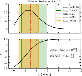
Figure 15. Comparison of the estimates of positive and negative uncertainties for the Poisson distribution in the case of a low number of counts (N = 3). The top and bottom panels show the probability distribution function (PDF) and the cumulative distribution function (CDF), respectively. The vertical red dashed lines show the mean value. The green lines and green dashed area represent the confidence interval derived by the CalCOS pipeline. The yellow lines and yellow dashed area represent the confidence interval derived by the maximum probability estimate (MPE) method.
Download figure:
Standard image High-resolution image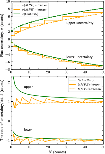
Figure 16. The top panel shows the comparison of positive and negative uncertainties for the Poisson distribution for different values of N. The dashed and solid yellow curves show our estimate, which is represented by a fraction in an integer number of samples. The green line represents the CalCOS estimate. The bottom panel shows a comparison of the upper and lower estimates with the standard deviations for the Poisson distribution, calculated independently for the upper and lower outliers.
Download figure:
Standard image High-resolution image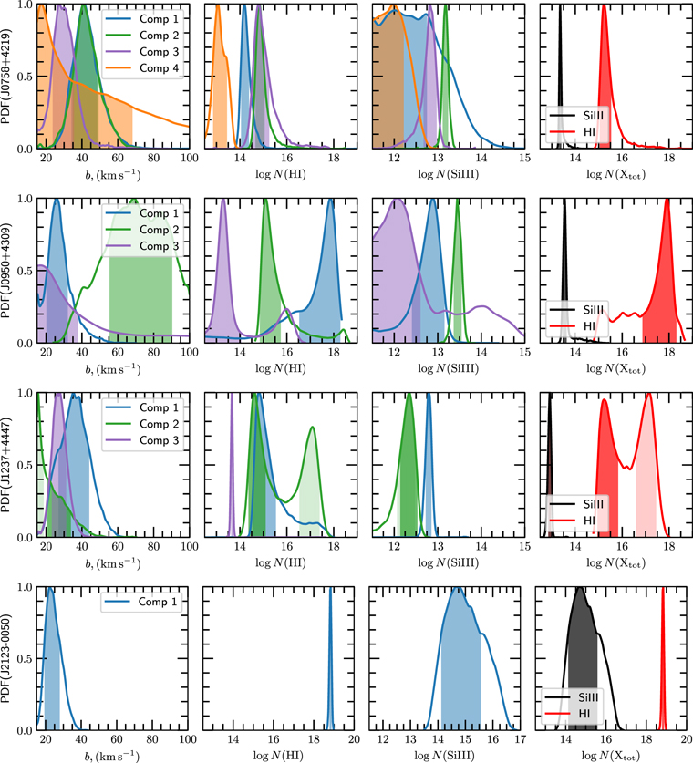
Figure 17. The posterior probability density function (PDF) of fitting parameters of H i and Si iii lines in four HST COS spectra shown in Figure 3. The first three columns from left to right show the PDF of the b-parameter,  , and
, and  . The color of curves corresponds to the color of velocity components in Figure 3. The dashed area represents the 68% confidence interval around the value with the maximum probability. For the case of J1237+4447, the light and heavy dashed areas show two different solutions (see the text). The rightmost column shows the PDF of the total H i column density and the total Si iii column density (summed over the components) by red and black curves, respectively.
Download figure:
Standard image High-resolution imageAppendix B: Absorption-line Analysis Details
In this section we present detailed results of analysis of each absorption system individually. Fit results to absorption systems are shown in Table 5 and Table 6. Figure 17 presents the posterior PDF of fitting parameters for the systems shown in Figure 3. Figures 18–23 show results for quasar–galaxy pairs, Figures 24–35 show results for AGNs. In these figures we compare radial velocity, metallicity, and ionization parameter derived from the fitting to MaNGA maps of the galaxies and those measured from fitting to absorption lines in the absorption system in our HST/COS spectra. We describe the panels in the figures below.
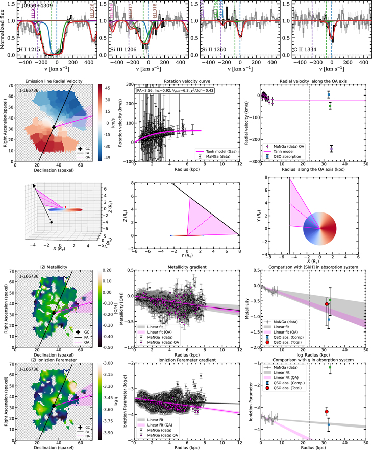
Figure 18. Comparison of radial velocity, metallicity, and ionization parameter derived from the fitting to MaNGA maps of the galaxy 1-166736 and those measured in the absorption system toward the quasar J0950+4309. A detailed description of the panels is presented in Appendix B.
Download figure:
Standard image High-resolution image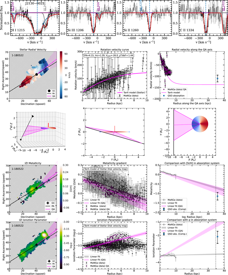
Figure 19. Comparison of radial velocity, metallicity, and ionization parameter derived from the fitting to MaNGA maps of the galaxy 1-180522 and those measured in the absorption system toward the quasar J2130−0025. A detailed description is presented in Appendix B.
Download figure:
Standard image High-resolution image
Figure 20. Comparison of radial velocity, metallicity, and ionization parameter derived from the fitting to MaNGA maps of the galaxy 1-635629 and those measured in the absorption system toward the quasar J2130−0025. A detailed description is presented in Appendix B.
Download figure:
Standard image High-resolution image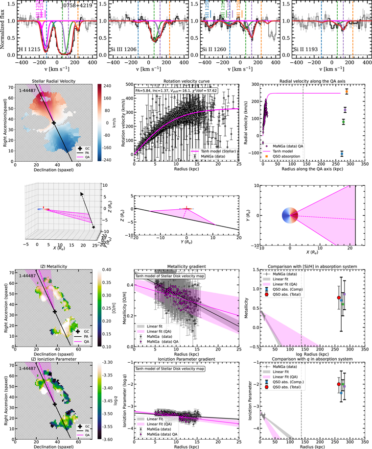
Figure 21. Comparison of radial velocity, metallicity, and ionization parameter derived from the fitting to MaNGA maps of the galaxy 1-44487 and those measured in the absorption system toward the quasar J0758+4219. A detailed description of the panels is presented in Appendix B.
Download figure:
Standard image High-resolution image
Figure 22. Comparison of radial velocity derived from the fitting to MaNGA maps of the galaxy 1-575668 and those measured in the absorption system toward the quasar J1237+4447. A detailed description of the panels is presented in Appendix B.
Download figure:
Standard image High-resolution image
Figure 23. Comparison of radial velocity derived from the fitting to MaNGA maps of the galaxy 1-113242 and those measured in the absorption system toward the quasar J2106+0909. A detailed description of the panels is presented in Appendix B.
Download figure:
Standard image High-resolution image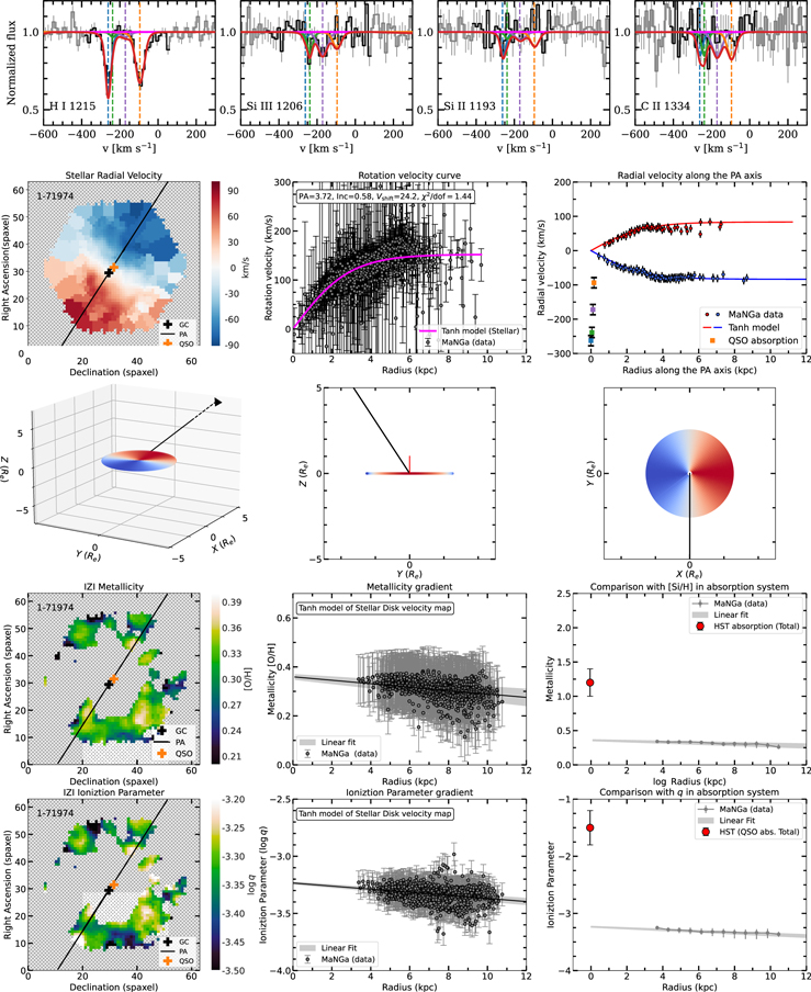
Figure 24. Comparison of radial velocity, metallicity, and ionization parameter derived from the fitting to MaNGA maps of the galaxy 1-71974 and those measured in the absorption system toward the AGN J0755+3911. A detailed description of the panels is presented in Appendix B.
Download figure:
Standard image High-resolution image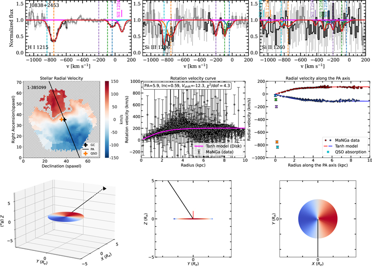
Figure 25. Comparison of radial velocity derived from the fitting to MaNGA maps of the galaxy 1-385099 and those measured in the absorption system toward the quasar J0838+2453. A detailed description of the panels is presented in Appendix B.
Download figure:
Standard image High-resolution image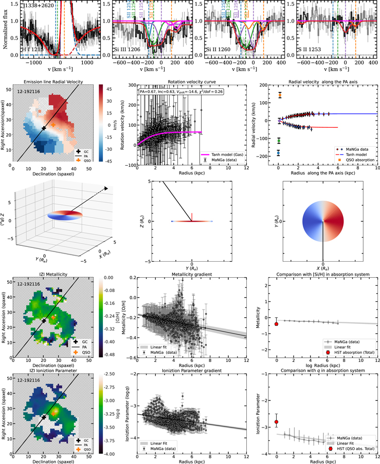
Figure 26. Comparison of radial velocity, metallicity, and ionization parameter derived from the fitting to MaNGA maps of the galaxy 12-192116 and those measured in the absorption system toward the AGN J1338+2620. A detailed description of the panels is presented in Appendix B.
Download figure:
Standard image High-resolution imageThe panels in the top row show the HST COS data for the H i, Si iii, Si ii, and C ii absorption lines and our best fits to these lines. The synthetic profile is shown in red, and the contribution from each component is shown in green, blue, purple, and orange.
The panels in the second row show a comparison of radial velocities. In each case, the left panel shows the MaNGA velocity field (determined from the Hα -line emission or the stellar continuum). The black line represents the positional angle (PA), the pink line and pink shaded area represent the direction to the quasar sight line within opening angle 15°, the black cross represents the position of the center of the disk, and the orange cross represents the position of the AGN (only for AGN sight lines). The second panel shows the galaxy rotation velocity curve, reconstructed using the best fit to the radial velocity map. The circles show measurements from the MaNGA spaxels, and the pink line shows the model. The right panel compares the model of radial velocity in the direction to the quasar (QA) and the velocities of the absorption components. The dashed vertical line represents the value of the impact parameter.
The panels in the third row show the orientation of the quasar sight line with respect to the disk plane. The left panel shows a 3D plot: the quasar sight line is shown by the black line (with the black star denoting the quasar), and the observer is located at the top of the panel. The color of points in the galactic disk corresponds to the value of the radial velocity measured by the observer (the same as in the MaNGA velocity map). The pink shaded area shows the range of the elevation angles corresponding to our probability estimate of the position of the absorption system along the quasar sight line (see Section 4.3.1). The dashed and solid pink lines represent the maximum probability value ( ) and its 1σ uncertainty. The middle and right panels show the Y–Z and X–Y projections of the 3D plot, respectively.
The panels in the fourth row show a comparison of the metallicity of the ionized gas measured from the IZI modeling of MaNGA maps of emission lines and the metallicity of the cool gas from the CLOUDY fitting to metal column densities in the absorption system. The left panel shows the MaNGA maps, in which the lines and symbols are the same as in the first panel in the second row (radial velocity map). The middle panel shows the radial profile of the IZI metallicity (circles with error bars) and the best fit to IZI metallicity gradients by a linear model (black line). The pink line corresponds to the IZI metallicity gradients in the direction of the quasar (QA) within a 15° opening angle. Shaded areas represent 1σ uncertainty. The right panel shows a comparison of the IZI metallicity gradient with metallicity measured in the absorption system (small circles represent values for individual components, and red circle shows the total value).
The panels in the fifth row are similar to the panels in the fourth row, but for the ionization parameter.
Figures 27–31 show the best fits to absorption lines, and Figure 36 shows a comparison of measured total column densities of metals with the values predicted by cloudy photoionization models.
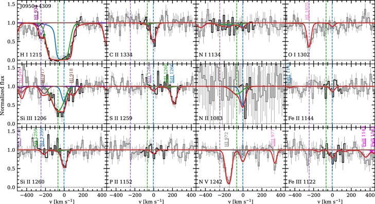
Figure 27. Fit to absorption lines at zabs = 0.01714 in the spectrum of J0950+4309. The synthetic profile is shown in red, and the contribution from each component, associated with the studied galaxy, is shown in green, blue, and purple (and orange). Dashed vertical lines represent the position of each component. Vertical sticks indicate the position of other absorption lines, associated with the MW (magenta sticks) and remote galaxies.
Download figure:
Standard image High-resolution image
Figure 28. Fit to absorption lines at zabs = 0.06013 in the spectrum of J1237+4447. Lines are the same as in Figure 27.
Download figure:
Standard image High-resolution image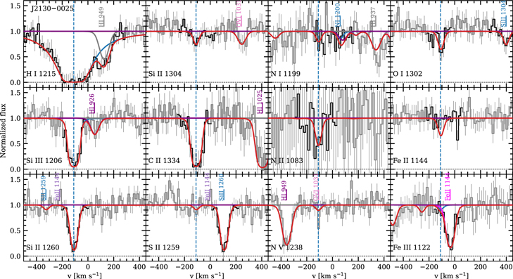
Figure 29. Fit to absorption lines at zabs = 0.01966 in the spectrum of J2130−0025. Lines are the same as in Figure 27.
Download figure:
Standard image High-resolution image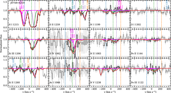
Figure 30. Fit to absorption lines at zabs = 0.03181 in the spectrum of J0758+4219. Lines are the same as in Figure 27.
Download figure:
Standard image High-resolution image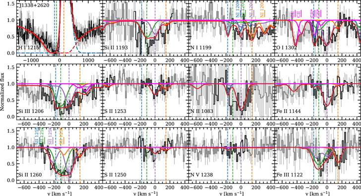
Figure 31. Fit to absorption lines at zabs = 0.02604 in the spectrum of J1338+2620. Lines are the same as in Figure 27.
Download figure:
Standard image High-resolution imageB.1. Comments to Fit to Absorption Systems
B.1.1. J0755+3911
We measured the H i and metal species column densities of the absorption system at the redshift of the AGN 1-71974 (zgal = 0.0336). The absorption system consists of at least four velocity components detected in H i Lyα and Si iii 1206 Å transitions. The H i absorption consists of two weak components with column densities ∼1012.8 and 1013.3 cm−2, which are blueshifted by −62 and −228 km s−1 with respect to the galaxy redshift. The Si iii 1206 absorption is detected in two components at −130 and −200 km s−1, which are shifted with respect to H i absorption lines. We fitted the absorption system with four velocity components with the redshifts tied to the redshift of the prominent H i and Si iii absorptions. The result of the fit is given in Table 5, and line profiles are shown in Figure 32.
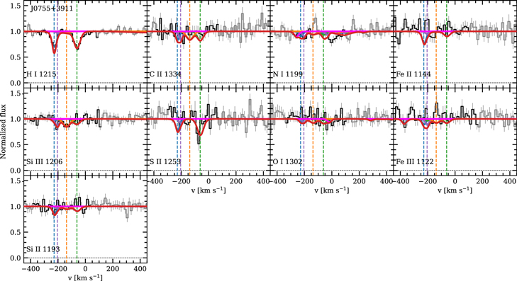
Figure 32. Fit to absorption lines at zabs = 0.03362 in the spectrum of J0755+3911. Lines are the same as in Figure 27.
Download figure:
Standard image High-resolution imageTable 5. Fit Results to Absorption Systems
| zabs | v | b |

| |||||||||||||
|---|---|---|---|---|---|---|---|---|---|---|---|---|---|---|---|---|
| (km s−1) | (km s−1) | (H i) | (Si ii) | (Si iii) | (C ii) | (S ii) | (S iv) | (N i) | (N ii) | (N v) | (O i) | (O vi) | (Fe ii) | (Fe iii) | (Ar i) | |
| J0755+3911, zem,corr = 0.03362 | ||||||||||||||||
| 0.03284 | −228 |

| <12.8 |

|

| <13.4 | <14.7 | N/C | <13.5 | N/C | N/C | <13.8 | N/C | <13.7 | <13.5 | N/C |
| 0.03292 | −203 |

| <13 | <12.7 |

| <13.4 | <14.0 | N/C | <13.3 | N/C | N/C | <13.1 | N/C | <13.7 | <13.5 | N/C |
| 0.03315 | −136 | <20 | <12.2 | <12.8 |

| <15 | <13.8 | N/C | <13.0 | N/C | N/C | <13.8 | N/C | <13.7 | <13.2 | N/C |
| 0.03342 | −62 |

|

| <12.7 | <12.6 | <13.6 | <14.5 | N/C | <13.7 | N/C | N/C | <13.5 | N/C | <13.9 | <13.5 | N/C |
| Total: |

|

|

|

| <15.0 | N/C |

| N/C | N/C |

| N/C |

| <13.5 | N/C | ||
| J0758+4219, zem,corr = 0.03181 | ||||||||||||||||
| 0.03138 | −115 |

|

|

|

| N/C | <14.4 | <14.5 | <13.8 | <14.3 | <13.6 | <14.0 | N/C | <13.7 | <14.0 | <14.0 |
| 0.03202 | 52 |

|

|

|

| N/C |

| <15.0 | <13.7 | <14.0 | <13.3 | <13.9 | N/C | <14.0 | <14.3 | <14.3 |
| 0.03226 | 130 |

|

|

|

| N/C |

| <15.0 | <13.6 | <14.1 | <13.3 | <13.9 | N/C | <13.8 | <14.4 | <14.3 |
| 0.03263 | 230 |

|

| N/A | <12.3 | N/C | N/A | N/A | N/A | N/A | N/A | N/C | N/A | N/A | N/A | N/A |
| Total: |

|

|

| N/C |

| <15.0 |

|

| <13.5 | <14.0 | N/C | <13.9 | <14.4 | <14.3 | ||
| J0838+2453(A), zem,corr = 0.02843 | ||||||||||||||||
| 0.02834 | −34 |

|

| <13.5 |

| N/C | <14.7 | N/C | <14.7 | N/A | N/A | <14.7 | N/A | <15.5 | N/A | N/A |
| 0.02812 | −93 | <20 | N/A |

|

| N/C | <15 | N/C | <13.6 | N/A | N/A | <14.5 | <14.1 | N/A | N/A | N/A |
| 0.02774 | −201 |

| N/A |

| <13.5 | N/C | 1 < 13.5 | N/A | <13.7 | N/A | N/A | <14.3 | N/A | N/A | N/A | N/A |
| Total: | −100 |

|

|

| N/C |

| N/A | <14.7 | N/A | N/A | <15 | N/A | <15 | N/A | N/A | |
| J0838+2453(B), zem,corr = 0.02843 | ||||||||||||||||
| 0.02584 | −754 |

|

|

|

| N/C |

| N/A | <13.7 | N/A | N/A | <13.0 | N/A | <16.0 | N/A | N/A |
| 0.02556 | −853 | <80 | N/A |

| <13.3 | N/C |

| N/A | <14.4 | N/A | N/A | <13.0 | N/A | N/A | N/A | N/A |
| Total: | −800 |

| <13.6 |

| N/C |

| N/A | <14.4 | N/A | N/A | <14.5 | N/A | N/A | N/A | N/A | |
| J0950+4309, zem,corr = 0.01714 | ||||||||||||||||
| 0.01713 | −2 |

|

|

|

|

| <14.7 | N/C | <14.3 | N/A | <13.8 | <14.0 | N/C | <14.3 | <14.0 | N/C |
| 0.01696 | −52 |

|

| <12.4 |

| <13.6 | <14.6 | N/C | <14.4 | <16.3 | <14.1 | <14.0 | N/C | <14.2 |

| N/C |
| 0.01630 | −247 | <100 |

| <12.7 | <12.7 | <14.1 | <14.6 | N/C | <14.0 | <16.0 | <13.5 | <14.6 | N/C | <14.0 | N/A | N/C |
| Total: |

|

|

|

|

| N/C |

| <16.2 |

|

| N/C |

|

| N/C | ||
| J1237+4447(A), zem,corr = 0.06013 | ||||||||||||||||
| 0.05960 | −151 |

|

| <13.0 |

|

|

| <14.3 | <13.3 | <13.5 |

| N/A | <14.3 | <13.8 | <13.8 | <13.4 |
| 0.05993 | −57 |

|

| <12.5 |

| <14.7 | <14.3 | <14.1 | <13.4 | <13.8 | <13.2 | N/C | <15.3 |

| <14.0 | <13.3 |
| 0.06119 | 302 |

|

| N/A | <12 | N/A | N/A | N/A | N/A | N/A | N/A | N/C | N/A | N/A | N/A | N/A |
| Total: |

| <13 |

| <14.7 |

| <14.2 |

| <13.5 |

| N/C | <14.3 |

| <11.0 | <13.5 | ||
| J1237+4447(B), zem,corr = 0.06013 | ||||||||||||||||
| 0.05960 | −151 |

|

| <13.0 |

|

|

| <14.3 | <13.3 | <13.5 |

| N/A | <14.3 | <13.8 | <13.8 | <13.4 |
| 0.05993 | −57 |

|

| <12.6 |

| <14.8 | <14.2 | <14.1 | <13.3 | <13.6 | <13.2 | N/C |

|

| <14.2 | <13.2 |
| 0.06119 | 302 |

|

| N/A | <12 | N/A | N/A | N/A | N/A | N/A | N/A | N/C | N/A | N/A | N/A | N/A |
| Total: |

|

|

|

|

| <13.9 |

| <13.5 |

| N/C |

|

| <11.0 | <13.2 | ||
| J1338+0311, zem,corr = 0.02604 | ||||||||||||||||
| 0.02543 | −178 |

| N/A |

|

| N/C |

| N/C |

|

|

| <15.0 | N/C |

|

| N/A |
| 0.02566 | −110 |

| N/A |

|

| N/C |

| N/C |

|

|

|

| N/C |

| N/A | N/A |
| 0.02603 | 2 |

|

|

|

| N/C |

| N/C |

|

|

|

| N/C |

| <14.6 | N/A |
| 0.02639 | 146 |

| N/A |

|

| N/C |

| N/C |

|

| <12 |

| N/C | <14.0 | <14 | N/A |
| Total: |

|

|

| N/C |

| N/C | <14.3 | <16 | <13.8 |

| N/C | <14.6 | <14.3 | N/A | ||
| J2106+0909, zem,corr = 0.0437 | ||||||||||||||||
| 0.04423 | 135 |

|

| <13.0 | <13.2 | N/C | <14.8 | N/A | N/A | N/A | N/A | N/A | N/A | N/A | N/A | N/A |
| J2130−0025, zem,corr = 0.0200 | ||||||||||||||||
| 0.01967 | −146 |

|

|

|

|

| <14.6 | N/C |

| <14.7 | <13.7 |

| N/C |

| <11 | N/A |
B.1.2. J0758+4219
We detected the absorption system associated with the CGM of galaxy 1-44487, which consists of four velocity components detected in H i, Si ii, Si iii, and S ii absorption lines. The velocity components of metal absorption lines correspond well with the position of the H i velocity components. Therefore, we fitted this system with four components. One of the H i components is blended with the MW S ii 1253 Å absorption line, and we fitted the MW S ii absorptions consistently with the fit to the galactic absorption lines. The result of the fit is given in Table 5, and line profiles are shown in Figure 30.
B.1.3. J0838+2453
In the spectrum of the AGN J0838+2453, we detected two H i absorptions at −34 and −750 km s−1 with respect to the redshift of the host galaxy. Because of the low S/N for this spectrum, the associated metal absorption lines are detected only in Si iii 1206 Å transition, which is located close to the H i Lyα quasar emission line. The Si iii absorption has five velocity components. Two velocity components correspond well with the position of the H i absorption components, whereas other three component are detected only in Si iii. Therefore, we fitted the absorption system with five velocity components. The result of the fit is given in Table 5, and line profiles are shown in Figure 33.
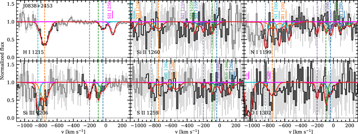
Figure 33. Fit to absorption lines at zabs = 0.02843 in the spectrum of J0838+2453. Lines are the same as in Figure 27.
Download figure:
Standard image High-resolution imageB.1.4. J0950+4309
The absorption system at the redshift of the galaxy 1-166736 is well detected in H i, Si ii, Si iii, and C ii transitions. The H i absorption line is saturated; therefore, we derived the velocity structure from the fit to metal absorption lines. We found that Si ii and C ii absorptions can be well fitted by one component that is redshifted relative to the center of the strong Si iii absorption line. The additional blue component seen in only the Si iii absorption line also has a higher Doppler parameter, which indicates the difference in physical conditions between two components. The redshift of the blue component has been chosen to well fit the blue wing of H i Lyα absorption. Additionally, we detected the third weak component at −247 km s−1 with respect to the galactic redshift, which is detected only in the H i profile. The result of the fit is given in Table 5, and line profiles are shown in Figure 27.
B.1.5. J1237+4447
The absorption system at the redshift of the galaxy is detected in H i Lyα and Lyβ and Si iii absorption lines. The Si ii absorption line is blended by the saturated C ii and C ii* absorption lines of the MW. Since the H i Lyα is saturated, we derived the velocity structure from the fit to Si iii absorption line, which is well fitted by two velocity components. The fit to the redshifted component in the H i line profile is degenerate in the parameter space N(H I) − b and has two solutions with low and high N(H I). We consider both solutions they name: case A and case B. The likelihood functions are shown in Figure 17. The result of the fit is given in Table 5, and line profiles are shown in Figure 28.
B.1.6. J1338+0311
The absorption system associated with the host galaxy of the AGN 12-192116 has strong damped H i Lyα absorption (N = 1020.2 cm−2). We described the fit to the H i Lyα line in Section 2.2.2. The associated metal absorption lines are fitted by four velocity components. The result of the fit is given in Table 5, and line profiles are shown in Figure 31.
Table 6. Fit Results to cloudy Photoionization Model of Absorption Systems
| Quasar | zabs | v |

|

| [X/H] |

|

| F* |
|---|---|---|---|---|---|---|---|---|
| (km s−1) | (cm−2) | (cm−2) | (Drain/cm−3) | |||||
| J0755+3911 | Average: |

|

|

|

|

|

| |
| J0758+4219 | 0.03138 | −115 |

|

|

|

|

| <1 |
| 0.03202 | 52 |

|

|

|

|

|

| |
| 0.03226 | 130 |

|

|

|

|

|

| |
| 0.03261 | 230 | N/A | N/A | N/A | N/A | N/A | N/A | |
| Average: |

|

|

|

|

|

| ||
| J0838+2453 | Average(A): |

|

|

|

|

|

| |
| Average(B): |

|

|

|

|

| <1 | ||
| J0950+4309 | 0.01713 | −2 |

|

|

|

|

|

|
| 0.01696 | −52 |

|

|

|

|

|

| |
| 0.01630 | −247 | N/A | N/A | N/A | N/A | N/A | N/A | |
| Average: |

|

|

|

|

|

| ||
| J1237+4447 | 0.05960 | −151 |

|

|

|

|

| <1 |
| 0.05993(A) | −57 |

|

|

|

|

|

| |
| 0.05993(B) | −57 |

|

|

|

|

|

| |
| 0.06119 | 302 | N/A | N/A | N/A | N/A | N/A | N/A | |
| Average(A): |

|

|

|

|

|

| ||
| Average(B): |

|

|

|

|

|

| ||
| J1338+0311 | Average: |

|

|

|

|

| ||
| J2106+0909 | 0.04423 | 135 | N/A | N/A | N/A | N/A | N/A | N/A |
| J2130−0025 | 0.01967 | −110 |

|

|

|

|

|

|
Download table as: ASCIITypeset image
B.1.7. J2106+0909
We detected only one weak absorption line of H i Lyα (N = 1013.7 cm−2) at the redshift of galaxy 1-113242. The associated Si iii absorption line is blended with the MW S ii absorption lines; therefore, we can set only an upper limit to the Si iii column density. The result of the fit is given in Table 5, and line profiles are shown in Figure 34.
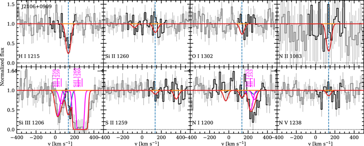
Figure 34. Fit to absorption lines at zabs = 0.04375 in the spectrum of J2106+0909. Lines are the same as in Figure 27.
Download figure:
Standard image High-resolution image
Figure 35. The cases of nondetections. The absorption lines of H i, Si iii, Si ii, and N v in the HST COS spectra of J1653+3945, J1709+3421, and J1629+4007 at the redshifts of the corresponding galaxies (1-594755, 1-561034, and 1-564490, respectively) are shown. The synthetic profile is depicted in red. The dashed vertical line represents the likely position of the absorption system. Vertical sticks indicate the position of absorption lines, associated with the Milky Way (MW; magenta sticks) and remote galaxies.
Download figure:
Standard image High-resolution imageB.1.8. J2130-0025
We detected strong saturated absorption lines of H i and metal species at the redshift of galaxy 1-180522. The absorption lines are well fitted with one-component model. The result of the fit is given in Table 5, and line profiles are shown in Figure 29.
B.1.9. Nondetection
In three cases (J1653+3945, J1709+3421 and J1629+4007), we do not detect any absorption (in H i or any of the metal ions) within the range of  km s
km s relative to the galaxy redshifts (1-594755, 1-561034, 1-564490). Figure 36 shows the parts of quasar spectra near the expected positions of HI, SiII, SiIII, NV lines. We set upper limits on N(HI)
 cm
cm .
.
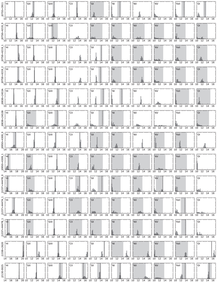
Figure 36. The fit results to measured species column densities in our sample with cloudy simulation. Dashed vertical lines and light shaded areas represent the most probable value and its uncertainty. The light shaded area without lines represent the upper limit. The histograms show the distributions of species column densities in cloudy simulation.
Download figure:
Standard image High-resolution image
Footnotes
- 10
The estimate corresponds to a 3σ upper limit of the H i mass surface density for nondetections; see Masters et al. (2019).
- 11
In the case of the quasar–galaxy pair J1629+4007-1-564490, there is another galaxy (SDSS J162842.25+400726.1) that is closer to the quasar sight line than the targeted MaNGA galaxy, but it has a higher redshift z = 0.03357 versus z = 0.02588. For this quasar sight line, we detect a weak H i absorption at redshift z = 0.033, associated with the SDSS J162842.25+400726.1 galaxy, and do not detect any absorption within ±1000 km s−1 at the redshift of MaNGA galaxy 1-564490.
- 12
- 13
The COS LSF has broad non-Gaussian wings, and the shape varies with the wavelength. We used the approximation by the piecewise function taken from the COS documentation; see, e.g., https://www.stsci.edu/hst/instrumentation/cos/performance/spectral-resolution.
- 14
The Lyβ H i line is covered by HST spectra for only one galaxy, 1-575668, which has a higher redshift zgal ≃ 0.06 than others.
- 15
- 16
We used the UVB model Q18 recommended by Khaire & Srianand (2019) as a fiducial.
- 17
The impact parameter denotes the lower limit to the distance between the galactic center and the absorption system along the quasar sight line. The real distance can be higher; however, it is believed that the distribution of gas around galaxies strongly decreases with the distance, and therefore the impact parameter has the highest probability of gas detection.
- 18
The impact parameter can be presented in proper (physical) kiloparsecs by multiplying the angular separation (in arcseconds) by the angular diameter distance (DA ), and in comoving kiloparsecs (ckpc) by multiplying the angular separation by the comoving distance (DM ), which is larger than DA by a factor of (1 + z).
- 19
In Péroux et al. (2020), the angle ϕ is referred to as the "azimuthal angle," but we reserve that term for the disk in-plane angle with respect to the major axis.
- 20
The galactic redshift was corrected for the systematic velocity offset Vsys derived by fitting to MaNGA maps; see Section 2.3.2.