


Abstract
Simulated galaxy distributions are suitable for developing filament detection algorithms. However, samples of observed galaxies, being of limited size, cause difficulties that lead to a discontinuous distribution of filaments. We created a new galaxy filament catalog composed of a continuous cosmic web with no lone filaments. The core of our approach is a ridge filter used within the framework of image analysis. We considered galaxies from the HyperLeda database with redshifts 0.02 ≤ z ≤ 0.1, and in the solid angle 120° ≤ R.A. ≤ 240°, 0° ≤ decl. ≤ 60°. We divided the sample into 16 two-dimensional celestial projections with redshift bin Δz = 0.005, and compared our continuous filament network with a similar recent catalog covering the same region of the sky. We tested our catalog on two application scenarios. First, we compared the distributions of the distances to the nearest filament of various astrophysical sources (Seyfert galaxies and other active galactic nuclei, radio galaxies, low-surface-brightness galaxies, and dwarf galaxies), and found that all source types trace the filaments well, with no systematic differences. Next, among the HyperLeda galaxies, we investigated the dependence of the g − r color distribution on the distance to the nearest filament, and confirmed that early-type galaxies are located on average further from the filaments than late-type ones.
Export citation and abstract BibTeX RIS

Original content from this work may be used under the terms of the Creative Commons Attribution 4.0 licence. Any further distribution of this work must maintain attribution to the author(s) and the title of the work, journal citation and DOI.
1. Introduction
1.1. Cosmic Web
The notion of a cellular large-scale structure (LSS; de Lapparent et al. 1986) of the universe has long been recognized as an important component of the astronomical picture of the world (Bernardeau et al. 2002). Optical radiation, coming from the stellar content of a galaxy, is the most accessible for observations, but a much larger mass is concentrated in dark matter (DM), whose distribution can be detected by galactic flows (Courtois et al. 2013), gravitational lensing (Kaiser & Squires 1993), X-ray radiation of clusters (Reiprich & Böhringer 2002), via the Sunyaev-Zeldovich effect (Sunyaev & Zeldovich 1980), and other methods (Shulga et al. 2014). The spatial structure of the cosmic web is reflected primarily in needle-like filaments. Clusters of galaxies occupy a small volume, voids contain a small number of galaxies, and walls contain a number of filaments (van de Weygaert & Schaap 2009; Cautun et al. 2013). Through the structure of the cosmic web one can determine the properties of DM (Alexander et al. 2022) and the expansion laws of the universe, or validate the theory of inflation (Springel et al. 2006). The localization of voids (Mao et al. 2017; Peper et al. 2023) can aid cosmological tests (Paz et al. 2023) and the study of the few galaxies that occupy them (Porter et al. 2023).
Two principles lie at the heart of the LSS theory: (i) the hypothesis of the Gaussian distribution of initial density perturbations, and (ii) Zeldovich's approximation within which one can describe their evolution (van de Weygaert 2002). Most of the methods for describing the LSS have been tested via numerical simulations (Libeskind et al. 2018; Ganeshaiah Veena et al. 2019; Bonnaire et al. 2020; Banfi et al. 2021; Zhang et al. 2022), and only a few have been applied to actual observational surveys (Sousbie 2011; Sousbie et al. 2011; Tempel et al. 2014; Chen et al. 2016; Carrón Duque et al. 2022). A detailed comparison of several modern methods of filament detection is given by Libeskind et al. (2018).
A common method for detecting cosmic structures in surveys like the Sloan Digital Sky Survey (SDSS; York et al. 2000; Abazajian et al. 2009) is a topological method called Discrete Persistent Source Extractor (DisPerSE, Sousbie 2011; Sousbie et al. 2011), based on the Delaunay tesselation of the discrete sample of points symbolizing galaxies, which allows one to extract filaments, walls, and voids. DisPerSE was applied to illustrate the effect of modified theories of gravity on the length, mass, and thickness of filaments (Ho et al. 2018). A method of approximating the distribution of galaxies with cylinders (the Bisous model; Stoica et al. 2010) was used by Tempel et al. (2014) and Muru & Tempel (2021). As a result, the galaxies were grouped into small cylinders (with at least three galaxies inside each cylinder) and were combined into a larger filament net. It was confirmed that about 40 per cent of the mass is gathered in the filaments (Forero-Romero et al. 2009; Jasche et al. 2010), while occupying only 8 per cent of the volume. The detection of filaments was also performed by Chen et al. (2016) and Carrón Duque et al. (2022) in redshift layers with radial thicknesses of about 20 Mpc. This approach allows to compensate for the effect of peculiar velocities of galaxies in local gravitational fields by solving a simplified two-dimensional problem, mitigate redshift-space distortions, correlate the projections with maps of the cosmic microwave background, trace the evolution of the LSS throughout cosmic time, etc. One particular disadvantage is the insensitivity to filaments oriented close to the line of sight and inaccurate detections regarding filaments spanning a few neighboring redshift layers, but the choice of the thickness of the redshift layers is expected to balance the biases and errors. Chen et al. (2016) used a variant of a ridge filter applied directly to data, and obtained a filament net within 0.05 < z < 0.7, whereas Carrón Duque et al. (2022) extended the sample to redshifts up to z = 2.2 and employed spherical coordinates to bypass projection effects. The resulting nets are consistent with the local overdensities of the cosmic web, but both works also contain some lone, very short filaments that are not connected to the rest of the network and are not obviously associated to any bigger structure, as well as gaps in the overall network.
The ambiguities of different algorithms and observational restrictions urge the development of more careful methods for detecting and connecting filaments. A way to perform general statistical analyses of the LSS is to generate the apparent distribution of galaxies assuming a certain matter density field (Voitsekhovski & Tugay 2018). This will determine the overall statistical characteristics of the filaments and therefore describe the LSS of the universe as a whole. It also allows to produce mock data sets with statistical properties matching those of actual observational surveys. Nowadays, only the closest affiliates of the Local Supercluster (Kim et al. 2016; Castignani et al. 2022), which are associated with the accumulation of Virgo galaxies, are most prominently identified.
1.2. Color and Distance Distributions
Early galaxy color studies were based on the development and implementation of different photometric systems with appropriate photometric stellar standards 3 (de Vaucouleurs 1961; Sandage & Visvanathan 1978; Fukugita et al. 1995). Detailed color studies were conducted for early-type (elliptical) galaxies (Bernardi et al. 2003, 2005), as well as for late-type (spiral) galaxies (Tully et al. 1982; Peletier & de Grijs 1998; Fraser-McKelvie et al. 2016).
Galaxy color distributions are commonly explained by a halo model that links the galaxy color to the mass of the DM halo (Skibba & Sheth 2009; Hearin & Watson 2013). Colors are also correlated with luminosities and morphological types of the galaxies (Kodama & Arimoto 1997; Kodama et al. 1998). Such relations were analyzed by Mobasher et al. (1986) and Bower et al. (1992a, 1992b) for nearby galaxies in the Virgo and Coma clusters, and by Lange et al. (2015) for more distant galaxies at z < 0.1. An important feature of galaxy colors is a bimodal distribution that relates to spiral and elliptical galaxies (Strateva et al. 2001). This is clearly seen in the SDSS (Baldry et al. 2004) and Millenium Galaxy Catalog (Driver et al. 2006), as well as for distant galaxies at z < 2.5 (Brammer et al. 2009). Bimodality was also found in the two-dimensional color–color distribution (Park & Choi 2005). The bimodal character appears in cosmological computer simulations as well, e.g., Illustris (Nelson et al. 2018), or Evolution and Assembly of GaLaxies and their Environment (Trayford et al. 2015). Colors are connected with environment, in dependence on the surface brightness and luminosity (Blanton et al. 2005). The existence of the green valley, though, has been challenged (Eales et al. 2018), and explained to arise as a consequence of the Malmquist bias in the submillimeter wave band.
Redder and more massive galaxies are located closer to filaments (Luber et al. 2019). The surplus of massive red elliptical galaxies in the SDSS filaments was analyzed by Kuutma et al. (2017, 2020), and Welker et al. (2020) presented similar results for the Sydney Australian Astronomical Observatory Multi-object Integral field spectrograph galaxy survey and determined the angles between the galaxies' spins and filaments. A corresponding study of the orientation of X-ray clusters in relation to the filaments was performed by Shevchenko & Tugay (2017).
1.3. Outline
We present the results of applying a ridge filter within the framework of image analysis to build a continuous net of filaments for radial layers of the galaxy distributions up to redshift z = 0.1 within a 120° × 60° solid angle. This paper is organized as follows. Section 2 gives a description of the utilized galaxy sample and discusses its completeness. In Section 3 the algorithm for filament detection is outlined. In Section 4 we test our approach on a simulated data set. In Section 5 we provide a comparison of our filaments with similar outcomes by Chen et al. (2016). Section 6 is devoted to validating the extracted filament net through applications: a statistical analysis of distances of various astronomical sources to the nearest filament is performed in Section 6.1, and in Section 6.2 we examine how the g − r color of galaxies changes with the distance from the nearest filament. The discussion and concluding remarks are gathered in Section 7. We utilize the cosmological parameters H0 = 70 km s−1 Mpc−1 and Ω = 0.32 throughout.
2. Sample
We selected the SDSS region by restricting the coordinates within 120° ≤ R.A. ≤ 240°, 0° ≤ decl. ≤ 60°. The data were taken from the HyperLeda database 4 of extragalactic objects (Makarov et al. 2014). We selected radial redshift layers with thickness Δz = 0.005, which corresponds to 20 Mpc. Such thickness was selected in order to perform a direct comparison with the previous results of Chen et al. (2016; see Section 5).
Extragalactic voids have diameters ranging from 50 to 100 Mpc, so one should find a number of voids spanning a few neighboring layers. We selected all HyperLeda objects with appropriate coordinates and redshifts to get the largest possible data set for filament detection. We found that the number N(z) of galaxies in a redshift layer 5 starts to decrease slightly at z ≳ 0.08 (Figure 1(a)). We conclude that regions at z > 0.1 may not be appropriate for a correct filament detection with the sample at hand, especially given the potential for a growing incompleteness of any data set at larger redshifts. Nevertheless, Chen et al. (2016) and other authors (Sousbie et al. 2011; Tempel et al. 2014; Malavasi et al. 2017; Carrón Duque et al. 2022) presented some results of filament detection at much larger distances.

Figure 1. (a) Number of galaxies N(z) in each redshift bin. (b) The slope of the linear regression of the number of galaxies N( ≤ z) up to redshift z in a log–log plot gives the exponent α, which is then used (c) to demonstrate the catalog redshift completeness in the range 0.02 ≤ z ≤ 0.1. The horizontal line illustrates that N( ≤ z)/zα
is constant in this range. The error bars in panels (a) and (b),  , are about the size of the graphed points and are taken into account in the calculations.
Download figure:
Standard image High-resolution imageIf galaxies were distributed randomly and uniformly, their cumulative number N(≤ z) should increase proportionally to zα with α = 3. Due to their clustering in filaments, the power-law index α differs from 3, but should remain constant for z up to some redshift completeness limit. We therefore construct N(≤ z), approximate it by a power law, and determine α (Figure 1(b)). Then we examine the ratio N(≤ z)/zα , which compares the actual number of galaxies in the sample and that of the power-law approximation (up to the constant of proportionality). We observe that the ratio is constant over a range of redshifts (Figure 1(c)); hence we conclude that the considered catalog is consistent with being complete up to z = 0.1.
The deviation at z < 0.02 is due to the domination of local, point-like structures (compared to the cosmic web observed at redshifts z > 0.02). Point-like structures are single galaxies and clusters that dominate the most local universe causing a deviation from the N(≤ z) ∝ zα law. The first three radial layers correspond to the Local Supercluster and its boundaries (in particular, many dwarf galaxies in the Local Group at z < 0.01). We live in the Local Galaxy Supercluster, which is a major overdensity in the galaxy distribution at ∼100 Mpc scales. Our Supercluster is surrounded by thin filaments and voids. The central object of the Local Supercluster, the Virgo galaxy cluster, is located at z = 0.004, which is below the minimal redshift of our sample. There are five known filaments in the Local Supercluster (Kim et al. 2016), and only one of them falls within our 120° × 60° field of view. Hence we do not detect significant one-dimensional structures at this scale. The second supercluster, Coma, is separated from us by the Local Void. The Coma cluster, a central object of the corresponding supercluster, lies in the redshift bin z ∈ [0.02, 0.025]. At this scale, a more uniform cosmic web emerges. In summary, our filament extraction algorithm yielded biased outcomes for z < 0.02, resulting in a number of apparently spurious detections. Eventually, we analyzed 16 equally sized, nonoverlapping redshift bins in the range 0.02 ≤ z ≤ 0.1.
The physical extent  , measured in Mpc, of the structures spanning a given angular size θ on the sky
6
(i.e., a projection onto the celestial sphere) depends on the redshift z as
, measured in Mpc, of the structures spanning a given angular size θ on the sky
6
(i.e., a projection onto the celestial sphere) depends on the redshift z as

where  is the proper distance, with
  , and θ is measured in degrees. This implies that the scale of detected filaments increases with the redshift as well. For instance, the angular length of a
  Mpc filament (idealized to be perpendicular to the line of sight) is θ = 6
 6 at z = 0.02, whereas it is θ = 12 at z = 0.1. In other words, the 120° × 60° solid angle considered corresponds to a 180 Mpc × 90 Mpc patch at z = 0.02, and a 960 Mpc × 480 Mpc patch at z = 0.1.
3. Method
The core of the filament extraction algorithm is the application of a ridge filter (Steger 1998; Damon 1999; Lopez-Molina et al. 2015) directly on images of the celestial distribution of galaxies in the Mollweide projection. The functionality of Mathematica's built-in command RidgeFilter 7 is exploited for this purpose. A ridge is, simply put, a long and narrow edge of an elevation (the term corresponding to mountain ridges). In other words, a ridge can be identified if a two-dimensional function has a small second-order directional derivative in one direction (along the ridge) and a large derivative in the other direction (perpendicular to the ridge).
The image function f(x, y) at pixel position (x,y) is convolved with a symmetric Gaussian kernel,

with a set value of σ (chosen hereinafter to be σ = 30 pixels; see Appendix C), producing a response h(x, y). The second-order structure characterizing ridges can be captured with the Hessian matrix, H , of the function h. The ridges are regions with major eigenvalues of H that are large compared to the minor eigenvalues. In particular, one is interested in computing the main principal curvature at each pixel of the image through the main negative eigenvalue of H (Lindeberg 1998).
The crucial steps of the whole procedure are illustrated in Figure 2. The ridge filter is applied to an 1800 px × 900 px image of galaxy locations (Figure 2(a)). The exact dimensions of the image are not that important, as in the next steps the image will be blurred and morphologically transformed. In general, the image needs to be of sufficient resolution for the crucial details to be discernible, with σ appropriately adjusted. We take the distortion of a projection of a spherical sector onto a plane into account by appropriately squeezing such Cartesian projection at higher latitudes, therefore sustaining the proper geometry as much as possible. The smaller the considered patch of the sky, the less distorted the geometry.

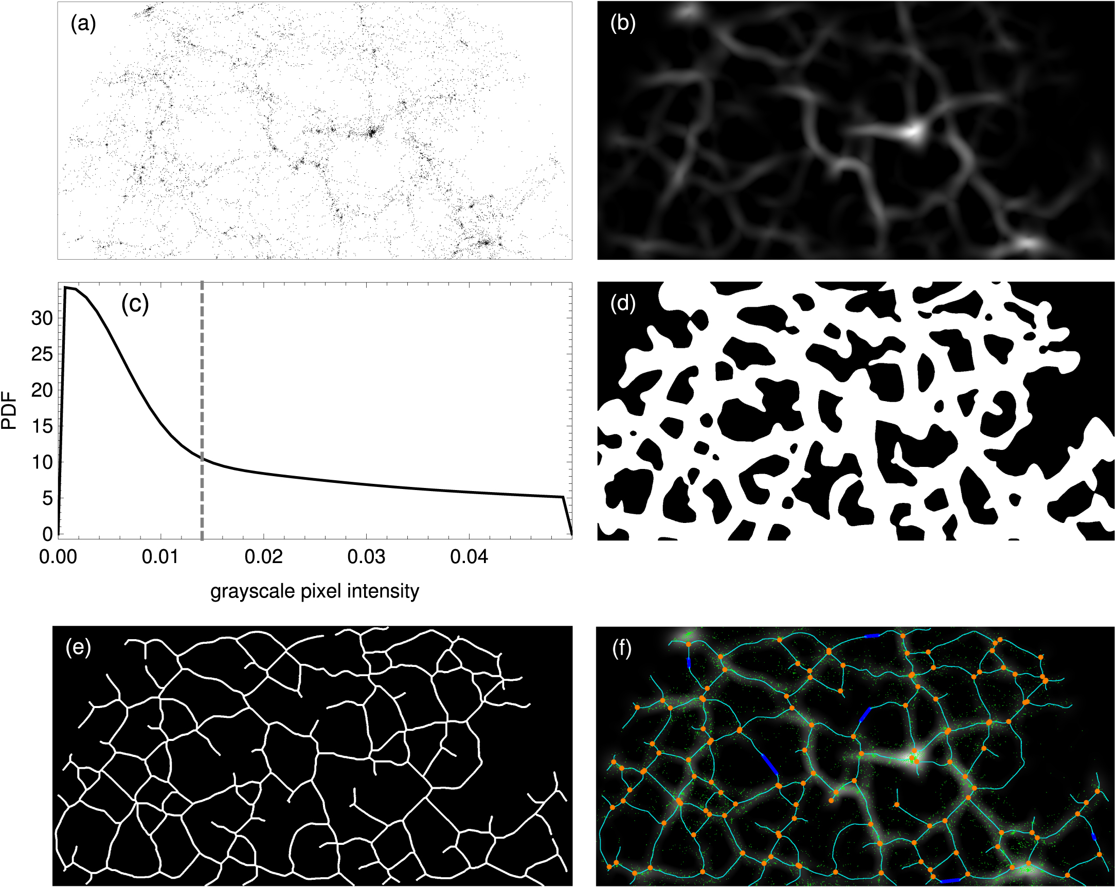
Figure 2. Scheme of the filament extraction algorithm for the redshift bin z ∈ [0.025, 0.030]. (a) Celestial distribution of galaxies in the 120° × 60° field of view. Note that the projection at higher latitudes is appropriately squeezed to account for the distortion when projecting a spherical sector onto a plane, which is necessary for the subsequent steps of the image analysis. (b) Direct application of the RidgeFilter yields a grayscale density map, where brighter regions correspond to higher densities. (c) To decide in a binary manner which parts of panel (b) should be associated with filaments, a smooth kernel density of the grayscale pixel intensity is constructed, and the threshold for the separation is chosen as the pixel intensity at which a knee in the probability density function (PDF) is present (marked herein with a vertical dashed line). (d) Pixel intensities exceeding the threshold are colored white (related with overdensities associated with filaments), whereas voids are colored black. (e) A morphological thinning of the binary plot in panel (d) results in the skeleton network of the filamentary LSS. (f) The last step is to connect the tails with other tails via great arcs if they point at each other within a 45° cone (blue lines). Orange dots denote the filament intersections, small green dots mark the location of the galaxies from panel (a), and the grayscale image in the background is the gradient from panel (b).
Download figure:
Standard image High-resolution imageThe RidgeFilter produces a smoothed grayscale image with pixel intensities corresponding to the densities of the galaxy distributions (color coded according to their pixel intensity values: 0 for black = low density, and 1 for white = high density; Figure 2(b)). To choose the threshold for the pixel intensity to decide which areas of this grayscale image harbor filaments (i.e., which have densities high enough to be associated with a filament), the smooth kernel distribution of the pixel intensities of the whole image is constructed with Silverman's rule (Silverman 1986, Figure 2(c)), and the threshold is defined to be the value where the distribution has a knee point, i.e., its curvature is maximal (Satopää et al. 2011), marked by the vertical dashed line in Figure 2(c). Values above this threshold mark the filaments, and values below this threshold mark the voids. This step yields a binary image with separated regions containing the filamentary surroundings and voids (Figure 2(d), marked with white and black, respectively). Small, isolated filaments (i.e., those with less than 104 pixels) are deemed artifacts and are removed using the Delete-SmallComponents 8 command; likewise very small voids are closed, i.e., the surrounding filamentary structures are expanded to absorb the voids using the Closing 9 command. Finally, the filamentary regions are morphologically squeezed (thinned) with the Thinning 10 command to form a net of interconnected one-dimensional filaments (Figure 2(e)).
At this stage the net still contains some artifacts, like tails, i.e., filaments with one loose end, and pairs of tails pointing at each other but not connected. Tails can be of physical meaning if they are longer than  Mpc—shorter ones are removed (with the use of the Pruning
11
command and based on the sizes computed via Equation (1)). By physical meaning we understand either tails pointing in the direction of the edge of the field of view, or tails protruding into the voids. The latter can indicate real filaments, whose parts might be obscured by the environment or observational constraints. It might also be possible that parts of the filaments have a deficit of bright galaxies, but still contain a significant amount of DM. We therefore keep such tails in the final net. Pairs of tails that point at each other within a 45° cone are connected with great arcs. From the resulting final net (Figure 2(f)), the locations of the filaments (cyan and blue lines in Figure 2(f)) and intersections (orange points in Figure 2(f)) are recorded, and constitute our filament catalog (Appendix A). In Figure 3 the distributions of the distance
Mpc—shorter ones are removed (with the use of the Pruning
11
command and based on the sizes computed via Equation (1)). By physical meaning we understand either tails pointing in the direction of the edge of the field of view, or tails protruding into the voids. The latter can indicate real filaments, whose parts might be obscured by the environment or observational constraints. It might also be possible that parts of the filaments have a deficit of bright galaxies, but still contain a significant amount of DM. We therefore keep such tails in the final net. Pairs of tails that point at each other within a 45° cone are connected with great arcs. From the resulting final net (Figure 2(f)), the locations of the filaments (cyan and blue lines in Figure 2(f)) and intersections (orange points in Figure 2(f)) are recorded, and constitute our filament catalog (Appendix A). In Figure 3 the distributions of the distance  to the nearest filament are displayed for each redshift bin separately. For higher redshifts the peak of the distribution shifts toward greater distances
  , and the distributions become flatter. This illustrates that at higher redshifts the observational biases start to play a role in analyzing the LSS.

Figure 3. Distributions of the distance from each HyperLeda galaxy to the nearest filament. The inset shows that lower curves consistently correspond to higher redshifts (according to the direction of the arrow). Colors are used only to distinguish between the curves.
Download figure:
Standard image High-resolution imageWe emphasize that, despite being based on the ridge formalism via the Hessian matrix approach (Libeskind et al. 2018; Rost et al. 2020), like several other works, a novelty in our overall procedure is to employ the ridge formalism to produce the grayscale images depicting the local galaxy densities, and then proceed exclusively with image analysis techniques that are topological in nature (Vandaele et al. 2020) to distort, transform, cleanse, and eventually extract the backbone of the filament network. Our overall goal was to produce a filament network that is as connected as possible, mitigating the fractured nets commonly obtained by other filament finders. We work on images of the Mollweide projection, which is an equal-area map.
The above described procedure was applied to all 16 redshift bins, producing a continuous filament network. The filament catalog is provided as an ancillary file (Appendix A), and a Mathematica notebook with the whole implementation (Appendix B) applied to mock data (see Section 4) is available from DOI:10.5281/zenodo.7971833. We briefly discuss the potential for a three-dimensional generalization of the algorithm within the image analysis framework in Section 7.2.
4. Test on Mock Data
We tested our algorithm with a random galaxy distribution. We used a sample of randomly distributed galaxies according to Voitsekhovski & Tugay (2018). The sample is generated by randomly distributing clusters (the average distance between them is denoted with 〈r〉), connected by filaments if the distance r satisfies A/2〈r〉 < r < 2A〈r〉, with A ∼ 1. The number of galaxies in a cluster is set to  , where nfilam is the number of filaments connected to a cluster. The size of a cluster is given by θ
D, where D = 14 and
, where nfilam is the number of filaments connected to a cluster. The size of a cluster is given by θ
D, where D = 14 and  is drawn from a uniform distribution. A small number of uniformly distributed isolated galaxies was also generated. The precise parameters of distributions were chosen to fulfill the condition of equality of two-point angular correlation function (2pACF) for the generated sample and the real distribution of galaxies from SDSS. The result of the filament extraction algorithm from Section 3, applied to this mock data set, is shown in Figures 4(a)–(b). Note that these plots, and similar subsequent ones, are displayed in Cartesian coordinates for ease of presentation, contrary to the algorithm itself, which relies on properly distorted projections (see Section 3 and Figure 2). Figure 4(c) displays in red the distribution of pixel values (in the grayscale color-coded density plot, i.e., the step depicted in Figure 2(b) that illustrates the procedure) at the particular galaxy positions. Shown in blue is the distribution obtained at the locations of the filament network extracted with the algorithm from Section 3. Compared to the pixel intensity distribution of a random sample of 104 points, uniformly distributed on the 120° × 60° spherical shell (plotted in green), these two distributions are similar in shape, which means that our filaments trace the LSS well, but the distribution of filaments (i.e., blue line) is statistically significantly shifted toward higher intensity values, i.e., corresponds to higher densities of galaxies than the mock data (i.e., red line). This is expected as filaments are regions of above-average (projected) number density. We therefore conclude that quantitatively the underlying filamentary structure is recovered with satisfying accuracy.

Figure 4. Simulated mock LSS. The parameters of random distributions were selected so that the 2pACF corresponds to that of an SDSS layer at a distance of 100 Mpc. (a) Initial points, generated as described in Section 4, overlaid on the corresponding density plot. The (logarithmic) color scale depicts the local concentration of points in arbitrary units (a.u.). (b) Resulting filament network of the final mock data set, obtained with our algorithm described in Section 3. The meaning of colors is the same as in Figure 2(f). Note that this plot, and similar subsequent ones, are displayed in Cartesian coordinates for ease of presentation, contrary to the algorithm itself, which relies on properly distorted projections (see Section 3 and Figure 2). (c) Histograms of the pixel intensities, extracted from the grayscale image of the density plot of the mock data (see the relevant step of the procedure illustrated in Figure 2(b)). The red (short-dashed) line shows the distribution of pixel intensities at the locations of the galaxies forming the mock sample. The blue (solid) line is the distribution extracted at the locations of the filament network from panel (b). This distribution is shifted toward values corresponding to higher densities, as it should be expected, as filaments are regions of galaxy overdensities. For comparison, the green (long-dashed) line is formed from the intensities of a random sample of uniformly distributed points.
Download figure:
Standard image High-resolution image5. Comparison with the Filament Catalog of Chen et al. (2016)
To compare our filament net with that of Chen et al. (2016), we employ the box-counting method designed as follows. We divide the 120° × 60° field of view into boxes at a constant step of 2° in the latitudinal direction, and an appropriate size in the longitudinal one. We choose the latter so that each box has approximately the same angular area, and start with 2° × 2° boxes at the equatorial strip (i.e., 60 boxes at this first strip), ending with 31 boxes at the last strip. We record the number of cells containing (i) both our and Chen et al. (2016)'s filaments, (ii) only Chen et al. (2016)'s filaments, and (iii) only our filaments (color coded with green, orange, and yellow, respectively, in Figure 5). That is, (i) the same filaments identified by both works, (ii) likely short, detached, spurious filaments, and (iii) regions filled in with filaments to maintain the continuity of the net. We find that both filament catalogs overlap in about 50% of the cases (i.e., about 50% of the boxes are filled by filaments from both catalogs; Table 1). Additionally, on average 33% of the boxes contain only our new filaments, and 18% contain only filaments from Chen et al. (2016). This seeming discrepancy comes from the different objectives of the two catalogs: we ensured that the net was as connected as possible, with no stray filaments, and very few tails. Therefore, we have filaments in locations where the catalog of Chen et al. (2016) did not manage to detect any, and the catalog of Chen et al. (2016), in turn, contains a number of awkwardly lone filamentary scraps, i.e., not connected to the rest of the network, which were discarded from our catalog.

Figure 5. Comparison of our filaments (magenta; continuous net) and Chen et al. (2016)'s catalog (blue; fragmented net) for the redshift bin z ∈ [0.05, 0.055]. In this case the field is divided into a total of 1486 approximately equal-area boxes, among which 588 do not contain filaments from neither catalog (i.e., are consistently identified as voids). The proportions in Table 1 refer to the remaining Ncolor = 898 nonempty boxes, i.e., colored ones. For this example, there are 416 green boxes (containing filaments from both catalogs), 160 orange (only the filaments in Chen et al. 2016), and 322 yellow ones (only our filaments). See the text and Table 1 for details.
Download figure:
Standard image High-resolution imageTable 1. Comparison of Our Filament Catalog with that of Chen et al. (2016)
| Redshift Bin | Ncolor | Green | Orange | Yellow |
|---|---|---|---|---|
| [0.05, 0.055] | 898 | 0.46 | 0.18 | 0.36 |
| [0.055,0.06 ] | 863 | 0.50 | 0.21 | 0.29 |
| [0.06, 0.065] | 876 | 0.51 | 0.19 | 0.30 |
| [0.065,0.07 ] | 892 | 0.54 | 0.18 | 0.28 |
| [0.07, 0.075] | 939 | 0.55 | 0.14 | 0.31 |
| [0.075,0.08 ] | 966 | 0.49 | 0.24 | 0.27 |
| [0.08, 0.085] | 905 | 0.40 | 0.15 | 0.45 |
| [0.085,0.09 ] | 901 | 0.46 | 0.15 | 0.39 |
| [0.09, 0.095] | 936 | 0.46 | 0.16 | 0.48 |
| [0.095, 0.1] | 992 | 0.54 | 0.19 | 0.27 |
Note. The colors denote proportions of cells containing (i) both our and Chen et al. (2016)'s filaments (green), (ii) only Chen et al. (2016)'s filaments (orange), and (iii) only our filaments (yellow). (See the text for details and Figure 5 for an illustration.)
Download table as: ASCIITypeset image
Overall, the ∼50% overlap with the catalog of Chen et al. (2016) means that we basically detect the same LSS, whereas the fact that 33% of the boxes contain only filaments from our new catalog, compared to just 18% containing only those of Chen et al. (2016) indicates that our filament network covers more densely (or rather more continuously) the given celestial region. This is a result of our main objective that was to construct a filament network as connected as possible, contrary to the one produced by Chen et al. (2016) and other works (Section 1.1).
6. Validation Through Applications
6.1. Distance from Filaments of Various Source Types
We selected some astrophysical sources to test if different types of objects prefer to reside in different distances  from the backbone of the filament net. Upon the constraints 120° ≤ R.A. ≤ 240°, 0° ≤ decl. ≤ 60°, 0.02 ≤ z ≤ 0.1, we gathered the following samples, with respective number of sources fulfilling the above criteria:
- 1.Seyfert 1 and 2 galaxies (Véron-Cetty & Véron 2010)—1755 sources. Objects with spectrum_classification = S1 or S2 are chosen as secure Seyfert galaxies.
- 2.All Sky Wide-field Infrared Survey Explorer (AllWISE) active galactic nuclei (AGN; Secrest et al. 2015)—676 sources from the AllWISE catalog of mid-infrared AGN 12 . Only objects with spectroscopically obtained redshifts were used (redshift_flag = s), which effectively narrowed the range to 0.02 ≤ z < 0.1.
- 3.Radio galaxies (van Velzen et al. 2012)—67 sources (Fanaroff–Riley class II (FR II) radio galaxies) in the local universe.
- 4.FR II—148 sources obtained by crossmatching the van Velzen et al. (2015) catalog of FR II radio quasars with the SDSS DR7 Main Galaxy (Strauss et al. 2002) and Luminous Red Galaxy (Eisenstein et al. 2001) samples, with a maximum distance between positions of the radio source and optical counterpart of 20''. The redshifts and positions were taken from the SDSS.
- 5.Low-surface-brightness galaxies (LSBGs; Honey et al. 2018)—146 sources. LSBGs have typically 5–10 times smaller surface brightness than regular galaxies and can be of various morphologies (spirals, irregulars, dwarfs). The redshifts were computed from the reported distances 13 d by solvingto place the galaxies in the appropriate redshift bins in our filament catalog.

- 6.Million Quasars (MILLIQUAS) AGN (Flesch 2015)—9059 sources from the MILLIQUAS catalog. 14 Here, like in the case of AllWISE AGN, the photometric redshifts (i.e., those rounded to 0.1 according to the catalog description) were discarded, resulting in the effective range 0.02 ≤ z < 0.1. The types of sources are: unclassified AGNs, type-1 quasars, BL Lac objects, and narrow-emission-line galaxies.
- 7.Dwarf galaxies (Reines et al. 2013)—88 sources; the stellar mass is within. These are all nearby galaxies, with z ≤ 0.054.


For comparison, samples of randomly located points (8000 in total, i.e., 500 per redshift bin), drawn from a uniform distribution on the sphere, were generated according to


where  and
and  ensure 120° ≤ x ≤ 240°, 0° ≤ y ≤ 60°. The centroids of the voids in our filament net (978 locations) were calculated, too, as one cannot be further from a filament than in the center of a void. They are available in our catalog as well (Appendix A).
The results are displayed in Figure 6. All PDFs of the distances  from the nearest filament exhibit a narrow peak at about 1−2 Mpc. This is in agreement with the typical widths of simulated filaments (Colberg et al. 2005; Galárraga-Espinosa et al. 2020). The PDF of AllWISE AGN seems quite close to the random sample. The medians m and skewness s are calculated from the samples, and their sample standard errors (SEs) are

where f(m) is the PDF evaluated at m (Rider 1960), and

for a sample size N (Matalas & Benson 1968). The skewness measure is important, as for skewed distributions the mean, median, and mode do not align. The mean of a skewed distribution is uninformative in most cases; hence we report the medians instead. For all source types, the medians are significantly smaller than for a random sample (including AllWISE AGN). The PDF for voids is the most symmetric one, with a median of about 14 Mpc.

Figure 6. Distributions of distance  to the nearest filament for various types of sources: (a) PDFs, (b) cumulative distribution functions (CDFs), (c) medians, and (d) skewness. The legend from (a) applies to all panels and is ordered according to the heights of the PDFs' peaks.
Download figure:
Standard image High-resolution imageThe Seyfert, AllWISE, and MILLIQUAS samples (i.e., AGNs) have their medians at about 4 Mpc. For the remaining samples, the medians are at 2–3 Mpc, with LSBGs and dwarfs slightly closer to filaments than FR II radio galaxies. The skewness of the AllWISE and random samples are comparable, but the difference in their medians indicate different weight in the tails of the distributions. Overall, one can say that all types of objects examined herein tend to gather near the filaments, and no striking differences between them are visible.
All above sources are plotted on a celestial map in consecutive redshift bins in Figure 7. We observe that the objects trace our filament net rather tightly. Finally, the catalog of giant radio sources (GRSs; Kuźmicz et al. 2018), while containing 349 sources in total, has only 13 sources fulfilling our R.A., decl., and z constraints. This sample is too small to make any statistical inferences, but we place the relevant GRSs on the celestial maps for illustration. Likewise, we display the three new GRSs and three GRS candidates from the Radio sources associated with Optical Galaxies and having Unresolved or Extended morphologies I (ROGUE I) catalog 15 (Kozieł-Wierzbowska et al. 2020), and three (two) GRSs (GRS candidates) from the upcoming ROGUE II catalog (N. Żywucka, priv. comm.).

Figure 7. Locations of the various source types relative to our filament network in the respective redshift bins. The color codes correspond to Figure 6. "⋆" symbols denote GRSs from Kuźmicz et al. (2018), "+" symbols—new GRSs from ROGUE I (Kozieł-Wierzbowska et al. 2020), "□" symbols—GRS candidates from ROGUE I, "×" symbols—new GRSs from ROGUE II, "◊" symbols—GRS candidates from ROGUE II.
Download figure:
Standard image High-resolution image6.2. Relation between Color and Distance from the Filament
We ask the question whether the g − r color of the galaxies changes with the distance  from the filaments. For that purpose, we examine the color distributions in five consecutive distance bins: for the first redshift bin, i.e., z ∈ [0.02, 0.025], we choose galaxies falling in the ranges of
  Mpc, 1–2 Mpc, 2–3 Mpc, 3–4 Mpc, and 4–5 Mpc. In subsequent redshift bins, the distance bin sizes are increased by a factor of 16/15, so that for the last redshift bin, z ∈ [0.095, 0.1], the distance bins are
  Mpc, 2–4 Mpc, 4–6 Mpc, 6–8 Mpc, and 8–10 Mpc. This adaptive binning is justified by the observation that the number of galaxies in each redshift bin is quite similar (Figure 1(a)), we have a constant field of view (120° × 60°), so that if a size of
  Mpc at redshift z = 0.02 has an angular size θ, a size of
  Mpc at z = 0.1 becomes θ/5. The distance bins are chosen so that a similar number of galaxies is in each, for corresponding redshift bins.
Figure 8 shows the resulting color distributions. The left peak in each panel corresponds to the blue cloud, while the right peak is the red sequence. We observe the well-known reddening with increasing redshift (Sandage 1973). It appears that the ratio of blue to red galaxies increases with the distance  to the filament. This effect has the following physical explanation (Hogg et al. 2004; Berlind et al. 2005): galaxies in filaments have more interactions with neighbors, especially at filament intersections and in clusters. The interaction of galaxies with each other (Schweizer & Seitzer 1992; Kannappan et al. 2009), or even with dense intergalactic medium (McNamara & O'Connell 1992), accelerates star formation (Bower et al. 1998) and eventually leads to the exhaustion of interstellar gas. As a result, not much of the interstellar gas remains (Kauffmann & Charlot 1998). A blue color indicates the presence of several blue stars within: the brightest, most massive, and short-lived stars. Blue color is typically an indicator of current star formation rate (Searle et al. 1973). Isolated galaxies, e.g., in voids, did not experience much interaction in their past, so they spend their gas on star formation continuously and at a low rate. Otherwise, in dense regions of LSS, many galaxies have lost most of their gas in interactions, so they have a small number of young blue stars, and these galaxies are seen as red. Similar environment dependencies were studied for different samples of SDSS galaxies (Ball et al. 2008), and in particular in the Galaxy Zoo project (Bamford et al. 2009; Skibba et al. 2009; Darg et al. 2010).

Figure 8. Distributions of the g − r color in ascending ranges of distance from the nearest filament, for increasing redshift bins.
Download figure:
Standard image High-resolution imageTo verify whether this effect is statistically significant in our sample, we performed Kolmogorov–Smirnov (KS) and Anderson–Darling (AD) tests in the following way: we perform pairwise tests between all five color distributions in each redshift bin. For instance, in the first bin, z ∈ [0.02, 0.025], we first compare the colors of galaxies closest to the filaments, i.e., those within a distance range of  Mpc, with the color distribution of those falling in the second closest range,
  Mpc, and record the output of the tests (i.e., reject or not reject the null hypothesis). This is then repeated for the first distance range and the third one, second and third, and so on, eventually testing all pairs, and similarly for the subsequent redshift bins. The results are gathered in Figure 9. The labels numbered 1 to 5 denote the increasing ranges of distance
  , color coded in the same way as in Figure 8. The check marks indicate instances when the tests imply that the respective distributions are indeed different, and cross marks denote cases in which the null hypothesis that the distributions are the same cannot be rejected. While the effect of the increasing ratio of blue to red galaxies with the distance
  to the filament is rather clear in the closest redshift bins, it becomes much less prominent for greater redshifts. This is likely associated with the insufficient sample size for greater cosmological distances, other selection biases, and observational uncertainties. On the other hand, these outcomes are generally consistent with those of Lee et al. (2021) who found that the g − r color correlates with the distance
  from the filaments around the Virgo cluster, and Castignani et al. (2022) who demonstrated that early-type galaxies are indeed located closer to filaments than late-type galaxies.

Figure 9. Statistical testing of g − r color distributions. Results of the (a) KS test and the (b) AD test in consecutive redshift bins. In each bin, labels 1 to 5 denote the subsequent distance ranges from filaments, color coded in the same way as in Figure 8, i.e., 1—closest to filaments, 5—furthest. The check marks on the light green background denote instances when the two corresponding g − r distributions are statistically different, and the cross marks on the light red background mark cases in which the null hypothesis that the considered distributions are the same cannot be rejected.
Download figure:
Standard image High-resolution image7. Concluding Remarks
7.1. Outlook
Different methods applied to large observational surveys yield different decomposition of the LSS into filaments (Rost et al. 2020). One can see that segmentation of the same sample of galaxies results in a significantly different cosmic web; in particular, with the filament network composed of many disjoint parts, the physical reality of a particular map of the LSS is uncertain. To reliably detect real filaments, new robust methods for their detection should be developed, possibly including other observational strategies. One such approach might be a direct observation of filaments via the 21 cm H I line, possible with future giant radio telescope arrays like the Square Kilometre Array (Kooistra et al. 2017). A detailed filament network is an essential tool for modern cosmography and can be used for a topological description of LSS.
7.2. Generalization
The ridge detection algorithm from Section 3 readily generalizes to three-dimensional spaces (Lindeberg 1998). The framework of image analysis that we built around it can, in principle, be applied to three-dimensional images (i.e., stacks of two-dimensional images), composed of voxels instead of pixels, as well. We leave the implementation and exploration of such a generalization to a future work. It should be noted that the uncertainties in redshift are larger than those of celestial positions, leading to very asymmetric uncertainty distributions in the physical space and posing difficulties in constructing a truly three-dimensional LSS. The benefits of two- or three-dimensional catalogs depend on the particular application and scientific objectives.
7.3. Summary
We compiled a catalog of filaments within a solid angle 120° ≤ R.A. ≤ 240°, 0° ≤ decl. ≤ 60°, covering the redshift range 0.02 ≤ z ≤ 0.1 with 16 equally sized nonoverlapping bins in celestial projections. These filaments form a continuous net, with no stray filaments, and very few tails. This continuity is an advantage of our LSS model compared to previous works. Our LSS model is simpler in its principle than that of, e.g., Sousbie (2011); instead of a system of doubtful voids with too complicated shapes and filamentary boundaries, we obtained a cleaner network of smooth filaments. As an illustration of potential applications and validation of such a filament network, we compared the distributions of the distance  to the nearest filament of various astrophysical sources (Seyfert galaxies and other AGN, radio galaxies, LSBGs, and dwarf galaxies; Section 6.1), and the dependence of the g − r color distribution on the distance
  to the nearest filament (Section 6.2), obtaining outcomes in tune with other studies. The full catalog (Appendix A) is available online in machine-readable format.
Acknowledgments
A.T. thanks Sergey Shevchenko for assistance with text edition and compilation. M.T. acknowledges support from the First TEAM grant of the Foundation for Polish Science No. POIR.04.04.00-00-5D21/18-00 and the National Science Center through the Sonata grant No. 2021/43/D/ST9/01153, and thanks Marek Jamrozy, Dorota Kozieł-Wierzbowska, Natalia Żywucka, and Małgorzata Bankowicz for fruitful discussions and help with compiling the data.
We acknowledge the usage of the HyperLeda database (http://leda.univ-lyon1.fr).
Funding for the SDSS and SDSS-II has been provided by the Alfred P. Sloan Foundation, the Participating Institutions, the National Science Foundation, the U.S. Department of Energy, the National Aeronautics and Space Administration, the Japanese Monbukagakusho, the Max Planck Society, and the Higher Education Funding Council for England. The SDSS Web Site is http://www.sdss.org/.
The SDSS is managed by the Astrophysical Research Consortium for the Participating Institutions. The Participating Institutions are the American Museum of Natural History, Astrophysical Institute Potsdam, University of Basel, University of Cambridge, Case Western Reserve University, University of Chicago, Drexel University, Fermilab, the Institute for Advanced Study, the Japan Participation Group, Johns Hopkins University, the Joint Institute for Nuclear Astrophysics, the Kavli Institute for Particle Astrophysics and Cosmology, the Korean Scientist Group, the Chinese Academy of Sciences (LAMOST), Los Alamos National Laboratory, the Max-Planck-Institute for Astronomy (MPIA), the Max-Planck-Institute for Astrophysics (MPA), New Mexico State University, Ohio State University, University of Pittsburgh, University of Portsmouth, Princeton University, the United States Naval Observatory, and the University of Washington.
Appendix A: Filament Catalog Description
The filament catalog consists of three parts. The first (Table 2(a)) contains lists of points (285,233), densely sampling the locations of the filaments, in each of the redshift bins, zlow < z < zhigh, which are indicated by the lower value zlow of the redshift range in a given bin. The second (Table 2(b); same structure as Table 2(a)) gathers the coordinates (2139) of the filaments' intersections in each redshift bin, and the third (Table 2(c); same structure as Tables 2(a) and (b)) provides the coordinates (978) of the centroids of the voids.
Table 2. Sample of our Filament Catalog
| (a) Filaments | ||
|---|---|---|
| R.A. (deg) | decl. (deg) | zlow |
| 168.5792 | 0.0061 | 0.02 |
| 168.6463 | 0.0061 | 0.02 |
| 168.7133 | 0.0680 | 0.02 |
| 168.7803 | 0.1299 | 0.02 |
| (b) Intersections | ||
| R.A. (deg) | decl. (deg) | zlow |
| 187.2397 | 57.9614 | 0.02 |
| 123.0491 | 57.7265 | 0.02 |
| 155.4949 | 56.8700 | 0.02 |
| 203.8066 | 56.7925 | 0.02 |
| (c) Void centroids | ||
| R.A. (deg) | decl. (deg) | zlow |
| 171.6858 | 5.1904 | 0.02 |
| 202.1221 | 6.3022 | 0.02 |
| 176.9145 | 4.9114 | 0.02 |
| 151.2692 | 26.0427 | 0.02 |
Note. Only first four rows are shown here. The full catalog is available online.
Only a portion of this table is shown here to demonstrate its form and content. A machine-readable version of the full table is available.
Download table as: DataTypeset image
Appendix B: Implementation of the Algorithm
A Mathematica implementation of the algorithm from Section 3, applied to mock data from Section 4, is available at DOI:10.5281/zenodo.7971833.
Appendix C: Impact of the Free Parameter σ on the Filament Net
Figure 10 shows how the choice of σ from Equation (2) influences the backbone of the extracted filament net: smaller σ reveal finer configurations, while larger σ uncover only the biggest structures. Note that the overall shape, i.e., the sizes of the main voids and locations of the longest filaments, is preserved irrespective of σ.

Figure 10. Impact of the value of σ from Equation (2) on the resulting filament net. Left: σ = 20, right: σ = 40. The rows, from top to bottom, correspond to panels (b), (d), and (f), respectively, of Figure 2, on which σ = 30 was used.
Download figure:
Standard image High-resolution imageFootnotes
- 3
Later, SDSS magnitudes were intended to be on the AB system; https://www.sdss.org/dr14/algorithms/fluxcal/#SDSStoAB.
- 4
- 5
For a redshift bin zlow < z < zhigh we take the midpoint, (zlow + zhigh)/2, as the representative redshift value.
- 6
We use
to denote the sizes or distances spanning the celestial sphere, i.e., located at a given z and perpendicular, in principle, to the line of sight. We use d to denote the cosmological distances, i.e., those from Earth to an object located at redshift z. - 7
- 8
- 9
https://reference.wolfram.com/language/ref/Closing.html, with DiskMatrix[5] as the kernel.
- 10
- 11
- 12
- 13
"Distance (in Mpc) = V/H0, where V is the heliocentric radial velocity in km s−1, for a Hubble constant H0 = 70 km s−1 Mpc−1", as stated by Honey et al. (2018); for z ≤ 0.1 the difference between dp (z) and the Hubble law, d(z) = cz/H0, is insignificant (less than 2.5%); hence we retrieve z via dp (z) to allow for further distances in future generalizations.
- 14
- 15
