


Abstract
Neutron stars (NSs) play essential roles in modern astrophysics. The magnetic fields and spin periods of newborn (zero-age) NSs have a large impact on the further evolution of NSs, which are, however, poorly explored in observations due to the difficulty of finding newborn NSs. In this work, we aim to infer the magnetic fields and spin periods (Bi and Pi) of zero-age NSs from the observed properties of the NS population. We select nonaccreting NSs whose evolution is solely determined by magnetic dipole radiation. We find that both Bi and Pi can be described by lognormal distribution, and the fitting sensitively depends on our parameters.
Export citation and abstract BibTeX RIS

Original content from this work may be used under the terms of the Creative Commons Attribution 4.0 licence. Any further distribution of this work must maintain attribution to the author(s) and the title of the work, journal citation and DOI.
1. Introduction
The initial properties of neutron stars (NSs) after birth are essential to understanding some astrophysical problems, especially some high-energy phenomena, such as supernovae (SNe), X-ray bursts, gamma-ray bursts (GRBs), and fast radio bursts. But it is hard to directly detect them in observations because the radiation from a newborn NS is obscured by the dense material ejected from SNe (e.g., Igoshev et al. 2022). So it is still a puzzle, since we know little about two basic properties of NSs: the initial magnetic fields Bi and spin periods Pi (e.g., Popov et al. 2010; Makarenko et al. 2021; Igoshev et al. 2022).
On the other hand, the population synthesis in theory is inadequate to simulate the initial properties because there are a few channels to form NSs, and the mechanisms are complicated (Faucher-Giguère & Kaspi 2006, hereafter FK 2006; Popov et al. 2010; Gullón et al. 2014). Assuming a constant magnetic field to simulate the Galactic pulsars, the results can be roughly described using the lognormal distribution with mean  7
and standard deviation
7
and standard deviation  for the initial magnetic fields, as well as the normal distribution with mean 〈Pi〉 ∼ 0.3 s and standard deviation
  for the initial spin periods (FK 2006; Igoshev & Popov 2013). Considering magnetothermal evolution, the optimal model gives the initial distributions
  ,
,  and 〈Pi〉 ∼ 0.25,
  (Popov et al. 2010). Gullón et al. (2014) found that
  ,
,  , and any broad distribution with Pi ≲ 0.5 s can match the data, but it depends strongly on the parameters. Popov & Turolla (2012) got a Gaussian distribution with 〈Pi〉 ∼ 0.1 and
  by studying young samples, which are NSs associated with SN remnants. Igoshev et al. (2022) showed that the normal distribution is not consistent, but a lognormal one fits well with
  ,
,  and
and  ,
,  by using the similar group of NSs. We show these results in Table 1.
Table 1. The Bi and Pi Distribution from Literature
| Bi | Pi | References |
|---|---|---|
 , , 
| 〈Pi〉 ∼ 300 ms, 
| 1, 2 |
 , , 
| 〈Pi〉 ∼ 0.25, 
| 3 |
 , , 
| Pi ≲ 0.5 s | 4 |
| ⋯ | 〈Pi〉 ∼ 0.1, 
| 5 |
 , , 
|
 , , 
| 6 |
References. (1) FK 2006, (2) Igoshev & Popov (2013), (3) Popov et al. (2010), (4) Gullón et al. (2014), (5) Popov & Turolla (2012), (6) Igoshev et al. (2022).
Download table as: ASCIITypeset image
In this work, we aim to simulate the initial distribution of the magnetic fields and spin periods by paying attention to the evolution experience of NSs after they are born. This is much easier than the population synthesis, which needs to consider the diversity of formation mechanisms.
This paper is organized as follows. We describe the data and set up the model in Section 2 and exhibit the results in Section 3. The discussion and summary are in Section 4.
2. The Data and Model
2.1. The Data
We make the following assumptions in order to select a sample of NSs from the ATNF pulsar catalog 8 (Manchester et al. 2005) that is as large as possible.
- 1.All of the NSs can be simply divided into two groups: the accreting or accreted ones and the nonaccreting ones.
- 2.The nonaccreting NSs (NANSs) spin down, dominated only by magnetic dipole radiation.
- 3.The magnetic fields of all of the NANSs decay in a similar way, which can be described in a simple mathematical form; i.e., all nonstandard mechanisms of formation and evolution of the magnetic fields are neglected, such as the reemergence.
However, in practice, it is still very hard to select NANSs using the observed spin period and period derivative, as well as the deduced magnetic field and spin-down age.
Figure 1 shows the B–P diagram of ATNF pulsars, where the dots and circles indicate the isolated NSs (INSs) and the NSs in binary systems, respectively. The histograms of the surface dipole magnetic fields and spin periods are also displayed on the right and top, both of which exhibit bimodal features. It shows that most of the isolated pulsars located in the upper right of the B–P diagram are the major contributors of the main peaks in both histograms, while most of the pulsars in binaries located in the lower left mainly contribute to the subpeaks. It gives the idea that the sub- and main peaks are dominated by accreting or accreted NSs and NANSs, respectively. So one can select NANS candidates by setting lower limits of B and P. For simplicity, we assume that all of the pulsars in binaries and the isolated pulsars with spin periods smaller than 0.03 s or a surface dipole magnetic field strength smaller than 1010 G possibly suffered or are suffering from accretion; i.e., the isolated pulsars with P > 0.03 s and B > 1010 G belong to the nonaccreting candidate groups. In addition, since the highly magnetized NSs, especially the magnetars, express specificities in observation (e.g., De Luca et al. 2006; Olausen & Kaspi 2014; Xu & Li 2019), which indicates that they may belong to a special group, we rule them out by setting an upper limit of 1014 G for the magnetic fields; then, we get the NANSs candidate sample that is studied in this paper.
9
The magnetic fields and spin periods of NANSs both favor lognormal distributions with  ,
,  and
and  ,
,  , which are shown by a gray histogram in Figure 3.

Figure 1. The B–P diagram of ATNF pulsars with histograms of the surface dipole magnetic fields and spin periods on the right and top. The dots and circles indicate the INSs and NSs in binary systems, respectively. The dots in the gray region indicate the NANSs we selected.
Download figure:
Standard image High-resolution image2.2. The Model
Since it is assumed that the NANSs have not been exerted by other torques except for the dipole magnetic radiation after birth, we are likely to trace back to the starting point of these pulsars and obtain the general distribution for their initial spin periods and magnetic fields in a simple way.
The dipole radiation could be simply written as

where Ω and  represent the angular velocity and magnetic dipole moment of the NS, and c is the speed of light. If the radiation loss is the only torque, the spin evolution of the NS could be determined by the basic equation
  , in which I = 1045 g cm2 is the moment of inertia of an NS with a typical mass of M = 1.4 M⊙ and assumed to be time-independent. By integrating both sides of the equation simultaneously, we can easily derive the relation between the spin period P at time t and the birth time, that is,

where we have packed all the constant parameters into the coefficient C1:
Therefore, we can calculate the initial spin period Pi once the exact form of magnetic field evolution is given.
The magnetic fields of NSs are thought to decay under the effects of ohmic diffusion, Hall drift, Joule heating, and so on (e.g., Goldreich & Reisenegger 1992; Pons & Geppert 2007; Konar 2017). There are three forms of NANS magnetic field evolution from the literature: the exponential form (e.g., Usov 1988; Livio et al. 1998; Gonthier et al. 2002, 2004; Kiel et al. 2008; Osłowski et al. 2011), the power-law form (e.g., Fu & Li 2012; Xu et al. 2022), and a composite form combining the first two (e.g., Aguilera et al. 2008; Dall'Osso et al. 2012; Zhang & Xie 2012; Jawor & Tauris 2022). In fact, these categories can be found by following the analytical expression of magnetic field evolution introduced by Colpi et al. (2000),

where A and α are the model parameters. Then, one can get the exponential form with α = 0 (Dall'Osso et al. 2012; Jawor & Tauris 2022),

and the power-law form with α ≠ 0,

where Bi and Bm are the initial and minimal magnetic fields of an NS, respectively;  , where τd is the field decay timescale; and α is the decisive parameter of the form, which is relative to the decay rate of the magnetic field.
We compare these categories and find that the lines of the exponential form cannot cover the NANS dots well because they decay too fast, 10 while the power-law form is favored by the distribution trend of the scatter dots and the lines can cover all of the dots with a feasible parameter space (upper panel of Figure 2).
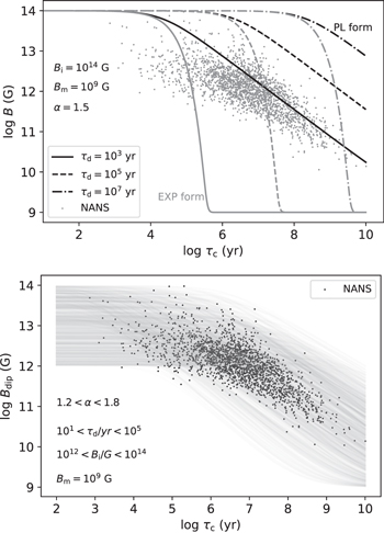
Figure 2. Surface dipole magnetic field strength Bdip vs. the characteristic age τc of the NANSs (dots). In the upper panel, the gray and black lines display the exponential and power-law forms of the NANS magnetic field evolution tracks with τd = 103 (solid lines), 105 (dashed lines), and 107 (dotted–dashed lines) yr. This shows that the power-law form with adjustable parameters can well fit the Bdip–τc trend of the NANSs. In the lower panel, the gray lines indicate the power-law form with different parameters, which are listed in the diagram.
Download figure:
Standard image High-resolution imageAlthough the favored form of magnetic field evolution has been found, we cannot ascertain the age of the NS, since it is hard to detect its growth ring in observations. But in theory, one can calculate its characteristic (or spin-down) age,  , which is the only age that can be easily derived for NSs. We assume that there is an unknown relation between the physical age τ and τc of NSs, and we can express it as τ = ξ
τc, where the parameter ξ indicates the relation. Then, we can get the initial magnetic fields,
11
, which is the only age that can be easily derived for NSs. We assume that there is an unknown relation between the physical age τ and τc of NSs, and we can express it as τ = ξ
τc, where the parameter ξ indicates the relation. Then, we can get the initial magnetic fields,
11
using the surface dipole magnetic field strength  , as well as the initial spin period,
3. Results
3.1. The Model without Magnetic Field Decay
We first consider the model without magnetic field decay and compare the results with the similar model from FK 2006 in Figure 3, where the initial spin period is

The gray histograms in the upper and lower panels indicate the surface dipole magnetic field Bdip and the observed spin period Pobs distribution of the NANSs, respectively. The black histogram profile and the gray line indicate the initial magnetic field Bi and spin period Pi distribution from our model and FK 2006, respectively. It shows that the distribution of Bi in our results is similar to that of FK 2006, both of which follow lognormal distribution, while we obtain a smaller mean value. However, Pi also pursues lognormal distribution in our model, which is  ,
,  for ξ = 1. It is much different from the normal distribution of FK 2006. When we take ξ < 1 (Zhang & Xie 2011), i.e., we think the actual age of the NS is smaller than its spin-down age, the mean value of the Pi distribution becomes larger (
 for ξ = 0.9 and
  for ξ = 0.5), while the standard deviation does not change. When we take ξ > 1, we cannot get any value of Pi.
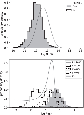
Figure 3. Distribution of the magnetic field (upper panel) and spin period (lower panel). The gray histograms and line indicate the magnetic field Bdip (the spin period Pobs) of the NANSs and the initial magnetic field Bi (the initial spin period Pi) distribution from FK 2006 in the upper (lower) panel, respectively. The black histograms in both panels show the Bi and Pi from our model, in which the solid, dashed, and dotted–dashed histograms in the lower panel represent the cases of ξ = 1, 0.9, and 0.5, respectively.
Download figure:
Standard image High-resolution image3.2. The Model with Magnetic Field Decay
Then we introduce magnetic field decay of NSs into the model, and it (top panel of Figure 2) shows that the power-law form (Equation (6)) is favored. We limit the parameters by fitting the distribution trend of NANSs in the Bdip–τc diagram (lower panel of Figure 2) in a rough range: 1.2 ≤ α ≤ 1.8 and 103 ≤ τd yr–1 ≤ 107. Then we try to simulate the initial values of the NANS magnetic field and spin period within the above parameter intervals.
Figure 4 displays the results of initial magnetic field distributions obtained by the control variable method. The variables are α, τd, and ξ from top to bottom, and other parameters are set to be α = 1.2, τd = 103 yr, and ξ = 1.0 when they are not variables. This shows that all Bi in our model can well fit the lognormal distributions with  and
and  . In the case with α = 1.2, τd = 103 yr, and ξ = 1.0, we get
  ,
,  , which is consistent with the last results in Igoshev et al. (2022).
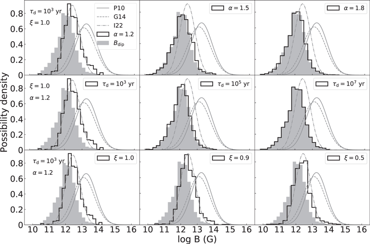
Figure 4. Initial magnetic field distributions with different parameters. The parameters are set as follows. Top panels: τd = 103 yr, ξ = 1.0, and α = 1.2, 1.5, and 1.8 from left to right. Middle panels: ξ = 1.0, α = 1.2, and τd = 103, 105, and 107 yr from left to right. Bottom panels: τd = 103 yr, α = 1.2, and ξ = 1.0, 0.9, and 0.5 from left to right. In comparison, the gray histograms display the distribution of the NANS Bdip, and the gray lines indicate the results from the literature, where the solid, dashed, and dotted–dashed lines are from Popov et al. (2010), Gullón et al. (2014), and Igoshev et al. (2022), respectively.
Download figure:
Standard image High-resolution imageWhen using the same parameters to simulate the spin periods, we can only get the initial values for some of the NANSs. Figure 5 shows the initial spin period distributions under the variables α, τd, and ξ from top to bottom, where the nonvariable parameters are set to be α = 1.2, τd = 105 yr, and ξ = 0.5. The percentage numbers in the figure labels indicate the proportion of the valid sample, which includes the NANSs for which we can get initial spin periods, to the total sample, which includes all of the NANSs. It shows that all of the Pi histograms favor lognormal distributions with  and
and  whether full or partial samples. The top row, the middle and middle right panels, and the bottom right panel share the same results as
  and
and  .
.

Figure 5. Initial spin period distributions with different parameters. The parameters are set as follows. Top panels: τd = 105 yr, ξ = 0.5, and α = 1.2, 1.5, and 1.8 from left to right. Middle panels: α = 1.2, ξ = 0.5, and τd = 103, 105, and 107 yr from left to right. Bottom panels: τd = 105 yr, α = 1.2, and ξ = 1.0, 0.9, and 0.5 from left to right. In contrast, the gray histograms display the distribution of the NANS Pobs, and the gray lines indicate the results from the literature, where the solid, dashed, and dotted–dashed lines are from Popov et al. (2010), Popov & Turolla (2012), and Igoshev et al. (2022), respectively. The percentage numbers in the labels indicate the proportion of valid samples to total samples, where the valid ones indicate the pulsars for which can get obtain Pi.
Download figure:
Standard image High-resolution image4. Discussion and Summary
In this work, we simulate the initial distribution of the magnetic fields Bi and spin periods Pi of NANSs, which are thought to have only undergone magnetic dipole radiation. Our result shows that both Bi and Pi favor lognormal distributions, while their values depend strongly on the parameters.
Since the relation ξ = τ/τc between the physical age τ and spin-down age τc of NSs is unknown, we take a linear one for simplicity. It shows that the mean value of Bi increases but that of Pi decreases as ξ becomes larger (lower panels of Figures 4 and 5). Furthermore, ξ has little effect on the mean value of Bi (lower panels of Figure 4) but a big effect on Pi (lower panels of Figures 3 and 5). In some situations, the simulation cannot give the Pi values for some sources (Figure 5). This is because the integration term in Equation (2) may be larger than the square term of the observed spin period, i.e., there may be  in some cases if the age in the integration is larger than the physical age of the pulsars. So we think the unknown relation should meet the condition ξ ≤ 1 (Zhang & Xie 2011). The upper panels of Figures 4 and 5 indicate that the mean value of Bi increases as the parameter α becomes smaller, while there is nearly no difference among the histogram lines of Pi. The effect of the parameter τd is opposite to that of ξ, i.e., the mean value of Bi decreases but that of Pi increases as τd becomes larger (middle panels in Figures 4 and 5).
The following arguments may lead to the initial distributions depending strongly on parameters in our simulation.
- 1.The NANSs we picked are probably not representative of the pulsars, which have only undergone magnetic dipole radiation. In fact, most of the pulsars may experience other processes of losing angular momentum, such as glitches (Espinoza et al. 2011), accretion (Ghosh & Lamb 1979), or magnetized stellar wind (Bisnovatyi-Kogan 2017).
- 2.
- 3.The relation between the physical and spin-down ages of NSs may be more complex than a linear one (Camilo et al. 1994).
However, since our sample is large enough and the physical age of the NSs is too hard to detect, our result is still somewhat informative.
We thank the anonymous referee for helpful comments and suggestions. This work was supported by the Natural Natural Science Foundation of China (NSFC, grant Nos. 11988101, 12203051, 11933004, 12041301, 12063001, 11773015), project funded by China Postdoctoral Science Foundation No. 2021M703168.
Footnotes
- 7
This is the value of the magnetic field at the equator, and the surface mean value is
 (Popov et al. 2010).
 - 8
- 9
As described above, it is very hard to select NANSs using the observed data, so we study the NANS candidate sample as a substitute.
- 10
- 11
In general, Bm is much smaller than Bi, so we ignore the terms including it here and in the equation of Pi.