


Abstract
In 2009, the Interstellar Boundary Explorer (IBEX) discovered a narrow "ribbon" of energetic neutral atom emissions across the sky with properties correlated with the solar wind latitudinal structure and the interstellar magnetic field draped around the heliosphere. It is widely believed that the ribbon is formed from the escape of heliospheric ENAs into the local interstellar medium and their eventual return as secondary ENAs. However, there is no consensus on the rate of pitch angle scattering of these PUIs before they become secondary ENAs. We test two opposing limits of scattering rates ("weak" versus "strong") by solving a time-dependent model of the ribbon that evolves with the solar cycle, and we compare them to IBEX observations over 2009–2019. First, we find that both models qualitatively reproduce the evolution of IBEX fluxes for most of the data set, with a few exceptions, although the strong (or "spatial retention") scattering model greatly underestimates the observed fluxes. Regardless, time dependence of fluxes cannot distinguish these models. Second, the ribbon's geometric properties, i.e., its center and radius, are significantly different between the models. The spatial retention model reproduces the observed ribbon centers as a function of energy and time slightly better than the weak scattering model, and the spatial retention model reproduces the observed ribbon radius over energy and time almost perfectly, whereas the weak scattering model compares poorly. Our analysis favors the spatial retention mechanism as the source of the IBEX ribbon, but it requires modification to increase the flux of ENAs observed at 1 au.
Export citation and abstract BibTeX RIS

Original content from this work may be used under the terms of the Creative Commons Attribution 4.0 licence. Any further distribution of this work must maintain attribution to the author(s) and the title of the work, journal citation and DOI.
1. Introduction
Since 2009, the Interstellar Boundary Explorer (IBEX; McComas et al. 2009a) has been observing the outer heliosphere via measurements of energetic neutral atom (ENA) emissions. Equipped with two single-pixel cameras, IBEX observes full-sky ENA emissions from ∼0.1 to 6 keV every six months. While it was predicted that IBEX would observe "globally distributed fluxes" with smooth, spatially varying enhancements from the nose and tail directions of the heliosphere (Heerikhuisen et al. 2008; Prested et al. 2008; McComas et al. 2009a), IBEX discovered a circular band of enhanced ENA emissions dubbed the "ribbon" (McComas et al. 2009b). This unexpected observation led to numerous theories for its origin (McComas et al. 2014), one of which is the secondary ENA mechanism. It was quickly shown that the ribbon was correlated with the interstellar magnetic field (ISMF) draped around the heliosphere (Schwadron et al. 2009), and models based on the secondary ENA mechanism were generally able to reproduce the observations (Chalov et al. 2010; Heerikhuisen et al. 2010; Schwadron & McComas 2013; Zirnstein et al. 2013).
Currently, it is widely accepted that the ribbon is formed by the secondary ENA mechanism. ENAs created in the outward-propagating solar wind (SW) or from the inner heliosheath (IHS) exit the heliosphere into the denser local interstellar medium (LISM). These ENAs eventually charge exchange with interstellar ions, producing pickup ions (PUIs) that gyrate around the ISMF lines. The PUIs will neutralize again after a period of time depending on the PUI energy and the local neutral density, and they may travel back into the heliosphere. Due to their long mean free paths inside the heliosphere, some of these "secondary" ENAs can travel close to the Sun and be observed by IBEX. The ribbon, therefore, is likely formed from secondary ENAs whose intensity is greatest where the observer's line of sight ( r ) is approximately perpendicular to the ISMF ( B ) draped around the heliosphere, i.e., B · r = 0. The B · r = 0 plane is warped as a function of distance from the heliopause by the draping of the ISMF around the heliosphere (Pogorelov et al. 2011), forming a complex, 3D structure of the ribbon source region as a function of ENA energy (Zirnstein et al. 2015).
It has been shown that the ribbon's intensity and overall structure depends on the pitch angle scattering behavior of PUIs as they gyrate around the ISMF before becoming secondary ENAs (Schwadron et al. 2018; Zirnstein et al. 2019a, 2021a). It also depends on the local interstellar turbulence power spectrum (Burlaga et al. 2018) and how efficiently PUIs are pitch angle scattered or are able to maintain anisotropy near B · r = 0 (also referred to as the "spatial retention region"; see Liu et al. 2012; Schwadron & McComas 2013; Isenberg 2014; Summerlin et al. 2014; Florinski et al. 2016; Gamayunov et al. 2017; Giacalone & Jokipii 2020; Zirnstein et al. 2020a; Mousavi et al. 2022a, 2022b, 2022c). It is still not clear how PUIs behave over the course of their lifetime as ions (e.g., the 1/e charge exchange lifetime for a 1 keV H+ PUI within a surrounding neutral H gas with density 0.2 cm−3 is ∼2.1 yr, and for a 4 keV H+ PUI it is ∼1.6 yr) and the net effect it has on the observed ribbon structure. However, it is clear that PUIs undergo some level of scattering due to their initially unstable ring beam distributions, but they cannot become completely isotropic in velocity space—otherwise the ENA intensity observed at 1 au will be too small (Heerikhuisen et al. 2014; Isenberg 2014; Zirnstein et al. 2019a).
Although it is not fully understood how PUIs behave in the secondary ENA process, the evolution of the IBEX ribbon clearly changes with the solar cycle, delayed by a few years compared to changes in the GDF (McComas et al. 2017, 2020; Schwadron et al. 2018; Swaczyna et al. 2022). In this study, we propose that the evolution of the IBEX ribbon over solar cycle 23 may help us differentiate the role of PUI pitch angle scattering, either due to differences in the evolving ribbon intensity or its geometric structure, i.e., ribbon center and radius (Dayeh et al. 2019). We test this hypothesis by solving our weak scattering (Zirnstein et al. 2018) and strong scattering (Zirnstein et al. 2019a) ribbon models with time-dependent neutral SW and interstellar PUI sources, as described in Section 2. In Section 3, we compare our ribbon model results (evolution of intensity, center, and radius) as a function of ENA energy with IBEX ribbon data separated from the GDF using spherical harmonic decomposition (Swaczyna et al. 2022).
2. Model Description
2.1. Global Simulation of the Heliosphere
As with our previous studies on modeling the IBEX ribbon (Zirnstein et al. 2013, 2015, 2018, 2019a, 2019b, 2020a, 2021a), we utilize results from a three-dimensional, global magnetohydrodynamic (MHD) simulation of the SW-LISM interaction based on MS-FLUKSS (Pogorelov et al. 2008; Heerikhuisen et al. 2015), where we simulate secondary ENA fluxes from outside the heliopause using different assumptions for PUI pitch angle scattering: weak pitch angle scattering (Zirnstein et al. 2018) or strong pitch angle scattering using the spatial retention model (Schwadron & McComas 2013; Zirnstein et al. 2019a). The heliosphere simulation solves ideal MHD equations for a single-fluid plasma and the Boltzmann equation for propagation of neutral H atoms. The plasma and neutrals are coupled by charge-exchange source terms (Heerikhuisen et al. 2015).
The SW boundary conditions at 1 au for the steady-state heliosphere simulation are chosen to be the same as those used by Zirnstein et al. (2021b). At low latitudes (<∣ ±37°∣, from the OMNI database in 2004–2009), the SW speed is 449 km s−1, plasma density is 6.53 cm−3, temperature is 1.02 × 10⁵ K, and radial magnetic field component is 37.4 μG. At high latitudes (>∣ ±37°∣, from Ulysses' third polar scan (McComas et al. 2008)), SW speed is 743 km s−1, density is 2.23 cm−3, temperature is 2.98 × 10⁵ K, and radial magnetic field component is 34.7 μG.
The LISM boundary conditions are applied at 2500 au from the Sun, which we note is larger than the 1000 au outer boundary we have used in previous studies. The radial grid resolution in the ribbon source region ranges from Δr = 0.9 to 1.3 au for r = 120–200 au. The angular resolution is (Δθ, Δφ) = (1 5, 20), which is sufficiently small to capture the structure of the modeled ribbon (whose width is >10°). The LISM boundary conditions are chosen based on IBEX, Voyager, and New Horizons (NH) SWAP observations. The pristine magnetic field vector is pointed toward (22728, 3462) in ecliptic J2000 with magnitude 2.93 μG (Zirnstein et al. 2016b). The interstellar plasma number density is 0.09 cm−3, and the neutral H number density is 0.17 cm−3. Our steady-state model overestimates the thickness of the heliosheath, such that we cannot simultaneously reproduce both the heliospheric termination shock (HTS) and heliopause distances observed by the Voyagers. Therefore, this combination of LISM number densities is designed such that the middle of the simulated heliosheath, averaged in the Voyager 1 and 2 directions, approximately agrees with the average of Voyager 1 and 2's observations of the middle of the heliosheath. Finally, similarly to Zirnstein et al. (2021b), we assume that 4% of the plasma density in the SW consists of alpha particles and 10% of the plasma density in the LISM consists of He+ ions, such that those percentages of the ions are not included in the H–H+ charge-exchange source terms of the MHD-kinetic model of the heliosphere. This ad hoc modification of the plasma density in the charge exchange source terms yields a filtrated interstellar neutral H density at the upwind HTS of ∼0.13 cm−3, in agreement with extrapolations from NH SWAP observations (Swaczyna et al. 2020).
2.2. Outward-propagating Neutral Source Terms
The neutral particles that are the parent population for PUIs outside the heliopause originate from (1) protons in the supersonic SW, i.e., the core SW protons, (2) interstellar H+ PUIs embedded in the outward-propagating SW, and (3) hot ions in the IHS that were accelerated at the HTS. The neutralized SW source of the ribbon has been included in all past secondary ENA models (Chalov et al. 2010; Heerikhuisen et al. 2010; Schwadron & McComas 2013; Zirnstein et al. 2013). Neutralized hot heliosheath ions have been included in several studies of the "partial shell" model of the ribbon using kinetically driven neutral source terms (Heerikhuisen et al. 2010; Zirnstein et al. 2013, 2016a), but these studies suggest heliosheath neutrals do not contribute significantly to the ENA fluxes measured by IBEX-Hi below ∼6 keV, and therefore we do not include them. The inclusion of neutralized interstellar H+ PUIs in our current study, however, is motivated by the analysis of Schwadron & McComas (2019), who showed that these particles may produce the majority of ENAs in the IBEX-Hi ESA 4–6 passbands (∼2–6 keV). As we will show in our study, the neutralized core SW component (hereafter called NSW) generally dominates the ribbon signal at energies ≲2 keV, and the neutralized interstellar H+ PUIs in the SW (hereafter called NPI) dominates the source of the ribbon signal at energies >2 keV. The latitudinal distribution of their contributions to the ribbon are also distinctly different, due to their vastly different thermal energies in the SW frame.
One main difference in this study compared to our previous work is that we calculate NSW and NPI fluxes for individual years (time t) based on the IPS-based empirical model of Sokół et al. (2020). Because IPS-based SW speeds generally overestimate near-ecliptic in situ measurements (Tokumaru et al. 2021), the SW speed is subtracted by a constant value uniformly at all latitudes to match OMNI at low latitudes. However, it is unclear whether IPS-derived speeds should be shifted uniformly in speed at all latitudes, or differently in the northern and southern hemispheres, or not at all except near the ecliptic plane. Therefore, we also present results where no shifting is performed in order to understand the effects of this assumption on our ribbon model results. The SW density is determined by taking measurements from the OMNI database over a similar time period, namely the central time from the IPS model ±0.375 yr and calculating the density as a function of latitude, assuming the dynamic pressure is constant with latitude. We also assume the SW temperature is constant over latitude and time (see Section 2.2.1, Equation (4)). While this is not strictly true, the effects of SW temperature on the model results are small compared to the radial spread of the distribution. The PUI temperature is modeled more accurately using the filled-shell distribution as a function of distance from the Sun (see also Sections 2.2.2 and 2.2.3).
2.2.1. Neutral SW H+ Flux
Building upon our previous work (Swaczyna et al. 2016; Zirnstein et al. 2019a, 2019b), we model the NSW source term by integrating the flux of neutralized SW H+ from 1 au to the HTS for SW conditions derived from IPS observations by Sokół et al. (2020). We calculate the NSW flux for each annual time period, denoted by time tj , where j is the index corresponding to years shown in Table A1 of Sokół et al. (2020):

where NMB is the Maxwell–Boltzmann speed distribution, uSW is the SW speed slowing with distance from the Sun, and λml is the mean free path length for neutralization of SW protons. The term  in the exponential function is the arithmetic mean of neutral H density from r0 to r in direction
  . Because the rates of photoionization for H and He are small compared to H–H+ charge exchange, we assume they are constant in time with values at r0 = 1 au of νH = 1.3 × 10⁻⁷ s−1 and νHe = 1 × 10⁻⁷ s−1 (Sokół et al. 2020). We integrate the SW flux (first term), as it adiabatically expands to the HTS and attenuates due to charge exchange losses (exponential term), multiplied by the probability of charge exchange with neutral H, and multiplied by a one-dimensional Maxwell–Boltzmann speed distribution to account for variations in SW speed that occur over approximately ∼1 yr intervals (i.e., the cadence of the IPS-derived SW speed model). To do this, first we find the standard deviation of SW speed at 1 au from the OMNI database corresponding to the IPS measurement times (which is typically δ
vu
∼ 100 km s−1 at 1 au) and use New Horizons SWAP observations of SW speeds between 20 and 40 au from the Sun to determine how the speed deviation δ
vu
changes with distance. We find from SWAP observations that the SW speed spread drops significantly at large distances (becoming δ
vu
∼ 25 km s−1 halfway to the HTS). We find a best-fit power-law relation between OMNI and SWAP observations of the SW speed standard deviation (testing bin sizes between 0.5 and 2 yr, which asymptotically yields a power-law slope of −0.37 for 2 yr bins), such that
. Because the rates of photoionization for H and He are small compared to H–H+ charge exchange, we assume they are constant in time with values at r0 = 1 au of νH = 1.3 × 10⁻⁷ s−1 and νHe = 1 × 10⁻⁷ s−1 (Sokół et al. 2020). We integrate the SW flux (first term), as it adiabatically expands to the HTS and attenuates due to charge exchange losses (exponential term), multiplied by the probability of charge exchange with neutral H, and multiplied by a one-dimensional Maxwell–Boltzmann speed distribution to account for variations in SW speed that occur over approximately ∼1 yr intervals (i.e., the cadence of the IPS-derived SW speed model). To do this, first we find the standard deviation of SW speed at 1 au from the OMNI database corresponding to the IPS measurement times (which is typically δ
vu
∼ 100 km s−1 at 1 au) and use New Horizons SWAP observations of SW speeds between 20 and 40 au from the Sun to determine how the speed deviation δ
vu
changes with distance. We find from SWAP observations that the SW speed spread drops significantly at large distances (becoming δ
vu
∼ 25 km s−1 halfway to the HTS). We find a best-fit power-law relation between OMNI and SWAP observations of the SW speed standard deviation (testing bin sizes between 0.5 and 2 yr, which asymptotically yields a power-law slope of −0.37 for 2 yr bins), such that
Because we do not know the variation of SW speeds at high latitudes except from Ulysses observations before 2009, we make a simplified assumption that the SW speed standard deviation scales linearly with SW speed. This is motivated by the fact that, as the Sun rotates over time, the mid-latitude SW streams create stream interactions and thus larger speed variations. This assumption does break down at high latitudes during solar minimum when the SW speed appears steady (McComas et al. 2008), likely affecting the northern section of the ribbon model above +40° latitude, i.e., the ribbon "knot."
We also include a term for the thermal motion of the SW,


where we have assumed a constant SW proton temperature of 9 × 10⁴ K at 1 au, for simplicity. The exponent in Equation (3) is also derived by fitting a power-law relation between OMNI and 1 yr binned SWAP observations of SW proton temperature. This yields the total speed deviation,

We note that the second term in Equation (5) is small compared to the first term and can be neglected.
The NSW flux decreases with distance beyond the HTS due to adiabatic expansion and due to losses by charge exchange outside the heliopause (where plasma densities are much higher than inside the heliopause), yielding (Zirnstein et al. 2021a)

2.2.2. Neutral Interstellar PUI H+ Flux
In contrast to SW protons, which can be approximately described with a Maxwell–Boltzmann speed distribution, interstellar PUIs are characterized by a nonthermalized, filled-shell distribution, due to the process in which they are injected into the SW and scatter in pitch angle (Vasyliunas & Siscoe 1976), in addition to experiencing nonadiabatic cooling with distance from the Sun (McComas et al. 2021). The NPI flux source term is therefore given as

The function NFS is based on the generalized filled-shell distribution (Chen et al. 2013; Swaczyna et al. 2020; McComas et al. 2021) integrated over the speed components perpendicular to the radial direction. The PUI cooling index is α ≅ 2.1 halfway to the HTS (McComas et al. 2021), therefore we assume α = 2.1 is constant with distance r in Equation (7). β is the angle between the SW radial vector and the LISM H inflow vector assumed to be moving at uH = 22 km s−1 (Lallement et al. 2010). The neutral H density term in Equation (7) is evaluated at distance rwα
, to compensate for the ionization cavity effect for neutral H close to the Sun. The interstellar PUI density  is calculated from first-order solutions to fluid transport equations from, e.g., Lee et al. (2009):

Similarly to the NSW flux (Section 2.2.1, Equation (6)), the NPI flux decreases in intensity beyond the HTS, due to adiabatic expansion and charge-exchange losses.
Examples of the NSW and NPI flux at the upwind HTS are shown in Figure 1. In general, the NSW flux has a narrower, more intense distribution centered near the SW speed at a given latitude (blue curves). The NPI fluxes are lower in intensity near the bulk SW speed but are more thermally broad, extending to lower and higher energies. The NPI flux does not have a sharp cutoff like the PUI distribution (McComas et al. 2021), because the radially integrated NPI flux includes PUIs created at different distances from the Sun, which were scattered onto shells with different cutoff speeds, due to the slowing of the SW with distance from the Sun. The NPI flux also has a minimum at the bulk SW speed (e.g., 0.3 keV in Figure 1(a)), corresponding to PUIs with very low speeds in the SW frame—which, however, could not be created, due to significant losses of neutral H inside the ionization cavity close to the Sun (Sokół et al. 2019).

Figure 1. NSW and NPI flux at the upwind HTS as a function of energy. (a)–(c) Fluxes produced from IPS observations made in 2009. (d)–(f) Fluxes produced from IPS observations made in 2014. We show fluxes at heliolatitudes of (a), (d) 0°, (b), (e) 30°, and (c), (f) 60°.
Download figure:
Standard image High-resolution imageWe show examples of NSW and NPI fluxes in 2009 and 2014, which reflect solar minimum and maximum conditions, respectively, in solar cycle 24. At low latitudes (Figures 1(a) and (d)), the neutral fluxes are similar at both times in the cycle. At 30° latitude, which is approximately the latitude at which the polar coronal holes (PCH) reach their lowest point during solar minimum, the NSW and NPI fluxes shift to higher energies in 2009. At 60° latitude, well within the northern PCH and at a latitude similar to the ribbon knot seen at 2.73 keV, the NSW and NPI fluxes reach their highest energies in 2009, due to fast SW from the PCH. Moreover, the NSW distribution is more flat-topped, which appears to be a result of a larger spread of SW speeds as defined in Equation (2), which increases with higher SW speeds. As we stated earlier, it is not clear if this assumption is correct at high latitudes, but we believe it is reasonable at latitudes <∣ ± 60°∣ near solar minimum and all latitudes near solar maximum.
We note that, in this study, we only consider neutral sources inside the HTS, which have been shown to be an essential component of the ribbon source. However, neutralized PUIs from the IHS will also contribute to the ribbon source signal, although we expect this to occur at low intensities from ∼0.5 to 3 keV. Above ∼3 keV, hot heliosheath neutrals may be a significant source for the ribbon signal (Zirnstein et al. 2016a; Schwadron & McComas 2019). This component will be analyzed and included in a future study.
2.2.3. Neutral SW and PUI Source Transverse Components
As we discuss the NSW and NPI distributions beyond the HTS, first it is important to note that, from hereafter, we refer to the local time variable as t, such that  , which is the time in the past when the ENA traveling at speed v was created at LOS length distance l from IBEX.
In this study, we model the ribbon in the limits of weak pitch angle scattering (Zirnstein et al. 2018) and strong pitch angle scattering (Schwadron & McComas 2013; Zirnstein et al. 2019a). In the limit of weak pitch angle scattering, we assume the NSW and NPI distributions outside the heliopause have thermal spreads transverse to the radial direction, with different temperatures. The transverse component of Equations (1) and (7) are given as (Zirnstein et al. 2021a)


where H is the Heaviside step function, and  is the PUI velocity vector with the same magnitude as the ENA
  with pitch angle φ and gyro-phase ω. The transverse temperature at the HTS, T⊥,i,HTS, for neutral component i (NSW or NPI) is


For simplicity, we assume the NSW temperature at the HTS is constant, a justifiable assumption due its small thermal spread (Florinski & Heerikhuisen 2017) compared to the width of the IBEX ribbon. The NPI temperature is much larger, however, and therefore we approximate its temperature using a weighted average of the interstellar PUI temperature from r0 to rHTS, weighted by the local PUI and neutral H densities. The interstellar PUIs, once neutralized, will have a temperature that decreases due to adiabatic expansion, hence the r2 term in the first part of Equation (11). The interstellar PUI temperature T⊥,PI is taken from Zirnstein et al. (2022). The weighting term WNPI accounts for the number density of PUIs that, once neutralized by charge exchange with the local neutral H density, will also adiabatically expand with distance to the HTS.
The NPI distribution is much hotter than the NSW, and because of our approach to modeling the ribbon, our methodology does not account for the fact that we might produce PUIs whose initial pitch angle vectors do not originate from within the HTS. Therefore, we add one final criterion to the NPI source, by excluding any PUI whose initial velocity vector angle from the radial direction is larger than  , where 90 au roughly approximates the average HTS distance in the nose-ward hemisphere (where most of the ribbon appears in the sky). We note, however, that this exclusion yields a negligible change in our results.
2.3. Time-dependent ENA Flux Calculation
The time-dependent, differential ENA flux at 1 au is calculated as

where  is the PUI distribution function along the IBEX line of sight (LOS) vector direction (θ, ϕ) for the weak or strong scattering models of the ribbon, following the work of Zirnstein et al. (2021a) (see their Equations (4), (6), and (9)), and
  is the probability of ENA survival from their point of creation to the HTS (it should be noted that we compare to IBEX data corrected for ENA losses from 100 au, i.e., near the HTS, to 1 au). The integration is performed along the IBEX LOS from the heliopause (rHP) to the outer boundary set at 700 au from the Sun (rOB). As stated in Section 2.2.3, the time variable is t = t0 − l/v, where l is the distance traveled by the ENA with speed v backward in time along the IBEX LOS. The variable t0 is chosen as a function of longitude and latitude to coincide with IBEX's measurement times as it takes observations over the course of a full year in the "ram" frame.
2.3.1. Weak Scattering Model ENA Source
Because this study simulates time-dependent ENA flux, for completeness, we rewrite the equations for f0 from Zirnstein et al. (2021a). The time-dependent PUI distribution in the weak scattering model is the same for both the NSW and NPI sources:

where  is the 1/e charge-exchange timescale for neutralizing protons at relative interaction speed vrel. The neutral source function is
Similarly to our previous work (Zirnstein et al. 2020b), we assume the initial PUI ring beam scatters onto a narrow partial shell with width Δφ = 5° centered on the initial pitch angle φ, and we integrate over gyro-phase ω assuming a uniform distribution over the partial shell. Our assumption of Δφ = 5°, as we tested in Zirnstein et al. (2020b), does not significantly affect our ribbon intensities compared to assuming 2° or 10°. We expect even less effect on the ribbon geometry because of the symmetry of Δφ around the initial pitch angle. The position vector  signifies the position of the PUI traced backward in time, using guiding center motion, created at time
  , where tg
is the elapsed time for the guiding center motion of the PUI. The main difference in Equation (13) compared to Zirnstein et al. (2021a) is that the integration backward in time solves for a time-dependent source for the NSW or NPI flux, Si
, rather than assuming it is constant over time. The total PUI distribution is given as
, where tg
is the elapsed time for the guiding center motion of the PUI. The main difference in Equation (13) compared to Zirnstein et al. (2021a) is that the integration backward in time solves for a time-dependent source for the NSW or NPI flux, Si
, rather than assuming it is constant over time. The total PUI distribution is given as  .
.
2.3.2. Strong Scattering Model ENA Source
We simulate the ribbon in the strong scattering limit using the spatial retention mechanism (Schwadron & McComas 2013), separately for the NSW and NPI sources. For the case where PUIs are created from the NSW, where the effects of the small thermal spread of the NSW can be neglected (Schwadron & McComas 2013), the time-dependent PUI distribution inside the retention region is
and outside the retention region it is
where  is the distance along the local ISMF line,
 ![${\tau }_{1}=1/\left[2/{\tau }_{\mathrm{sc}}+1/{\tau }_{\mathrm{ex}}\right]$](https://content.cld.iop.org/journals/0004-637X/949/2/45/revision1/apjacc577ieqn15.gif) , and τsc = λ∥/v is the PUI pitch angle scattering timescale with mean free path λ∥. The NSW source function is
, and τsc = λ∥/v is the PUI pitch angle scattering timescale with mean free path λ∥. The NSW source function is

More details on the derivation of Equations (15) and (16), specifically  and τ1 (which is the effective timescale for either charge exchange or pitch angle scattering to occur), can be found in Schwadron & McComas (2013) and their application in our global MHD simulations in Zirnstein et al. (2019a, 2021a).
In our past work, we assumed that the rate of PUI pitch angle scattering, 1/τsc, outside the retention region was either much faster than charge exchange or much slower than charge exchange, with the former yielding a broad background of ENA flux, like the GDF, in directions far from the ribbon (see Figures 6 and 7, second rows, in Zirnstein et al. (2019a)). The intent of the current study is to compare our simulation results to the separated ribbon data from Swaczyna et al. (2022), who separated out the GDF, which may have a component originating from outside the heliopause. Therefore, we present simulation results for the case of slow pitch angle scattering outside the retention region, which does not produce a GDF-like signature outside the ribbon region. In this limit where τex << τsc, Equation (16) approaches zero. We do not expect that our main results would change significantly if we simulated fast pitch angle scattering outside the retention region and then post-processed the modeled ribbon by removing the "background" similarly to the GDF removal by Swaczyna et al. (2022). This is because the key characteristics of the retention model are the enhancement in PUI density in the middle of the retention region and the closer proximity of the ribbon source to the heliopause than in the weak scattering case.
For the case where PUIs are created from the NPI distribution, which is much hotter than the NSW distribution, we must integrate over the NPI distribution similarly to the weak scattering case. Thus, inside the retention region,

where we integrate over solid angle Ω in phase space. It should be noted, again, that we exclude any creation of PUIs whose initial velocity vectors would not originate within the HTS (see the end of Section 2.2.3). The NPI source function  is the same as Equation (14), except we combined Ω = (ω, φ) for simplicity.
3. Results and Discussion
In this section, we compare our modeling results to IBEX observations of the ribbon separated from the GDF using spherical harmonic decomposition by Swaczyna et al. (2022). First, we calculate the solar cycle averaged maps for IBEX data and our two ribbon models at each ESA, shown in Figure 2. It should be noted that the color bar range is the same for both models and the data, except that spatial retention model results are scaled up by a factor of 4 for comparison to the data. This required scaling is a continuing issue of the spatial retention model when implemented in our global MHD simulation (Zirnstein et al. 2019a, 2021a), which we discuss further in Section 4.
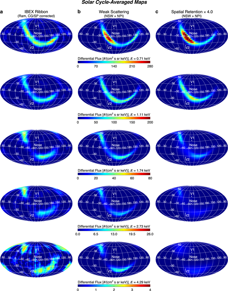
Figure 2. Solar cycle averaged maps of the IBEX ribbon data and modeling results. (a) Sky maps of IBEX ribbon data, derived from the ribbon separation technique in Swaczyna et al. (2022). (b) Sky maps of modeled ribbon assuming weak pitch angle scattering. (c) Sky maps of modeled ribbon assuming strong pitch angle scattering in the spatial retention mechanism.
Download figure:
Standard image High-resolution image3.1. Solar Cycle Averaged Sky Maps
The solar cycle averaged maps in Figure 2 showing reasonable similarity between the data and weak scattering model, in both intensity and structure. However, both models clearly underestimate the flux from the ribbon knot (high northern latitudes at energies >1 keV), likely due to our assumption for the SW speed variability as discussed in Section 2.2.1 and Equation (2). Both models also show relatively high intensity close to the ecliptic plane at energy ∼0.7 keV compared to mid latitudes, while the data show a more uniform distribution of flux at all latitudes at this energy. The reason for this discrepancy is unclear, but is likely related to either (1) inaccuracies in the ribbon separation and/or (2) inaccuracies in the SW speed model derived from IPS observations. First, the IBEX maps at ∼0.7 keV that include both the GDF and ribbon flux also show the highest intensities along the ribbon near the ecliptic plane, but this effect may have been removed in the ribbon-separated maps due to a localized GDF maximum near the nose coinciding with this portion of the ribbon. Second, while we shift IPS-derived SW speeds near the ecliptic plane to match OMNI, this shift is performed uniformly at all latitudes. If we trust the accuracy of the OMNI database of observations, then it is possible the model ribbon fluxes at mid-to-high latitudes are underestimated at energies near ∼0.7 keV (or SW speeds near ∼350 km s−1). Either way, this is an example of the issues with understanding high-latitude SW speeds from IPS without in situ measurements.
3.2. Sky Maps of the Ribbon over a Solar Cycle
Next, we show the results of our time-dependent ribbon models from 2009 to 2019. The results are calculated in the same frame of the spacecraft (specifically the "ram" frame) and the same measurement time per longitudinal swath as Earth, and thus IBEX, orbited the Sun each year (McComas et al. 2010). The model results are also integrated over the IBEX ESA response functions (Funsten et al. 2009). Figure 3 shows results for the ribbon at ESA 3 (∼0.8–1.6 keV) for annual ram maps from 2009 to 2019. In general, the agreement between the models and data are good, where there is a gradual decrease in ENA intensity from ∼2011 to 2016, after which the fluxes level out. Then, in 2019, the southern portion of the ribbon appears to brighten in both the data and model results. This is likely a direct response to changes in the SW dynamic pressure (both speed and density) in the middle of solar cycle 24 (McComas et al. 2020). There is not much structural difference between the two models, at least at 6° pixel resolution (Zirnstein et al. 2019a, 2019b), besides the significant difference in total intensity.
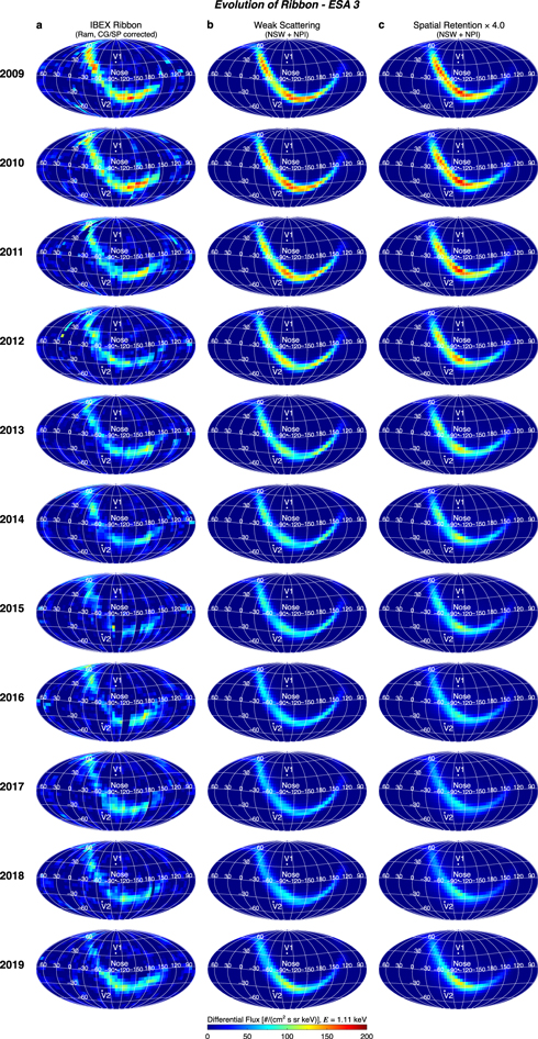
Figure 3. Sky maps of IBEX ribbon data and modeling results at ESA 3 from 2009 to 2019. (a) Sky maps of IBEX ribbon data. (b) Sky maps of modeled ribbon assuming weak pitch angle scattering. (c) Sky maps of modeled ribbon assuming strong pitch angle scattering in the spatial retention mechanism.
Download figure:
Standard image High-resolution imageFigure 4 shows results for the ribbon at ESA 5 (∼2.0–3.8 keV). Again, there is general agreement between the data and model results, although the difference in intensity between the spatial retention model and the data is even more pronounced. This implies that the discrepancy between the data and spatial retention model intensities is energy dependent. Notwithstanding this issue, there is clearly a decrease in ribbon intensity from ∼2012 to 2016, and a hint of brightening occurring in the weak scattering model south of the ecliptic plane but not visibly in the spatial retention model.

Figure 4. Similar to Figure 2, except for fluxes measured in ESA 5.
Download figure:
Standard image High-resolution image3.3. Contribution of NSW versus NPI to the Ribbon
We have not yet discussed how the NSW and NPI sources contribute to the overall intensity and structure of the ribbon in the models. Due to their significantly different distributions in energy (Figure 1), we should expect that they have energy-dependent effects on the ribbon. In Figure 5, we show sky maps of the weak scattering ribbon model in 2009 for each ESA, where we separate the components of the ribbon from the NSW (left column) and NPI (middle column), alongside the total (right column). From Figure 5, one can see that the NSW dominates the source of the ribbon signal at ESA 2 and 3, because the NSW flux has the highest intensity near the SW speed which, at low-to-mid latitudes, is near the ENA energies measurable by ESA 2 and 3 (∼0.5–1.6 keV). At ESA 4, we see an increased contribution from the NPI to the ribbon source almost uniformly at all latitudes, due to its large thermal spread. At ESA 5, the NSW only appears to contribute to the knot at high northern latitudes, while the NPI dominates the rest of the ribbon structure. At ESA 6, the NPI source completely dominates the ribbon signal in the sky. The highest SW speeds are typically ∼750 km s−1, which lies in the middle of ESA 5. Therefore, the hotter NPI fluxes are the dominant source of the ENA signal observed in ESA 6.
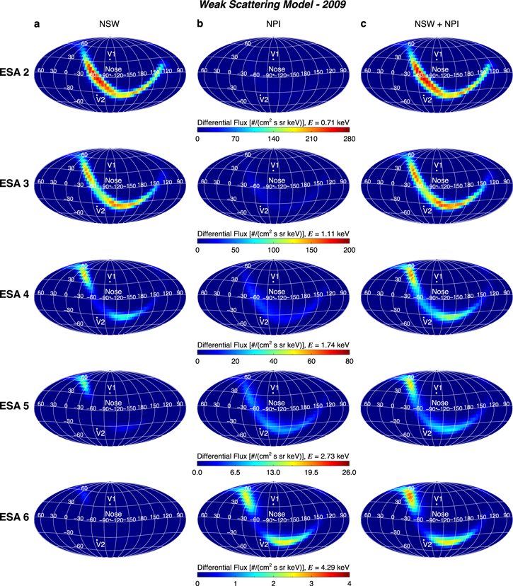
Figure 5. Sky maps of the weak scattering ribbon model at ESA 2–6 for 2009. (a) Ribbon fluxes produced from neutral SW (NSW). (b) Ribbon fluxes produced from neutral PUI (NPI). (c) Total ribbon fluxes.
Download figure:
Standard image High-resolution imageFigure 6 shows results similar to those in Figure 5, except for the spatial retention model of the ribbon. While the relative contribution of the NSW versus NPI to the source of the ribbon is similar to that in the weak scattering model, the NPI component is more broadly spread out in the sky and does not exhibit a narrow ribbon-like structure. This behavior may be consistent with part of the GDF or the wider ribbon observed at higher energies (Fuselier et al. 2009; Schwadron et al. 2011). Similarly to the weak scattering model, here the NSW dominates the ribbon knot seen in ESA 5, and the NPI component dominates the entire ribbon signal at ESA 6.
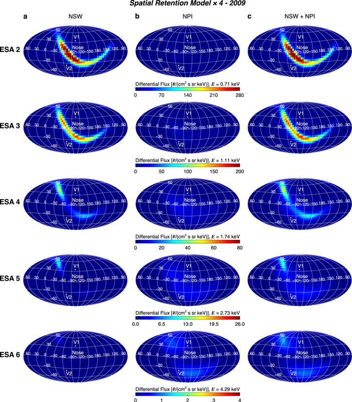
Figure 6. Similar to Figure 5, except for the spatial retention model. We note that the spatial retention model fluxes here are scaled by a factor of 4.
Download figure:
Standard image High-resolution imageThe energy dependence of the ribbon flux with the inclusion of NPI is illustrated in more detail in Figure 7. We extracted the model ribbon fluxes from a pixel near ecliptic longitude 256° and latitude −23°, i.e., about 28° below the nose of the heliosphere. The models without NPI, shown in blue, exhibit steep drop-offs in intensity at energies above 1 keV. With the inclusion of the NPI source, the ribbon spectra flatten in the IBEX-Hi energy range, yielding a power-law slope in energy of ∼E−3. This illustrates the importance of the NPI component for the source of the IBEX ribbon at energies >2 keV, for any secondary ENA ribbon source mechanism.
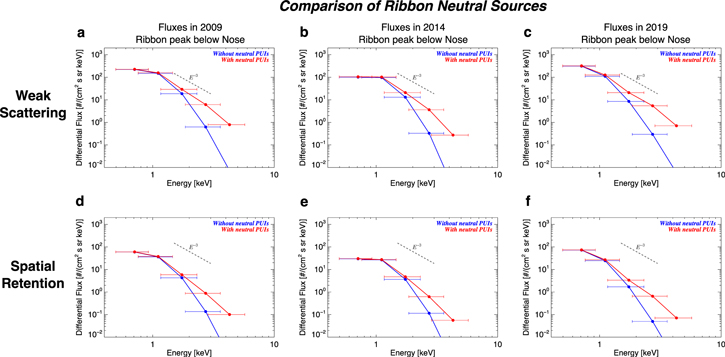
Figure 7. Comparison of ribbon ENA spectra with (red curves) and without (blue curves) the neutral PUI source, simulated in (a), (d) 2009, (b), (e) 2014, and (c), (f) 2019. Modeling results for the (a)–(c) weak scattering and (d)–(f) spatial retention mechanisms are shown. A power-law spectrum of E−3 is shown that approximately represents the average slope of the ribbon spectra when a source of neutral PUIs is included. The FWHM of the IBEX ESA energy steps are also shown as horizontal uncertainty ranges in energy.
Download figure:
Standard image High-resolution image3.4. Ribbon Time Series
In this section, we show the time series of the observed and modeled IBEX ribbon signal averaged over three regions of the sky. The three regions, as illustrated in Figure 8, are: (1) the "knot", where the highest intensity of the ribbon is observed at ESA 5 and 6; (2) the "ecliptic", which is centered around the ecliptic plane (which is also close to the solar equatorial plane, i.e., an angular difference of ∼1 IBEX pixel); and (3) the "south", which is the southern region of the ribbon. Each of these regions has a width (i.e., angular size perpendicular to the ribbon's circle) of ∼20°. Time series of the observed and modeled ribbon fluxes averaged over these three regions in the sky are shown in in Figure 9.

Figure 8. Sky map showing regions of the ribbon where fluxes are averaged for time series comparisons shown in Figure 9.
Download figure:
Standard image High-resolution image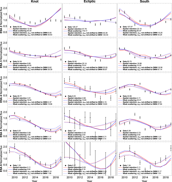
Figure 9. Time series of ribbon ENA fluxes from IBEX observations (black), the weak scattering model (blue), and the strong scattering model (red). We show modeling results where the IPS-derived SW speeds are scaled uniformly in latitude to match near-ecliptic OMNI data (solid curves) and where no scaling is performed (dashed curves). Each curve is individually normalized to the 11 yr average. The time-averaged value for each curve is shown in the labels in each panel.
Download figure:
Standard image High-resolution imageThe left, middle, and right columns show time series of ribbon fluxes from the knot, ecliptic, and south regions of the sky, respectively. We normalize the fluxes such that each time series (per ESA and region) has the same average over time. The factors used to scale the data and model results are shown next to the labels of the respective time series curves. We will discuss the significance of these scaling factors near the end of this section. We show modeling results where we shift the IPS-derived SW speeds by a value to match OMNI near the ecliptic plane, and this shift is performed uniformly at all latitudes. We also show results where no shift is performed.
In general, there is good agreement between the models and the data in terms of overall evolution with the solar cycle. First focusing on the ecliptic region results, in general there is a decline in ENA fluxes over all energies, with the start of a recovery beginning after 2018, depending on the ENA energy. Comparisons with data become difficult at ESA 5 and 6 in the ecliptic region, because there is little ribbon flux at low latitudes and data uncertainties of the separated ribbon are large. The models predict the greatest relative changes occur at the highest ESA, illustrating the energy-dependent influence of the SW as it changes over the solar cycle. It is important to note that there are stark contrasts in the models with and without modifying IPS-derived speeds to match OMNI. Clearly, if there is a difference between IPS speeds and in situ measurements in the ecliptic plane, then IPS speeds must be shifted to match those from in situ measurements. The OMNI-shifted modeling results compare moderately better to the data at all ESA, except possibly for ESA 2. Moreover, there is little difference between the weak scattering and strong scattering results, at least in terms of relative evolution over time. If there are differences, they are typically smaller than the uncertainties of the data and mostly in total intensity (see scaling factors).
Next, looking in the "knot" region which encompasses ecliptic latitudes 20°–70°, there is very good agreement in the temporal trend between the OMNI-shifted model results and the data, except for ESA 2. Again, it appears there is an issue in our model of the ribbon at ESA 2 energies over time, especially at high northern latitudes. The reason for this is unclear, but it is likely related to the NSW flux model. At higher energies, both models match the data very well. It also appears that shifting the IPS-derived SW speeds makes for better agreement with IBEX data. This is particularly noticeable at ESA 3, where the increase in ENA flux in the "no scale OMNI" model is clearly disjointed from the observations.
Finally, looking in the "south" region, which encompasses ecliptic latitudes −20° to −40°, there is also good agreement between the models and the data. Interestingly, the models reproduce ESA 2 observations quite well in this region, in particular for the models not adjusted to OMNI. There are more scattered IBEX data points in the south region, in particular at ESA 5 and 6, possibly due to uncertainties in the ribbon separation that were potentially unaccounted for. For example, the increase in ESA 5 ribbon flux observed in 2011 and 2012 is correlated with a significant reduction of the surrounding GDF (Swaczyna et al. 2022), which may have resulted in an overestimation of the ribbon flux. Again, it is impossible to determine which model of the ribbon compares better to the data in terms of temporal trends. Interestingly, unlike the results in the knot region, the "not shifted to OMNI" results appear to match IBEX data slightly better than the shifted results, in particular after 2016, which may be linked to the large increase in SW dynamic pressure in late 2014, which affected ENA emissions observed at 1 au starting in late 2016 (McComas et al. 2018b).
To summarize an important point: the requirement of adjusting IPS-derived SW speeds to match OMNI is obviously needed in the ecliptic region, because "ground truth," in situ measurements are more reliable. In the knot region, it appears that the shifting in speed is typically better than not shifting, at least within the data uncertainties. But in the south region, there is a stark contrast in the temporal trend of the modeling results after 2016, and comparisons with the data imply shifting the IPS-derived SW speeds makes the comparison slightly worse. This implies that the discrepancy between IPS-derived SW speeds and in situ measurements cannot be assumed to be the same at all latitudes, and in fact perhaps the derivation of SW speed from IPS data using density fluctuations (Tokumaru et al. 2021) may be different in the northern and southern hemispheres of the Sun. The physical reason for this is unknown, but it should be considered in future studies of the SW observations from OMNI and speeds derived from IPS observations.
While the normalized temporal trends of the data and modeling results generally agree overall, we note that the total intensities of the modeling results differ significantly between the weak and strong scattering models, as is clear in the labels in Figure 9. The strong scattering model fluxes are approximately a factor of 4 lower in intensity than the weak scattering model, and the discrepancy is larger at higher ENA energies. While the implementation of the spatial retention model by Schwadron & McComas (2013) showed good agreement with observations (see also Schwadron et al. 2018), our implementation of their methodology in a global MHD simulation, especially in the current study, yields significantly different ribbon intensities. The difference in intensities between the implementations in the current study (also in Zirnstein et al. 2021a) and that by Schwadron & McComas (2013) is at least partially due to the fact that our global MHD simulation yields self-consistent plasma and neutral H densities, as well as the compression and draping of the ISMF, whereas Schwadron & McComas (2013) used simplified assumptions for the interstellar densities and ENA source region thickness to compute the model intensities. However, a more important difference is likely the NSW and NPI flux source to the ribbon. With a smaller spread in SW speed with distance from the Sun in our model (typically δ v < 50 km s−1 in Equation (1), versus δ v = 250 km s−1 for Schwadron & McComas 2013), a larger δ v will yield higher intensities at energies >1 keV. Zirnstein et al. (2019a), who first implemented the spatial retention model in a global MHD simulation, assumed δ v = 100 km s−1 at all distances from the Sun, yielding better agreement with IBEX data than the current study. This discrepancy demonstrates how crucial it is to understand the dynamic properties of the SW, as a function of both time and space, which motivated our use of NH SWAP observations to constrain the radial dependence of δ v.
3.5. Evolution of Ribbon Radius and Center
One of the most important characteristics of the ribbon that not only informs us of the draping of the ISMF around the heliosphere (Zirnstein et al. 2016b) but also may discriminate between microphysics of PUIs that become secondary ribbon ENAs (Zirnstein et al. 2021a) is the ribbon's geometric shape across the sky; specifically, the ribbon's center and radius as a function of energy and time, assuming the ribbon is circular (Funsten et al. 2013; Dayeh et al. 2019). We present results of the observed and modeled ribbon's center location and radius as a function of energy and time in Figures 10 and 11, respectively. A description of the method for calculating the ribbon center and radius, as well as their uncertainties, is similar to the work by Dayeh et al. (2019) and Zirnstein et al. (2021a), and is summarized in the Appendix.
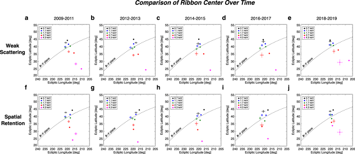
Figure 10. Time series of the ribbon center as a function of energy from the weak scattering ribbon model (a)–(e) and spatial retention ribbon model (f)–(j) compared to the IBEX ribbon-separated data (open circles with uncertainties).
Download figure:
Standard image High-resolution image
Figure 11. Time series of the ribbon radius as a function of energy from the weak scattering ribbon model (a)–(e) and spatial retention ribbon model (f)–(j) compared to the IBEX ribbon-separated data (open circles with uncertainties).
Download figure:
Standard image High-resolution imageAs shown in Figure 10, both models and the data ribbon centers' exhibit a large spread in latitude of ribbon centers as a function of ENA energy, with centers at larger energies observed at lower latitudes. The centers of the ribbon-separated results from spherical harmonic decomposition (Swaczyna et al. 2022) are qualitatively similar to earlier analyses of determining the ribbon center from the total ENA flux in the sky (Funsten et al. 2013; Dayeh et al. 2019), in terms of the trend in latitude as a function of energy. It is also consistent with the theoretical model of the ribbon centers from Swaczyna et al. (2016), who showed that the latitudinal asymmetry of the SW speed likely creates the spread in latitude of the ribbon centers as a function of ENA energy.
Dayeh et al. (2019) performed the first analysis of the time-dependent evolution of the IBEX ribbon centers, which we compare to here. Again, while qualitatively similar, the change in observed ribbon centers from our current analysis over time is much more significant than the results from Dayeh et al. (2019), presumably due to the ribbon separation before performing the circle fitting. Without ribbon separation prior to fitting, Dayeh et al. (2019) show that the ribbon centers do not significantly change over time, within their 1σ uncertainties (see their Figure 6). We also note that the ribbon center uncertainties from Dayeh et al. (2019) were assumed to be the same as the radius uncertainties, which are typically larger than our center uncertainties, which are derived from the minimized chi-square deviates. In our analysis, we see more significant changes over time in both models and the data results. For example, the latitudinal spread in centers is largest in 2009–2011 and 2018–2019, and in 2014–2015 the data show a clockwise rotation in the ribbon centers compared to other years. The data in 2009–2011 and 2018–2019 reflect solar minimum conditions (with fast SW at high latitudes and slow SW at low latitudes), while in 2014–2015 the SW conditions were more symmetric in latitude. Zirnstein et al. (2016a) showed that, under the assumption of uniform SW speed in latitude, the ribbon centers do not show significant spread in latitude, but rather become more aligned with the B - V plane. This explanation appears consistent with the data results shown in Figures 10(c) and (h) in 2014–2015. Thus, it appears that the ribbon centers as a function of energy, when derived after separating the ribbon signal from the GDF, do change over time and reflect the SW latitudinal characteristics over the solar cycle.
The modeling results show similarities to the data, although there are significant departures in 2014–2017 for the weak scattering model, especially at 2.7–4.3 keV. The spatial retention model better reproduces the data, but there is an almost time-independent, systematic ∼2°–3° shift in the model centers from the data along the B – V plane. It is possible that, with the larger plasma grid size in the current simulation (with radius 2500 au compared to 1000 au in Zirnstein et al. 2016b), the draping of the ISMF around the heliosphere is slightly different. We have determined that more ENAs from the heliotail in our 2500 au simulation are able to travel upstream of the heliopause and slightly modify the plasma conditions upstream of the bow wave by slightly increasing the temperature. This may then slightly alter way the ISMF is compressed and draped in the ribbon source region. While this effect appears small (a few degrees), this will be the subject of a future investigation.
Figure 11 shows the ribbon radius as a function of ENA energy and time for the models and data. In general, the weak scattering model results are qualitatively similar to the data results, but the model systematically overestimates the observed ribbon radius by a few degrees. As explained by Zirnstein et al. (2021a), the reason why the weak scattering model produces a larger ribbon radius is because the mean ENA source distance is farther from the heliopause than in the spatial retention model. Zirnstein et al. (2021a) explained that, in order to fix this discrepancy, the pristine ISMF magnitude would need to decrease by ∼1 μG, which is a significant change and highly unlikely to be realistic. The spatial retention model compares very well to the data at all energies and times. The observed ribbon radius at 4.3 keV in 2018–2019 is smaller by almost 4° than the spatial retention model, but we note that the separated ribbon at 4.3 keV has significantly low signal, and uncertainties in the fitting procedure may not be accounted for in these plots. Therefore, we believe the spatial retention model of the ribbon radius overall agrees with the observations.
While the ribbon centers and radii show significant evolution in time for different ENA energies, Figure 12 demonstrates that the energy-averaged center and radius of the ribbon do not significantly change over time. Both the models and the data average center results lie on or close to the B – V plane, consistent with our previous analysis showing that the average ribbon center lies along the same plane defined by interstellar magnetic field B and the LISM inflow vector V far from the heliosphere (nominally chosen at 1000 au; Zirnstein et al. 2016b). There are only slight differences between the weak and strong scattering model centers, but a significant difference in their radii, as explained earlier. The observed ribbon centers do not appear to change over time, within uncertainties, and the spatial retention model results lie within the observed radius uncertainties over the solar cycle. We note that the energy average does not include ESA 6 results, because the fitting analysis of the observations did not yield meaningful results from 2012 to 2017, due to the culling criteria as described in the Appendix (which mostly affected ESA 6), and therefore we left out ESA 6 from the averages in both models and the data.

Figure 12. Time series of energy-averaged ribbon center (a, c) and radius (b, d), comparing both models (filled circles) with the data (open circles with uncertainties). It should be noted that, because we do not have results for IBEX ESA 6 data in 2012–2017, and systematic uncertainties in the analysis in fitting the ribbon at ESA 6 are likely unaccounted for, we do not include ESA 6 results in the average over energy.
Download figure:
Standard image High-resolution image4. Conclusions
The IBEX ribbon, which is formed by the secondary ENA mechanism, has characteristics that can inform us about the large-scale interaction of the heliosphere with the LISM, e.g., properties of the ISMF draped around the heliosphere, as well as small-scale particle dynamics describing the behavior of energetic PUIs in the LISM before they become secondary ENAs, e.g., the rate of particle pitch angle scattering and retention near B · r = 0. Following some of our previous work, we have implemented two simplified scenarios for particle pitch angle scattering: (1) "weak scattering", where particles are free to stream along the local ISMF before experiencing charge exchange, and (2) "spatial retention," a form of strong pitch angle scattering proposed by Schwadron & McComas (2013) that enhances PUI densities near B · r = 0 in bispherical distributions. Implementing these two limiting scenarios of scattering in a global MHD model of the heliosphere, with an evolving neutral SW and PUI source distribution, yielded results for the energy-dependent intensity and geometric properties of the ribbon evolving over time that, when compared with IBEX observations, revealed intriguing conclusions about the source of the IBEX ribbon.
First, we showed that the evolution of the IBEX ribbon is largely reproduced over the past solar cycle by both of our models when a time-dependent source of neutral SW and neutral PUI is included (Figures 3–4). However, the intensity of the ribbon modeled under the spatial retention mechanism greatly underestimates IBEX observations when implemented in a global MHD model, contrary to predictions by Schwadron & McComas (2013). This is not a completely new result (Zirnstein et al. 2021a), and it highlights the need for potential modifications of the spatial retention theory in order to enhance the ribbon intensity over all energies, such as by forming a more anisotropic distribution of PUIs outside the heliopause with pitch angles closer to 90° in the retention region. It is possible that such a modification to the spatial retention model may change the geometric properties of the resulting ribbon. This will depend on whether the ribbon source distribution as a function of distance from the heliopause is significantly changed. However, we do not expect that this modification will result in changes as large as the differences between the spatial retention and weak scattering models, which are significantly different from each other in terms of how the ribbon source is distributed in space (Zirnstein et al. 2018, 2019a).
Nevertheless, both the weak scattering and spatial retention models qualitatively reproduce the evolution of the IBEX data in most parts of the sky, as shown in Figure 9. Some differences are likely due to inaccuracies of the SW speeds derived from IPS observations. Moreover, the inclusion of neutralized interstellar PUIs is essential for reproducing IBEX data at energies >2 keV, because the neutral PUI source dominates the ribbon signal at these energies (Figures 5–6). We implemented a neutral PUI source, based on New Horizons' SWAP observations of interstellar PUIs (McComas et al. 2021), to provide the most accurate representation of their distribution as a function of distance from the Sun.
We also showed that the evolution of the ribbon's center location and radius as a function of ENA energy is sensitive to the pitch angle scattering assumptions of our models. We find that there is significant spread of the ribbon centers in latitude depending on ENA energy, as reported and modeled in a few previous studies (Swaczyna et al. 2016; Dayeh et al. 2019), but their evolution over time shows moderate changes—especially at higher ENA energies. The spatial retention model compares better to IBEX observations (Figures 10–11) than the weak scattering model for both the ribbon center and radius as a function of energy and time. Both models' ribbon centers are slightly offset from the observations, suggesting the pristine ISMF vector implemented in our global heliosphere model should be shifted along the B - V plane a few degrees toward the nose (Zirnstein et al. 2016b). Moreover, the weak scattering model ribbon radius overestimates the observed ribbon radius consistently by a few degrees, indicating it would need a significantly weaker ISMF to compensate (by ∼1 μG). A decrease by 1 μG is very significant and would change the total LISM pressure outside the heliopause (Pogorelov et al. 2011; Schwadron et al. 2011) and the LISM densities as we currently know them (Bzowski et al. 2019; Zirnstein et al. 2021a). But this is not required for the spatial retention model, thus providing the ribbon radius as a reliable observable to differentiate these two models. Exactly how much of a change of the LISM parameters would be required in order to force the weak scattering model to match the geometry of the observed ribbon should be examined in a future study.
While the position of the ribbon center and its radius changes over time for separate ESAs, the energy-averaged properties do not significantly change over time (Figure 12) and are well reproduced by the spatial retention model. This might indicate that any Rayleigh–Taylor or Kelvin–Helmholtz instabilities that may exist at the heliopause would not fluctuate significantly over times smaller than a solar cycle (Borovikov & Pogorelov 2014; Pogorelov et al. 2017). This is an especially important finding if the IBEX ribbon is produced via spatial retention, where the ribbon source region is on average closer to the heliopause than the weak scattering ribbon source region (Zirnstein et al. 2018, 2019a).
Thus, we conclude, with our most sophisticated model of the IBEX ribbon to date, that the spatial retention model of the ribbon is a more favorable scenario for explaining the ribbon in terms of temporal evolution and geometric properties. However, as stated earlier, the ribbon intensity from this model greatly underestimates the observations (by a factor of ∼4) and needs further improvements to better understand the particle dynamics in the retention region. We hypothesize that scattering by magnetic mirroring near B · r = 0 as demonstrated by Giacalone & Jokipii (2015, 2020) and Zirnstein et al. (2020a) may yield more anisotropic PUI distributions with pitch angles closer to 90° and might increase ribbon ENA fluxes observed at 1 au. The enhanced PUI density near B · r = 0 and the proximity of the ribbon source region to the heliopause in the spatial retention model are crucial to its observed geometry, which might change if the mechanism of scattering is altered.
Nevertheless, the positive comparison between the model and data also support that (1) the ribbon is indeed formed from the secondary ENA mechanism, and that (2) the ISMF derived by Zirnstein et al. (2016b), which was implemented in our current global MHD model, is still a reasonably accurate measure of the ISMF in the pristine LISM. In a future study, we plan to develop more accurate intensities of the ribbon under the spatial retention mechanism, in the hope of better reproducing IBEX observations. Improvements to our models will also be useful for analyzing higher-sensitivity and higher-resolution measurements of the ribbon made by the Interstellar Mapping and Acceleration Probe (IMAP; McComas et al. 2018a), which is expected to launch in 2025.
This work was supported by NASA's Heliophysics Guest Investigators—Open program under grant No. 80NSSC21K0582. E.J.Z. also acknowledges partial support from the Laboratory Directed Research and Development program of Los Alamos National Laboratory under sponsor award No. CW18805, and partial support for past development of the ribbon models under NASA's Heliophysics Supporting Research program under grant No. 80NSSC17K0597.
Appendix
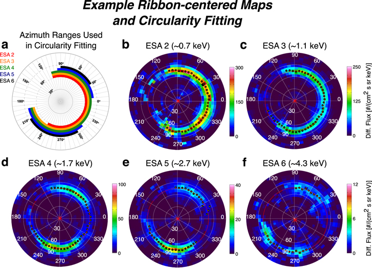
The procedure for determining the center location and radius of the ribbon is based on methods used by Dayeh et al. (2019) and Zirnstein et al. (2021a), which we summarize here. The same procedure is applied to the separated ribbon data and the models, with some minor differences. First, a Gaussian function of the following form is fit to the ribbon peak in each azimuthal sector in a ribbon-centered frame:

where  is the ribbon flux as a function of the polar angle from the ribbon center plot, θ, the 6° azimuthal sector angle around the polar frame, ϕ, the time period of the data/model results, t, and the ESA passband energy, E. The fit parameters are: (1) A, the peak flux above the background (which is zero for these ribbon-only maps), (2) θc
, the polar angle of the ribbon peak from the center, and (3) σG
, the 1σ width of the Gaussian fit to the ribbon. Equation (A1) is fit to the separated ribbon IBEX data that are first weight-averaged over five time periods: 2009–2011, 2012–2013, 2014–2015, 2016–2017, and 2018–2019. The same equation is fit to the models for each yearly map while taking into account the IBEX's observation times during its Sun-pointing axis spin and orbit around the Sun over the course of each year. We do not fit Equation (A1) to azimuthal sectors near the heliotail and magnetosphere. The ranges we exclude are different for each ESA, as illustrated in Figure 13 and listed here (ranges go counterclockwise and include pixel edges): 8°–240° (ESA 2), 108°–192° (ESA 3 and 4), 96°–192° and 312°–6° (ESA 5), and 90°–210° and 300°–30° (ESA 6). The same ranges are then applied to the models. Equation (A1) is fit using Levenberg–Marquardt chi-square minimization, where data uncertainties are used as weights in the fitting. Because the model results do not have uncertainties, but the fitting procedure may be sensitive to the amplitude of flux across the ribbon, we assume model uncertainties are proportional to
is the ribbon flux as a function of the polar angle from the ribbon center plot, θ, the 6° azimuthal sector angle around the polar frame, ϕ, the time period of the data/model results, t, and the ESA passband energy, E. The fit parameters are: (1) A, the peak flux above the background (which is zero for these ribbon-only maps), (2) θc
, the polar angle of the ribbon peak from the center, and (3) σG
, the 1σ width of the Gaussian fit to the ribbon. Equation (A1) is fit to the separated ribbon IBEX data that are first weight-averaged over five time periods: 2009–2011, 2012–2013, 2014–2015, 2016–2017, and 2018–2019. The same equation is fit to the models for each yearly map while taking into account the IBEX's observation times during its Sun-pointing axis spin and orbit around the Sun over the course of each year. We do not fit Equation (A1) to azimuthal sectors near the heliotail and magnetosphere. The ranges we exclude are different for each ESA, as illustrated in Figure 13 and listed here (ranges go counterclockwise and include pixel edges): 8°–240° (ESA 2), 108°–192° (ESA 3 and 4), 96°–192° and 312°–6° (ESA 5), and 90°–210° and 300°–30° (ESA 6). The same ranges are then applied to the models. Equation (A1) is fit using Levenberg–Marquardt chi-square minimization, where data uncertainties are used as weights in the fitting. Because the model results do not have uncertainties, but the fitting procedure may be sensitive to the amplitude of flux across the ribbon, we assume model uncertainties are proportional to  . Additional constraints we apply to the data (not the models) for each azimuthal sector are: (1) the derived ribbon peak position from the center must be between 60° and 90°; (2) the peak location uncertainty must be less than the peak location; (3) the peak ribbon flux uncertainty must be less than the peak ribbon flux; (4) for ESA 6, at least three points must be available in each 30° azimuthal section, to ensure wide enough coverage for fitting a circle.
Figure 13. Examples of ribbon-centered maps and circularity analysis results. (a) Azimuth ranges used in the circle fitting procedure for ESA 2–6. (b–f) IBEX ribbon-separated data from Swaczyna et al. (2022) averaged over 2009–2011 for ESA 2–6, showing the ribbon peak positions from the Gaussian fitting (black dots; uncertainties shown as yellow lines) and circle fits to the ribbon peaks (red circles). The ribbon centers are shown as red asterisks.
Download figure:
Standard image High-resolution image
After the fits to find the ribbon peak position, its 1σ width, and their uncertainties, we fit a circle to the ribbon peaks in order to find the ribbon center and radius via minimization of chi-square in the following form (Swaczyna et al. 2016):

where  is the ribbon center in ecliptic J2000 latitude and longitude, r is the mean ribbon radius, the function
  converts the ribbon center between ecliptic J2000 and ribbon-center frame coordinates and finds the angle distance from the center, and σi
is the uncertainty of the peak position. The uncertainties of the resulting longitude and latitude of the ribbon center are calculated from the summation over deviates of the minimized chi-square, and then scaled by the square root of the reduced chi-square under the assumption that the ribbon can be described by a Gaussian function. The uncertainty of the radius is calculated from the unweighted standard deviation of the peak positions of the ribbon from the mean ribbon radius, divided by
converts the ribbon center between ecliptic J2000 and ribbon-center frame coordinates and finds the angle distance from the center, and σi
is the uncertainty of the peak position. The uncertainties of the resulting longitude and latitude of the ribbon center are calculated from the summation over deviates of the minimized chi-square, and then scaled by the square root of the reduced chi-square under the assumption that the ribbon can be described by a Gaussian function. The uncertainty of the radius is calculated from the unweighted standard deviation of the peak positions of the ribbon from the mean ribbon radius, divided by  , yielding the unweighted standard error. However, the final uncertainties of the model are not meaningful, because the model fluxes do not have uncertainties; therefore, we do not plot them in Figures 10–12.