


Abstract
We analyze proton bulk parameters derived from Ulysses observations and investigate the polytropic behavior of solar wind protons over a wide range of heliocentric distances and latitudes. The large-scale variations of the proton density and temperature over heliocentric distance indicate that plasma protons are governed by subadiabatic processes (polytropic index γ < 5/3), if we assume protons with three effective kinetic degrees of freedom. From the correlation between the small-scale variations of the plasma density and temperature in selected subintervals, we derive a polytropic index γ ∼ 1.4 on average. Further examination shows that the polytropic index does not have an apparent dependence on the solar wind speed. This agrees with the results of previous analyses of solar wind protons at ∼1 au. We find that the polytropic index varies slightly over the range of the heliocentric distances and heliographic latitudes explored by Ulysses. We also show that the homogeneity of the plasma and the accuracy of the polytropic model applied to the data points vary over Ulysses' orbit. We compare our results with the results of previous studies that derive the polytropic index of solar wind ions within the heliosphere using observations from various spacecraft. We finally discuss the implications of our findings in terms of heating mechanisms and the effective degrees of freedom of the plasma protons.
Export citation and abstract BibTeX RIS

Original content from this work may be used under the terms of the Creative Commons Attribution 4.0 licence. Any further distribution of this work must maintain attribution to the author(s) and the title of the work, journal citation and DOI.
1. Introduction
The polytropic equation (e.g., Chandrasekhar 1967) describes the correlation between the density n and the temperature T (or pressure P ∝ nT) of a fluid, through the polytropic index γ

The polytropic equation becomes vital in space plasma studies, as it brings closure to the hierarchy of the plasma moments (e.g., Kuhn et al. 2010). Additionally, the use of the polytropic relationship can simplify the studies of complicated mechanisms, including energy transfer between particles and fields (e.g., Kartalev et al. 2006). More specifically, the value of γ is indicative for the energy transfer involved in the observed process and the effective degrees of freedom f of the plasma particles. For example, during an adiabatic process, there is no heat transfer during the plasma compression or expansion. In this case, the polytropic index is equal to the ratio of the specific heats  , and is related to the kinetic degrees of freedom of the plasma particles f, such as
  . For instance, γ = 5/3 corresponds to adiabatic plasma particles with three kinetic degrees of freedom (f = 3). In another special case, an isothermal process (constant T) is characterized by γ = 1. During this process, the energy supplied to the system as heat balances the energy supplied to the system as work. Additionally, γ = 0 corresponds to isobaric plasmas (constant P) and γ = ∞ to isochoric plasmas, in which n is constant (for more see Livadiotis 2016, 2019; Nicolaou et al. 2020). Therefore, γ is a useful tool we can use to understand the nature of physical plasma mechanisms without solving complicated energy equations (e.g., Bavassano et al. 1996). Interestingly, although space plasmas are generally only very weakly collisional, we can describe some of their aspects using the fluid description and the polytropic equation, over a wide range of timescales (Verscharen et al. 2019; Wu et al. 2019; Coburn et al. 2022).
Several studies apply the polytropic model to particle observations in planetary magnetospheres. For example, Arridge et al. (2009) fit a polytropic model to electron observations obtained by Cassini in Saturn's magnetotail plasma sheet. Their analysis shows that the electrons in the specific region exhibit an isothermal behavior. Dialynas et al. (2018) use Cassini observations to derive the energetic ion moments in Saturn's magnetosphere. The authors then apply a polytropic model to the derived density and temperature, revealing different behaviors for the observed species within the explored region. Nicolaou et al. (2014a, 2015) derive the bulk parameters of plasma protons in the deep Jovian magnetotail using observations by New Horizons and identify intervals with anticorrelated n and T. Linear log10(T) versus log10(n) fits to these intervals determine an isobaric relationship, indicating that the spacecraft crossed streamlines that were in pressure balance, or streamlines with plasma with isobaric behavior (γ = 0). In another study, Park et al. (2019) use observations by the Time History of Events and Macroscale Interactions during Substorms (THEMIS) mission to identify intervals where the plasma n and T are correlated. The analysis of these intervals makes it possible to calculate the polytropic index of ions in the magnetosheath of Earth and finds that γ varies with the bow-shock geometry.
Numerous other studies investigate the polytropic behavior of solar wind plasma in the inner heliosphere including at ∼1 au. For instance, Totten et al. (1995) use Helios observations to derive empirical relationships describing the proton density and temperature as functions of the heliocentric distance. These relationships determine a subadiabatic behavior (γ ∼ 1.46) on average. In another study, Newbury et al. (1997) use Pioneer Venus Orbiter (PVO) measurements in the vicinity of stream interaction regions. They show a strong correlation between the proton n and T, which determines an adiabatic polytropic index γ ∼ 5/3, and occasionally γ ∼ 2, suggesting that the degrees of freedom may be restricted. Kartalev et al. (2006) evaluate the Bernoulli integral fluctuations in the solar wind in order to select suitable time intervals for further analysis to estimate γ of solar wind protons and electrons at ∼1 au. The study by Nicolaou et al. (2014b) uses a similar method to analyze proton observations obtained from multiple spacecraft at ∼1 au, between 1995 January 1 and 2012 June 30. Their analysis derives an average γ ∼ 1.8. The authors discuss the variations of γ as a function of the solar activity, as well as possible biases due to the instrument providing the observations. Several analyses of Wind spacecraft observations employ a very similar method to characterize the polytropic behavior of solar wind protons at ∼1 au (e.g., Livadiotis & Desai 2016; Livadiotis 2018a; Nicolaou & Livadiotis 2019; Nicolaou et al. 2021a, 2021b; Livadiotis & Nicolaou 2021). These analyses calculate a nearly adiabatic plasma with γ ∼ 5/3 on average. Moreover, the results show that γ does not depend on the plasma speed or the solar activity. Recently, Nicolaou et al. (2020) analyzed high-time-resolution observations of Solar Wind protons by Parker Solar Probe (PSP), revealing large-scale variations characterized by γ ∼ 5/3 and short-timescale fluctuations with γ ∼ 2.7. The authors discuss possible mechanisms that restrict the effective degrees of freedom or involve energy transfer from/to the plasma.
The analyses of measurements in the outer heliosphere offer unique opportunities to study the evolution of the solar wind behavior as it propagates away from the Sun. For example, Elliott et al. (2019) analyze solar wind proton observations by New Horizons, obtained in the heliocentric distance range spanning from 21 to 43 au. A linear fitting to log10(T) and log10(n) in selected time subintervals calculates the variation of γ over heliocentric distance. Those authors found that γ approaches ∼0 (isobaric process) in the outer heliosphere. Interestingly, analyses of Interstellar Boundary Explorer (IBEX) observations determine γ ∼ 0 for the ion plasma in the inner heliosheath (e.g., Livadiotis et al. 2011; Livadiotis & McComas 2013; Livadiotis et al. 2013, 2022).
A complete understanding of the solar wind polytropic behavior within the entire heliosphere requires the analysis of measurements obtained across multiple locations throughout the system. In this study, we analyze Ulysses observations that are obtained over a range of heliocentric distances—and importantly, almost all heliographic latitudes. We explore whether the plasma is described with a polytropic relationship and if this relationship depends on the plasma speed, heliocentric distance, and/or heliographic latitude. In Section 2, we describe the proton parameters we use for our analyses. In Section 3, we describe our methodology. In Section 4, we show our results, which we discuss extensively in Section 5.
2. Data
Figure 1 shows the spacecraft attitude information and plasma parameters we analyze in this study. Among the spacecraft heliocentric distance R and heliographic latitude Θ, we use the 4 min resolution proton bulk parameters, which are derived by fitting Solar Wind Observations Over the Poles of the Sun (SWOOPS) observations (Bame et al. 1992) to bi-Maxwellian core-beam distributions. Although the fitting is applied to the entire proton distribution observed within the instrument's energy range, here we use only the slow population parameters, which normally correspond to the proton core. In the Appendix, we verify the results by applying an additional data filter based on the density ratio of the two populations. The details for the fit parameters are found at spase://NASA/NumericalData/Ulysses/SWOOPS/Proton/FitParameters/PT4M. For our analysis, we specifically use the proton core density n, scalar temperature T, flow speed V, and Alfvén speed  , where B is the magnetic field, ρ is the mass density, and μ0 is the permeability constant. The scalar temperature T is calculated from the thermal speeds parallel and perpendicular to the magnetic field Vth,∥ and Vth,⊥, respectively, such as
 ![$T=\tfrac{1}{3}\left[\tfrac{1}{2}{m}_{{\rm{p}}}{V}_{\mathrm{th},\parallel }^{2}+{m}_{{\rm{p}}}{V}_{\mathrm{th},\perp }^{2}\right]$](https://content.cld.iop.org/journals/0004-637X/948/1/22/revision1/apjacbf33ieqn4.gif) , where mp is the mass of the proton. We analyze the time period spanning from 1992 January 1 to 1998 December 31, which is a period of minimum solar activity, during which the solar wind is well structured as a function of the heliographic latitude (see McComas et al. 1998, 2008). As shown in Figure 1, during the analyzed time period, most of the fast solar wind (V > 600 km s−1) is observed at high absolute heliographic latitudes (
, where mp is the mass of the proton. We analyze the time period spanning from 1992 January 1 to 1998 December 31, which is a period of minimum solar activity, during which the solar wind is well structured as a function of the heliographic latitude (see McComas et al. 1998, 2008). As shown in Figure 1, during the analyzed time period, most of the fast solar wind (V > 600 km s−1) is observed at high absolute heliographic latitudes ( > 40°).
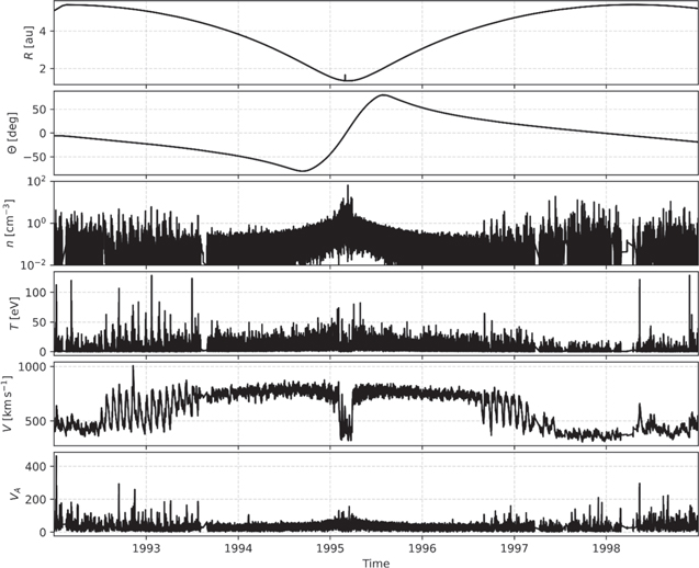
Figure 1. Time series of parameters we use in our analysis. From top to bottom, we show the heliocentric distance of the spacecraft R, its heliographic latitude Θ, the plasma core density n, temperature T, bulk flow speed V, and Alfvén speed VA .
Download figure:
Standard image High-resolution image3. Methodology
3.1. Histograms of Large-scale Variations
Similarly to Nicolaou et al. (2020), we first examine the large-scale variations of the plasma density and temperature as functions of the heliocentric distance by constructing the 2D histograms of log10(n) versus  and log10(T) versus
  , respectively. The resolutions we use for these histograms are
  ×
×  = 0.075 × 0.01 and
  ×
×  = 0.05 × 0.01, respectively. Further, we normalize each column of these histograms to the maximum occurrence recorded within the specific
  bin. As explained in Livadiotis & Desai (2016), and later on in Livadiotis (2018b) and Nicolaou et al. (2020), when there are not extreme values in the sampled data set, this normalization brings all the columns to the same level of occurrence and the correlation between the examined parameters becomes clearer. We then examine the correlation between the large-scale variations of the plasma density and temperature by constructing the 2D histogram of log10(T) versus log10(n) with resolution
  ×
×  = 0.05 × 0.075. Again, because there are no extreme values in our samples, in order to reveal the correlation between the two parameters, we normalize the occurrence values in each log10(T) bin (each column) to the maximum occurrence recorded within the bin.
3.2. Linear Fits to Short-scale Variations
To investigate the short-timescale variations of n and T and identify their correlation, we divide the entire data set spanning from 1992 January 1 to 1998 December 31, in subintervals of eight consecutive data points. This method groups the data into ∼360,000 subintervals, with the first subinterval containing the 1st–8th data points of the original time series, the second interval containing the 2nd–9th data points, and so on. Due to nonuniform gaps in the data, the duration of the subintervals varies. In Figure 2, we show the histogram of the duration of the subintervals we analyze in this study. The longest subinterval we analyze does not exceed 200 minutes.

Figure 2. Histogram of the analyzed subinterval length.
Download figure:
Standard image High-resolution imageFollowing a methodology similar to those of other studies deriving the polytropic index from single-spacecraft observations, we perform a linear regression to log10(T) versus log10(n) within each subinterval (e.g., Newbury et al. 1997; Arridge et al. 2009; Livadiotis 2018a, 2018b; Nicolaou et al. 2021a, 2021b, 2021c). The slope of the fitted lines determines γ because, according to Equation (1):

For each subinterval, we calculate the Pearson correlation coefficient of log10(T) versus log10(n) and the residuals between the data points and the fitted line. We use these parameters to evaluate the applicability of the polytropic model to the observations. We also calculate the standard deviation and the mean value of the Bernoulli integral in each subinterval. We use the Bernoulli integral (BI) for an adiabatic plasma (γ = 5/3):

which is a reasonable simplification in our case, as we discuss in the Appendix. The ratio of the standard deviation of the Bernoulli integral over its mean value  within each analyzed subinterval is proportional to the homogeneity of the analyzed plasma and indicates whether the data points we analyze correspond to the same streamline or not (e.g., Kartalev et al. 2006; Nicolaou et al. 2014b; Pang et al. 2015; Livadiotis 2018a, 2018b; Nicolaou et al. 2021a, 2021b). In Figure 3, we show three examples of such subintervals; one with γ ∼ 5/3, another with γ ∼2, and another with γ ∼ 1.2. All subintervals shown in Figure 3 exhibit a strong linear correlation (Pearson coefficient > 0.9) between log10(T) and log10(n), and they have a
  ratio <3%.
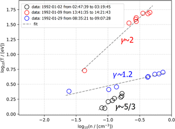
Figure 3. Three subintervals of log10(T) vs. log10(n). Each set of colorful circles are data points within subintervals exhibiting a strong correlation between log10(T) vs. log10(n) (Pearson coefficient > 0.9), while the gray dashed lines are fitted linear models to the data. Black data points correspond to an interval that is described with γ ∼5/3, while red data points are fitted with γ ∼ 2, and blue data points with γ ∼ 1.2.
Download figure:
Standard image High-resolution image4. Results
4.1. Large-timescale Variations
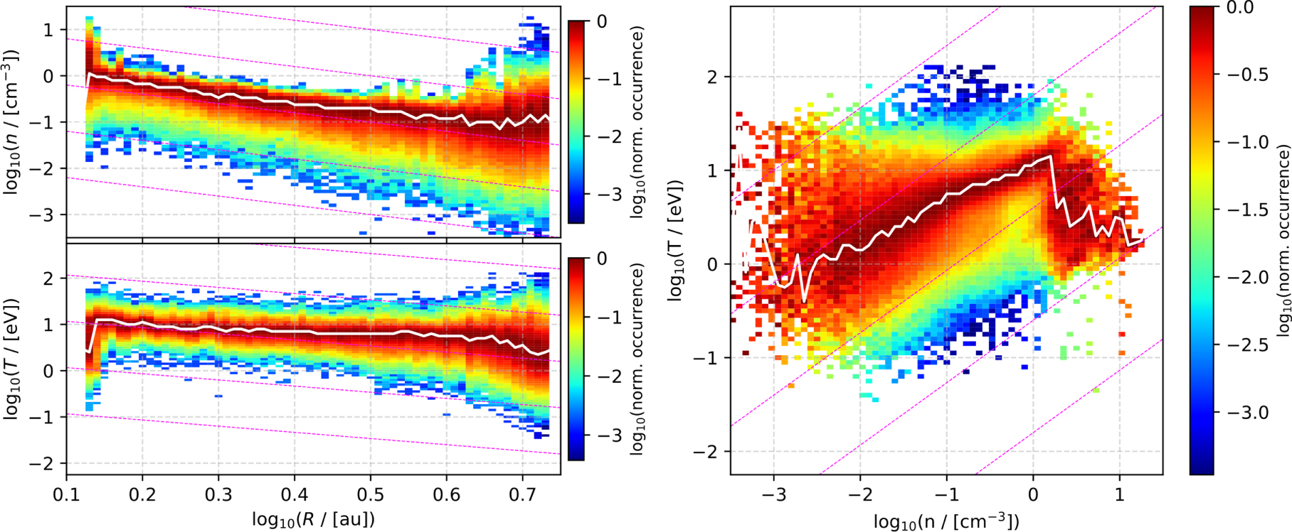
In the top left panel of Figure 4, we show the 2D histogram of log10(n) versus  . The magenta lines on the same panel show the relationship n ∝ R−2, which describes the spherical expansion of steady-speed plasma. Our result does not show any apparent deviation from the spherical expansion model for 1.38 au < R < 4 au (
 ). For R < 1.38 au and R > 4 au, the density is larger than the overall trend. This is expected because, at these heliocentric distances, Ulysses observes low-latitude regions (
 < 40°; see Figure 1), which are sources of denser plasmas, as shown in McComas et al. (2000).

Figure 4. Large-scale variations of plasma density and temperature. (Top left) Two-dimensional histogram of log10(n) vs.  . The magenta lines show the n ∝ R−2 relationship. (Bottom left) Two-dimensional histogram of log10(T) vs.
  . The magenta lines on the same panel show the relationship T ∝ R−4/3. (Right) Two-dimensional histograms of log10(T) vs. log10(n), while the magenta lines in the same panel show the relationship T ∝ n2/3. The white lines in each panel correspond to the maximum occurrence in each column of the corresponding histogram.
Download figure:
Standard image High-resolution imageThe bottom left panel of Figure 4 shows the corresponding 2D histogram of log10(T) versus  . According to the polytropic relationship in Equation (1) and for n ∝ R−2, the radial profile of the plasma temperature is
  . The magenta lines on the same panel show the relationship T ∝ R−4/3, which is the expected temperature profile for adiabatic plasma with three degrees of freedom (γ = 5/3). For most of the R range we examine here, the profile of the solar wind proton temperature is less steep than the magenta lines. More specifically, our observation is consistent with the expansion of a subadiabatic plasma (
 ). During an adiabatic expansion, the work done by the expanding gas (dw ≡ PdV) is balanced by the reduction of the internal energy (dU ≡ cv
dT), so that dq ≡ dU + dw = 0. The observed temperature profile, however, indicates that the internal energy reduction is not sufficient to balance the work done by the gas, which expands with n ∝ R−2. As we discuss further in Section 5, this observation implies that new energy is possibly supplied by external mechanism(s) to solar wind protons. This agrees with Richardson & Smith (2003), who construct the radial temperature profile of the protons, using Voyager observations within 1 au < R < 70 au. In Section 5, we discuss possible heating mechanisms that can result in the observed proton core temperature profile. Finally, for R < 1.38 au and R > 4 au, the temperature is lower than the overall trend. As mentioned above, at these radial distances, Ulysses observed plasmas originating from low-latitude regions. As shown in McComas et al. (2000), low-latitude regions are sources of colder (and denser) plasmas. Therefore, the deviation of the overall temperature profile in this R range is not related to the polytropic behavior.
). During an adiabatic expansion, the work done by the expanding gas (dw ≡ PdV) is balanced by the reduction of the internal energy (dU ≡ cv
dT), so that dq ≡ dU + dw = 0. The observed temperature profile, however, indicates that the internal energy reduction is not sufficient to balance the work done by the gas, which expands with n ∝ R−2. As we discuss further in Section 5, this observation implies that new energy is possibly supplied by external mechanism(s) to solar wind protons. This agrees with Richardson & Smith (2003), who construct the radial temperature profile of the protons, using Voyager observations within 1 au < R < 70 au. In Section 5, we discuss possible heating mechanisms that can result in the observed proton core temperature profile. Finally, for R < 1.38 au and R > 4 au, the temperature is lower than the overall trend. As mentioned above, at these radial distances, Ulysses observed plasmas originating from low-latitude regions. As shown in McComas et al. (2000), low-latitude regions are sources of colder (and denser) plasmas. Therefore, the deviation of the overall temperature profile in this R range is not related to the polytropic behavior.
The right panel of Figure 4 shows a 2D histogram of log10(T) versus log10(n). The correlation of the two parameters confirms that, in general, the proton plasma is subadiabatic. With the magenta lines, we show the relationship T ∝ nγ−1 for γ = 5/3. Clearly, the slope revealed from the observations is smaller, corresponding to γ < 5/3, exactly as inferred from the temperature radial profile. Additionally, the plot suggests that the slope characterizing the density range spanning from 0.1 cm−3 < n < 1 cm−3 is smaller than the slope characterizing the data in the n < 0.1 cm−3 range. Finally, there is a sudden decrease in temperature for n > 1 cm−3, which corresponds to the equatorial flows of slower, denser, and colder solar wind as we discuss above (see also McComas et al. 2000). In the next subsection, we show the calculated behavior of the short-timescale variations.
4.2. Short-timescale Variations
4.2.1. Polytropic Index over Solar Wind Speed
We first examine histograms of the polytropic index we derive from the analysis of short-timescale subintervals (eight consecutive data points) and its correlation with the proton flow speed averaged over each subinterval. The bottom left panel of Figure 5 shows the 2D histogram of γ and V, while the top left panel shows the 1D histogram of V and the right panel shows the 1D histogram of γ. We can identify two peaks in the histogram of V. The first peak, centered at V ∼ 430 km s−1, corresponds to the slow solar wind observed at low latitudes ( < 40°) and the second peak, centered at V ∼ 770 km s−1, corresponds to the fast solar wind that is observed at high latitudes (
 ). However, it should be noted that this structure is very different around solar maximum, when the latitudinal structure of the solar wind breaks down (for more details, see McComas et al. 1998, 2008). The histogram of γ values has only one peak at γ ∼ 1.4. In Figure 6, we show the 2D histogram of γ and V with each column normalized to the maximum occurrence observed in the corresponding V bin. As explained in Section 3.1, after this normalization, a possible correlation between the two parameters is directly revealed, given that there are not extreme values in the data set. In the same panel, we show the mean value of γ (white data points) in each V bin. According to this histogram, there is not any apparent correlation between γ and V. This result agrees with studies of proton plasmas at ∼1 au (e.g., Livadiotis 2018a, 2018b; Nicolaou & Livadiotis 2019) and in the inner heliosphere (e.g., Totten et al. 1995; Nicolaou et al. 2020).

Figure 5. Histograms of γ and V. (Bottom left) Two-dimensional histogram of the polytropic index and the solar wind proton flow speed, (top left) 1D histogram of the proton flow speed, and (right) 1D histogram of the derived polytropic index.
Download figure:
Standard image High-resolution image
Figure 6. Two-dimensional histogram of γ and V, with each column normalized to the maximum occurrence observed in the corresponding V bin. The white data points show the mean value of γ in each V bin. The standard error of the mean values of γ are too small, and therefore are not shown here.
Download figure:
Standard image High-resolution image4.2.2. Polytropic Index over Heliocentric Distance and Heliographic Latitude
In Figure 7, we show 2D histograms of γ and V, for specific R bandwidths with ΔR = 0.5 au. We use the same format as in Figure 6, in terms of normalizing the occurrence and calculating the average value of γ (white data points) and its standard error (error bars), for each V bin. The range of the observed V is different for different R (for a different panel in Figure 7), because the solar wind speed is organized by the latitude, and the latitude observed by the spacecraft orbit is a function of the heliocentric distance. For example, the fast flows in the polar regions are observed only over heliocentric distances between ∼1.75 and ∼4.25 au (see also Figure 1). In general, the plots in Figure 7 confirm that there is not any apparent systematic correlation between γ and V. In Figure 8, we show the mean value of γ and its standard error (error bars), calculated for each R bin (for each panel) shown in Figure 7. According to our result, the polytropic index fluctuates between 1.38 and 1.47 at R < 4.5 au and drops by δγ ∼ 0.1 for R > 4.5 au. We further discuss this result in the next section.
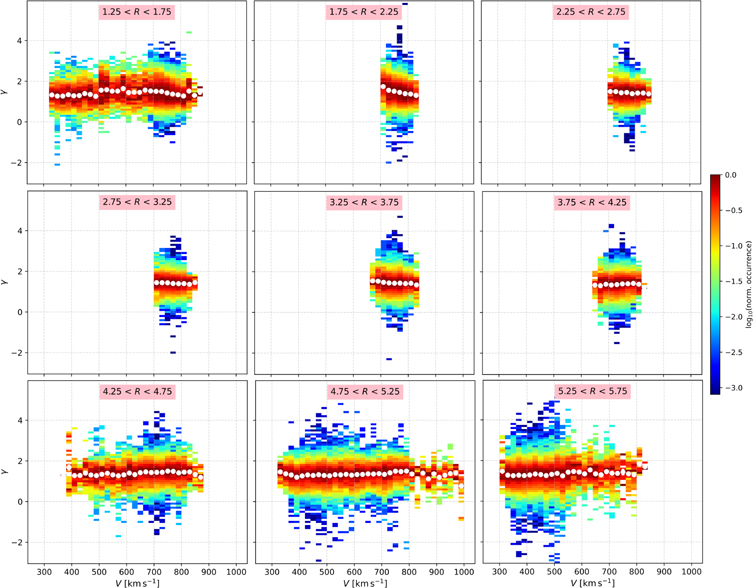
Figure 7. Two-dimensional histograms of γ vs. V at different heliocentric distances. The occurrence in each V bandwidth is normalized to the maximum occurrence value within the V bin. At the top of each panel, we show the heliocentric distance bandwidth that corresponds to the plot.
Download figure:
Standard image High-resolution image
Figure 8. Mean value of γ as a function of the heliocentric distance. The error bars correspond to the standard error of the mean value.
Download figure:
Standard image High-resolution imageIn order to examine a possible dependence of γ on Θ, we plot 2D histograms of γ and V for different Θ bins (Figure 9). Again, there is no evidence for a systematic correlation between γ and V. We then calculate the mean value of γ and its standard error for each Θ bin, which we show in Figure 10. The result indicates that γ increases slightly toward the Sun's poles. The mean value of the polytropic index is γ ± δ γ = 1.45 ± 0.02 at 70° < Θ < 90°, and γ ± δ γ = 1.42 ± 0.02 at −90° < Θ < –70°. However, γ drops to γ ± δ γ = 1.29 ± 0.01 at −10° < Θ < 10°.
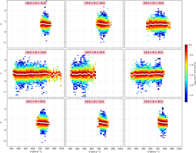
Figure 9. Two-dimensional histograms of γ vs. V at heliographic latitudes. The occurrence in each V band is normalized to the maximum occurrence value within the V bin. At the top of each panel, we show the heliographic latitude band that corresponds to the plot.
Download figure:
Standard image High-resolution image
Figure 10. Mean value of γ as a function of the heliographic latitude.
Download figure:
Standard image High-resolution imageFor completeness, in Figure 11, we show 2D plots of the mean γ and its standard error δγ as functions of R and Θ in a polar coordinate system. For these 2D histograms, we use a resolution δ R × δΘ = 0.25 au × 5°. We can clearly see that the estimated polytropic index decreases slightly with increasing R and for Θ → 0°. Additionally, the plot confirms that γ is slightly higher in the south pole than it is in the north pole. The standard error of γ seems to be higher in the equatorial regions close to the Sun, where the spacecraft was moving fastest and spent the least time, and in mid, positive latitudes away from the Sun.

Figure 11. Two-dimensional plots of (left) mean γ and (right) its standard error, as functions of the heliocentric distance and heliographic latitude.
Download figure:
Standard image High-resolution image4.2.3. Homogeneity and Polytropicity
The polytropic relationship should be determined in analyses of observations of homogeneous plasmas (e.g., Newbury et al. 1997). In other words, the polytropic relationship is applicable in plasmas within the same streamline (e.g., Totten et al. 1995; Kartalev et al. 2006; Nicolaou et al. 2014b; Nicolaou & Livadiotis 2017). As we explain in Section 3.2, we use a simplified method to quantify the homogeneity of the analyzed subintervals through the Bernoulli integral variation, which is based on the method proposed by Kartalev et al. (2006). In the left panel of Figure 12, we show the 2D plot of  , averaged over the R and Θ bins (in the same format as in Figure 11). According to this plot, the mean
  is at its maximum (∼4%) at 1 au <R <2 au and decreases with increasing radial distance. The middle and the right panels of Figure 12 show 2D plots of the Pearson correlation coefficient between
  and
and  and the residuals of the linear fitting we apply to the data within the analyzed subintervals, respectively, in the same format as in Figure 11. Both magnitudes are relevant to the "goodness" of the linear fit of Equation (2) to the data points within each subinterval. Both plots support that the polytropic model describes better the observations obtained closer to the Sun. In Section 5, we discuss these results in much more detail.
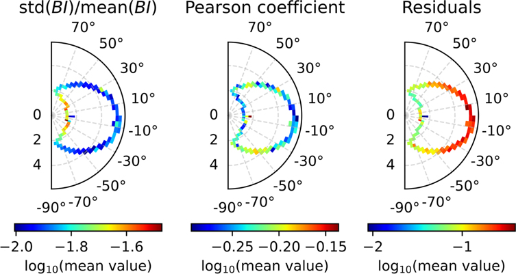
Figure 12. (Left) The relative deviation of the Bernoulli integral within the subintervals we analyze to derive the polytropic index, as a function of the heliocentric distance and the heliographic latitude. (Middle) Pearson correlation coefficient between  and
and  , and (right) fitting residuals between the polytropic model and the data within the analyzed subintervals, both as functions of the heliocentric distance and the heliographic latitude.
Download figure:
Standard image High-resolution image4.2.4. Resolution of Bias Caused by Density Errors
Nicolaou et al. (2019) showed that typical linear fits of Equation (2) to spacecraft observations with statistical uncertainties lead to systematic errors in the calculation of γ. More specifically, statistical uncertainties in the plasma density result in calculations of γ that are artificially closer to the isothermal value (γ = 1). On the other hand, the determination of the special polytropic index,  , by fitting
  versus
  with
with

suffers systematic errors (ν shifting toward 0), depending on the statistical uncertainties of the plasma temperature. The authors propose a method that excludes biased derivations by selecting only the intervals for which the determined γ and ν satisfy

where a is the desired accuracy threshold.
In this section, we would like to verify the discovered trends of γ, using only the intervals that satisfy the criterion in Equation (5). We adopt the suggested data filtering, using a threshold a = 0.25, which selects an appropriate amount of data points to construct reasonable profiles of the mean γ values. Figure 13 shows the determined ν as a function of the determined γ. The dashed line shows  . The blue data points correspond to the derivations that pass the applied filter, while the red data points correspond to derivations that do not.
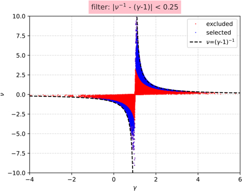
Figure 13. The special polytropic index ν as a function of the polytropic index γ, determined from linear fits to  vs.
vs.  and fitting
  vs.
vs.  observations, respectively. The dashed line shows
  . We apply the filter suggested by Nicolaou et al. (2019), by selecting only data points for which γ is within 0.25 of the definition (blue data points). The red data points are excluded for this test.
Download figure:
Standard image High-resolution imageIn Figure 14(a), we show the 2D histogram of γ and V using the filtered γ values and using the same format as in the bottom left panel of Figure 5. The filter removes a significant number of isothermal values, resulting in a significant decrease of the occurrence at γ = 1. Nevertheless, there is nothing different regarding the most frequent value of γ and its apparent independence of V. In Figures 14(b) and (c), we show the mean γ as a function of R and Θ, respectively. We use the same method as explained in Section 3, but we use only the values that satisfy the applied filter. The profiles of γ verify the behavior of γ shown in Figures 8 and 10. The mean values in Figure 14, however, are slightly larger due to the removal of the isothermal values.
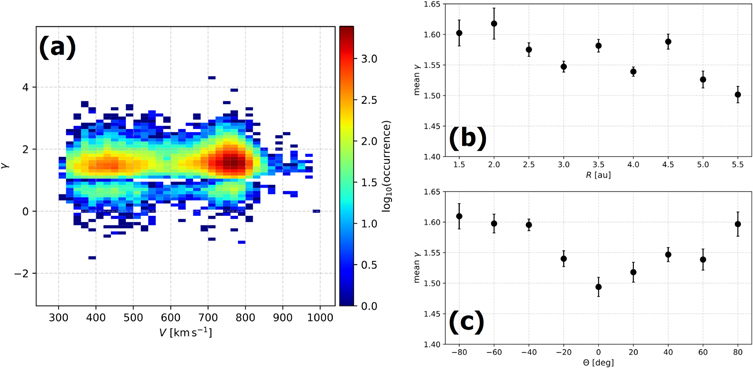
Figure 14. The main results of this study, using only the calculations from the filtered intervals. (a) Two-dimensional histogram of the polytropic index and proton bulk speed. (b) The mean polytropic index as a function of the radial distance and (c) as a function of heliolatidute (see text for details).
Download figure:
Standard image High-resolution image5. Discussion and Conclusions
Observations of solar wind protons, obtained by Ulysses during solar minimum and within the heliocentric distance range from ∼1.5 to ∼5.5 au, support the conclusion that the thermal proton plasma is subadiabatic. The polytropic behavior is evident in both large-scale and small-scale variations of the proton density and temperature. In general, the large-scale variations agree with previous studies in the inner and outer heliosphere. Totten et al. (1995), determined γ ∼ 1.46 for solar wind protons, by characterizing the radial profiles of proton density and temperature observed by Helios between 0.3 and 1 au. Huang et al. (2020) and Nicolaou et al. (2020) used observations by the Parker Solar Probe between 0.27 and 1 au and showed that a subadiabatic model describes the temperature profile reasonably well. Moreover, studies of the thermal (core) proton temperature in the outer heliosphere using observations by Voyager 2 and New Horizons (e.g., Richardson & Smith 2003; Zank et al. 2018) show additional evidence that thermal protons absorb energy as they propagate outward. Richardson & Smith (2003) suggest that thermal protons in the inner heliosphere gain energy (are heated) from stream interaction and/or shocks. In the outer heliosphere, the heating is supplied by pick-up ions. Zank et al. (2018) extends the classical models by Holzer (1972) and Isenberg (1986) to develop a general theoretical model that describes the heating of solar wind thermal protons by low-frequency turbulence, excited by pick-up ions. The radial profiles of the solar wind proton parameters produced by the model are in excellent agreement with the observations.
We attempt to derive γ for individual plasma streamlines by investigating the small-scale fluctuations of n and T. Our small-scale fluctuation analysis determines an average polytropic index γ ∼ 1.4. This is a smaller γ than the one calculated from observations at ∼1 au in previous studies. For instance, Nicolaou et al. (2014b) use observations from multiple spacecraft at ∼1 au and calculate an average proton plasma polytropic index γ ∼ 1.8. Several other studies calculate a nearly adiabatic proton plasma at ∼1 au (e.g., Livadiotis 2018a, 2018b, 2019; Nicolaou & Livadiotis 2019). The more recent study by Nicolaou et al. (2020) uses observations by the Faraday Cup on board Parker Solar Probe and shows that, although the large-scale variations of the plasma density and temperature reveal a nearly subadiabatic plasma, the short-scale variations are characterized with an average γ ∼ 2.7. On the other hand, Elliott et al. (2019) analyze New Horizons observations in the outer heliosphere and show that the proton plasma parameters follow a polytropic behavior with γ ∼ 1.3 at ∼20 au, and γ decreases with radial distance such that γ < 1 for R > 30 au. Livadiotis (2019) combines these results with the results of different studies in the inner and the outer heliosphere to support that the polytropic index decreases gradually from γ ∼ 5/3 at R ∼ 1 au to γ ∼ 0 in the inner heliosheath (e.g., Livadiotis & McComas 2013; Livadiotis et al. 2013).
The results of this study add to our knowledge of the polytropic index value and its variations in the R range from ∼1 to 6 au, as well as over the heliographic latitude. According to our Figure 8, γ decreases by δ γ ∼ 0.1 as the heliocentric distance increases from 4.5 to 5.5 au. In order to increase the statistical accuracy of the data points, in Figure 8, we had to use relatively large R bins (ΔR = 0.5 au). However, the same dependence of γ on R is supported by Figure 11, in which we use smaller R bins (ΔR = 0.25 au), and thus we have more samples of γ over R. Because we do not see a drastic change of γ over the range of R we examine here, we cannot provide accurate estimations of the radial profile of γ. However, if the polytropic index decrement with R is real, then the plasma particle effective degrees of freedom need to increase as the plasma flows outward, or else heat needs to be more effectively provided to the plasma by some mechanism(s) over larger radial distances. This can be realized by considering the relationship between γ, f, the work done by the expanding gas dw, and the heat supplied to the system dq. This relationship (see also Livadiotis 2019) is

If we assume adiabatic protons (dq = 0) for the R range we observe with Ulysses, then  , and the observed trend of γ could be due to f increasing from ∼3 at ∼1 au to ∼7 at ∼6 au. Alternatively, if we consider f = 3 for the distance range we examine, then
  . In this case, there is no significant heat transfer at ∼1 au, but at ∼6 au,
  increases to ∼55%. Our result, combined with the studies by Livadiotis et al. (2013), Elliott et al. (2019), and Livadiotis & McComas (2013), supports that plasma protons are not isentropic beyond ∼1 au, through the entire heliosphere. Therefore, there should be a mechanism (e.g., turbulence; see Marino et al. 2008; Livadiotis 2019) that heats protons more efficiently at larger R. We should also consider that the ionization cavity of hydrogen is estimated to be within ∼4 to ∼5 au (McComas et al. 1999), and taking into account the radial profile of the large-scale solar wind temperature, it is possible that ions beyond 4–5 au are heated more effectively by low-frequency turbulence that is triggered by pick-up ions.
Our study indicates that the proton polytropic index is varying with the heliographic latitude as well. More specifically, the mean value of γ decreases from ∼1.45 to ∼1.3 as Θ changes from −90° to 0°. Then, the mean γ increases from ∼1.3 to ∼1.4 as Θ increases from 0° to 90°, creating a slight asymmetry in the γ versus Θ profile. It is possible that the observed change in the polytropic index over Θ reflects the different thermodynamic properties of solar wind plasma originating in different solar regions. More specifically, this result could be an indication that the "coronal holes" plasma is more adiabatic than the plasma in the equatorial region. This would mean that, considering spherical expansion, the temperature of the plasma in the equatorial region drops less effectively than the temperature of the plasma in the polar regions. If we adopt the hypothesis of protons being heated by the dissipation of low-frequency waves generated by pick-up ions, then the heating is not uniformly supplied, at least within the examined R range. A nonuniform shape of the ionization cavity could be the reason for this. It is important to remind the reader that, due to the spacecraft's orbital parameters (Figure 1), we cannot infer with certainty whether the observed variability of γ over the orbit is a natural change of γ over R, or Θ, or both. Also, during the solar minimum period we examine here, the solar wind speed has a characteristic profile over Θ. However, the 2D histogram of γ versus V in Figure 6 does not resolve a clear correlation, possibly because the resolution of the histogram is comparable to the overall change of γ. Nevertheless, the fact that several analyses of observations by different spacecraft found that γ does not vary with V is an indication that the observed variability of γ over Ulysses' orbit is mostly due to γ varying over R and not over Θ.
We have also calculated the Bernoulli integral of the plasma protons, assuming a nearly adiabatic plasma. According to Nicolaou et al. (2021a), this is a valid assumption of the solar wind at ∼1 au. The same assumption holds in our case, because the average γ is 1.4, and the solar wind flow speed is almost always ten times (or more) larger than the thermal speed (see Appendix A). The relative variation of the Bernoulli integral over the examined intervals is a measure of the plasma homogeneity. According to Figure 12, the homogeneity of the plasma protons increases with increasing R and Θ. This could mean that the plasma originating in the polar region (fast solar wind from the polar coronal holes) is less turbulent than the plasma originating in the equatorial latitudes (slow solar wind), and that the plasma becomes more homogeneous as it propagates outward.
In the middle panel of Figure 12, we show the linear correlation between  and
and  , while the right panel of the same figure shows the residuals between the data points and the polytropic model we fit to them, as functions of R and Θ. Our analysis supports the notion that the linear model fits best the observations obtained closer to the Sun, even though the Bernoulli integral has larger relative fluctuations there. Thus, this result could be due to larger statistical fluctuations of n and T in larger R.
Finally, we repeat the core analysis using the data filtering suggested by Nicolaou et al. (2019) and show that, even after this strict data filtering, we determine the same trends for γ versus R and γ versus Θ. By doing this, we eliminate the possibility that our results suffer the systematic biases caused by statistical errors in density measurements, as predicted by Nicolaou et al. (2019).
G.L. and D.J.M were supported in part by the IBEX (80NSSC20K0719) and IMAP (80GSFC19C0027) NASA missions.
Appendix A: Bernoulli Integral
In Figure A1, we show the Bernoulli integral and its three terms (dynamic, thermal, and magnetic) for the time period we examine in this paper, and assuming γ = 5/3 (Equation (3)). The thermal and the magnetic terms are considerably (i.e., at least ten times) smaller than the dynamic term of the integral for most of the time we examine here. Similar to the Bernoulli integral of protons at ∼1 au examined by Nicolaou et al. (2021a), the thermal term does not become dominant for the range of γ we estimate in our study. Therefore, the estimations of the Bernoulli integral do not suffer significant errors by assuming an adiabatic plasma in our case. In a more simplified approach, the integral could be estimated by the calculation of the dynamic term only (for more details, see Nicolaou et al. 2021a).
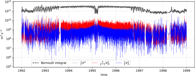
Figure A1. The Bernoulli integral and its terms for the time interval we analyze in this study. The value of the integral (dashed black) is almost identical with the dynamic term (gray), which is the dominant term. The thermal term (red), which assumes adiabatic plasma (γ = 5/3), and the magnetic term (blue) are more than an order of magnitude smaller than the dominant term for the most time.
Download figure:
Standard image High-resolution imageAppendix B: Data Filtering Based on Density Ratios
Within the present paper, we analyze the slow proton population parameters, which normally correspond to the core proton distribution. There are occasions, however, when the magnetic field folds back on itself. On these occasions, the slow population would be the proton beam. In this appendix, we reanalyze the entire time interval, after we exclude all measurements where the density of the slow population is smaller than the density of the fast population. Although this filter enhances the chance that our analysis excludes proton beams, it possibly also excludes intervals where the slow population is the core but for various reasons the beam-to-core density ratio is overestimated. However, this is a novel data filter and suitable for the simple sanity check we want to perform here. Figure B1(a) shows the 2D histogram of  versus
  for the filtered data, in the exact same format as in the right panel of Figure 4. The histogram supports the evidence for subadiabatic behavior of the large-timescale variations of the proton plasma. Panels (b) and (c) of Figure B1 show the polytropic index derived from the analysis of the short-timescale variations as a function of the radial distance and the heliographic latitude, respectively. Although the analysis of the filtered data calculates a slightly higher γ than the one derived from the unfiltered data, it still supports the evidence of the subadiabatic behavior with the characteristic trends over Ulysses' orbit.

Figure B1. Results of the filtered data analysis. (a) 2D histogram of  vs.
vs.  for the entire, filtered data set, in the exact same format as in the right panel of Figure 4. (b) The mean polytropic index determined from the analysis of the short-timescale variations as a function of the radial distance and (c) as a function of heliolatidute.
Download figure:
Standard image High-resolution image