


Abstract
Interstellar neutral (ISN) helium atoms penetrating the heliosphere are used to find the flow velocity and temperature of the very local interstellar medium near the heliosphere. Recently, it was found that, in addition to charge exchange collisions, elastic collisions contribute to the filtration of these atoms outside the heliopause. Momentum exchange between colliding particles related to their angular scattering modifies the properties of the primary and secondary ISN helium populations before the atoms enter the heliosphere. Here, we calculate the transport of ISN helium atoms using plasma and neutral flows from a global three-dimensional heliosphere model. We confirm earlier results based on one-dimensional calculations that the primary population is slowed down and heated by the momentum exchange. Moreover, accounting for momentum exchange in charge exchange collisions results in a faster and warmer secondary population. The paper presents how the velocity and density of these populations vary over the entrance position to the heliosphere. We point out that Maxwell distributions cannot correctly describe these populations. Finally, we calculate the expected Interstellar Boundary Explorer (IBEX) count rates and show that the filtration processes change them significantly. Consequently, future studies of IBEX or Interstellar Mapping and Acceleration Probe (IMAP) observations of ISN atoms should account for these processes.
Export citation and abstract BibTeX RIS

Original content from this work may be used under the terms of the Creative Commons Attribution 4.0 licence. Any further distribution of this work must maintain attribution to the author(s) and the title of the work, journal citation and DOI.
1. Introduction
The heliosphere, created by the solar wind expanding from the solar corona, shields the solar system from most charged interstellar particles (Parker 1961; Zank 1999). Interstellar neutral (ISN) atoms penetrate the heliosphere and allow for direct sampling of interstellar material inside the heliosphere (Blum & Fahr 1970; Wallis 1975a). ISN hydrogen atoms, the most abundant species in the very local interstellar medium (VLISM), are strongly ionized in the heliosphere through charge exchange, photoionization, and electron impact ionization (Bzowski 2008; Bzowski et al. 2013a, 2013b; Sokół et al. 2019a). These processes deplete ISN hydrogen near the Sun (Sokół et al. 2019b). Consequently, the most abundant neutral species at 1 au is the ISN helium (Ripken & Fahr 1983; Fahr & Ruciński 2001). ISN helium atoms are therefore frequently used to infer the VLISM conditions ahead of the heliosphere (Möbius et al. 2004).
The first experiment dedicated to direct sampling of ISN helium atoms was the Ulysses GAS experiment (Witte et al. 1992). The observations from this instrument allowed for derivation of the flow and temperature of ISN helium atoms in the heliosphere (Witte et al. 1996, 2004; Witte 2004; Bzowski et al. 2014; Wood et al. 2015). Launched in 2008, the Interstellar Boundary Explorer (IBEX) is dedicated to observations of neutrals atoms in a broad range of energy (McComas et al. 2009). The low-energy instrument IBEX-Lo (Fuselier et al. 2009) observes ISN atoms of hydrogen, helium, oxygen, and neon (Möbius et al. 2009). Still, the ISN helium flux is dominant, and was used to derive the VLISM parameters in a series of papers (Bzowski et al. 2012, 2015; Möbius et al. 2012; Leonard et al. 2015; Schwadron et al. 2015, 2022; Swaczyna et al. 2018, 2022a; Wood et al. 2019).
The primary ISN atoms originate from the pristine VLISM before the interstellar plasma is substantially affected by the heliosphere presence. In the outer heliosheath, where the interstellar plasma deflects to flow past the heliopause, charge exchange collisions between ISN atoms and ions create the secondary population (Baranov & Malama 1993). The secondary ISN helium population, also known as the Warm Breeze, was discovered in IBEX observations (Kubiak et al. 2014, 2016; Bzowski et al. 2017, 2019). This population was also confirmed in Ulysses GAS data (Wood et al. 2017). The secondary population is warmer and slower because it is created from heated and slowed-down plasma in the outer heliosheath (Kubiak et al. 2014). Moreover, it is also deflected from the primary flow along the so-called neutral deflection plane (Lallement et al. 2005; Kubiak et al. 2016), defined by the pristine VLISM flow and interstellar magnetic field, and thus also called the B–V plane. The deflection of the secondary population informs about the deformation of the heliosphere by the draping magnetic field.
The studies of the ISN helium account for the solar gravitational attraction and ionization processes inside the heliosphere (Lee et al. 2012, 2015; Sokół et al. 2015b). However, most neglect momentum exchange related to angular scattering in elastic and charge exchange collisions. Bzowski et al. (2017, 2019) calculated changes to the velocity distribution function along the trajectories of ISN helium atoms due to charge exchange collisions. However, the momentum exchange in these collisions was neglected. The method of statistical weights was utilized in their papers to calculate the first-order correction to the distribution function based on assumed background distributions from a global heliosphere model (Heerikhuisen et al. 2014; Zirnstein et al. 2016). The statistical weights change along the Kepler trajectory based on gain and loss terms evaluated using the distribution functions from the model. This methodology allows for calculation assuming that the probability of gain and loss is small enough that the multiple collisions of the same atom may be neglected. The charge exchange collisions of helium atoms have been recently included in global modeling by Fraternale et al. (2021) but also without including the related momentum exchange. Inclusion of the elastic and charge exchange collisions with the related angular scattering in the interpretation of the space observations is critical to separate these effects from actual nonthermal signatures in the pristine VLISM (Sokół et al. 2015a; Swaczyna et al. 2019a, 2022b; Wood et al. 2019).
Charge exchange collisions between helium atoms and He+ ions dominate over other charge-changing processes for ISN helium atoms in the outer heliosheath. However, elastic collisions between helium atoms and different interstellar species have comparable cross sections for the typical collision energies in the outer heliosheath. Consequences of these collisions were estimated in several studies in the 1970s and 1980s (Wallis 1975b; Holzer 1977; Fahr 1978; Kunc et al. 1983; Fahr et al. 1985; Chassefière et al. 1986; Gruntman 1986; Chassefière & Bertaux 1987). These analyses considered the collisions using various approximations, including continuous momentum exchange or effective momentum transfer cross sections. These approaches are not appropriate for finding the evolution of the distribution function in the outer heliosheath.
Swaczyna et al. (2021, hereafter Paper I) proposed to use Monte Carlo integration to find the modulation of the distribution function in the outer heliosheath. Their analysis used a one-dimensional cut of a global heliosphere model along the inflow direction (Zirnstein et al. 2016). Paper I demonstrated that elastic collisions in the outer heliosheath are more important than the collisions inside the supersonic solar wind (Gruntman 1986, 2013, 2018) and that they lead to significant heating and slowdown of the primary population.
In this paper, we expand the previous methodology to calculate the changes using the full three-dimensional flows in the outer heliosheath. Moreover, we include charge exchange collisions with related momentum exchange, which were not included in the analysis presented in Paper I. We consider how the primary and secondary population density and velocity depend on the entry position to the heliosphere. Later, the distribution functions obtained from the Monte Carlo integration are presented. Finally, we discuss how momentum exchange in those collisions modifies the ISN helium fluxes observed by IBEX-Lo.
2. Method
The methodology employed here combines two earlier developed methodologies with some modifications. The first task is to calculate the transport of ISN helium atoms from the pristine VLISM to the heliopause, for which we use the methodology presented in Paper I. This part aims to find the distribution functions of primary and secondary helium atoms at a sphere located 100 au from the Sun. To model transport from 100 au to IBEX, we use the analytical full integration model (aFINM; Schwadron et al. 2015). The distance of 100 au is chosen so that it is possibly large but still entirely within the heliosphere. Because we calculate the consequences of the angular scattering outside the heliopause, the transport between 100 au and IBEX does not include further collisions except for ionization losses.
This combination of transport methods is needed to achieve sufficient accuracy of Monte Carlo integration of stochastic collisions outside the heliopause. Because interstellar atoms are tracked along their trajectories from the pristine VLISM, only some of them get inside a sphere of a given radius. In Section 2.1, we briefly describe the global model that we use for our calculations. Details of changes made to the transport model beyond 100 au are discussed in Section 2.2, and further transport with binary collisions is described in Section 2.3.
2.1. Global Model of the Heliosphere
For our analysis, we use results from a global hybrid heliosphere model (Zirnstein et al. 2016; Heerikhuisen et al. 2019). This model uses magnetohydrodynamic equations to solve the plasma flow, while the transport of neutral hydrogen atoms is solved kinetically. The model does not include helium atoms, but instead employs an ad hoc approach to mimic the presence of singly charged helium ions in the VLISM and α particles in the solar wind. The simulation assumes that, during the charge exchange process, the interstellar medium gas He+/H+ ratio is 0.104, such that the effective proton density is 0.05 cm−3 while the total plasma density is 0.0856 cm−3 (see Section 2.3.3 in Zirnstein et al. 2021). The solar wind boundary conditions at 1 au from the Sun are selected to represent the average solar wind conditions over several solar cycles corresponding to the time needed for the ISN helium atom to travel through the heliosphere (Bzowski & Kubiak 2020). The solar wind density is assumed to be 8.3 nuc cm−3 at 1 au and includes 4% of α particles. This density is the mean density from the OMNI data set over four solar cycles before the maximum of solar cycle 24. The velocity and temperature at 1 au are assumed to be 441.5 km s−1 and 51,000 K, respectively. The radial component of the magnetic field assumed to follow the Parker spiral is 37.5 μG at 1 au.
The velocity and temperature at the outer boundary are adopted after McComas et al. (2015). The VLISM inflow speed, inflow direction, and temperature are 25.4 km s−1, (255 7, 51) in ecliptic coordinates, and 7500 K, respectively. The magnetic field strength and direction are 2.93 μG and (22728, 3462), as found by Zirnstein et al. (2016) from the IBEX ribbon position. The effective plasma and neutral hydrogen densities are 0.0856 nuc cm−3 and 0.11 cm−3, respectively. The neutral density is adopted following Bzowski & Heerikhuisen (2020), who showed lower filtration of ISN hydrogen when using appropriate charge exchange cross sections for low collision speeds, typical for the outer heliosheath. This value was estimated for the consensus value of 0.09 cm−3 at the termination shock (Bzowski et al. 2009). The higher ISN hydrogen density estimated from the SWAP observations on New Horizons (Swaczyna et al. 2020) will be considered in the future.
The model provides the density, velocity, and temperature of the plasma and both populations of ISN hydrogen. In the paper, we separate collisions with protons and He+ ions. We assume that both plasma components flow together and have the same temperature. The two populations thermalize in the outer heliosheath due to the Coulomb collisions (Fraternale et al. 2021). We also assume that the density ratio between the proton and He+ is constant in the outer heliosheath with the same proportion as described above. Figure 1 shows the density, radial speed, and temperature of the components along the inflow direction.

Figure 1. Properties of the ISN hydrogen populations and plasma components deduced from the model along the inflow direction. Panels from top to bottom show density, radial speed, and temperature. The secondary ISN hydrogen is produced only within ∼450 au from the Sun; therefore, the presented radial speed and temperature of this population beyond this distance are not physical.
Download figure:
Standard image High-resolution imageThe model results for this study have been discretized on a grid in a Cartesian coordinate system in which the inflow direction coincides with the x-axis, the pristine interstellar magnetic field direction is within the xy-plane, and the z-axis completes the right-handed coordinate system. We use this coordinate system further in the analysis.
2.2. Boundaries of Integration and Initial Conditions
For our study, we focus on obtaining an estimate of the ISN helium distribution function at a spherical surface at dinner = 100 au from the Sun (inner boundary). We extended the Monte Carlo integration scheme described in Paper I to achieve that goal. For each tracked atom, we randomly select a position on the ram half-sphere located at a distance douter from the Sun (outer boundary). We limit considered start positions to the ram half-sphere because the bulk speed of ISN helium atoms exceeds five times their thermal speed (Bzowski et al. 2015). Consequently, it is unlikely for a helium atom at the anti-ram hemisphere to reach the inner boundary. Simultaneously, a random velocity is taken from the assumed pristine Maxwell–Boltzmann distribution of ISN helium far from the heliosphere. The position of an atom and its velocity at infinity defines a Kepler orbit, which we use to find the velocity at the outer boundary (see Appendix A). Therefore, the initial conditions represent atoms on ballistic trajectories originating at infinity, neglecting any possible collisions. While this assumption is not strictly fulfilled, because we expect a comparable number of binary collisions per distance traveled closer to the Sun (Paper I), these collisions should not significantly change the distribution function of interstellar helium, due to the approximate equilibrium between plasma and neutrals far from the heliosphere.
The distance douter ideally should be as large as possible. However, the computational cost of the Monte Carlo integration that provides the same statistics of atoms at the inner boundary changes approximately proportionally to  , because (1) the number of collisions increases proportionally to the traveled distance and (2) the number of particles at the outer boundary is proportional to the surface area of this boundary, i.e., to
  . Therefore, we select douter = 500 au because it provides a reasonable balance between computational costs and at the same time covers the region outside the heliopause that is most affected by the heliosphere. Still, in our initial test sample of 3 × 10⁶ trajectories at the outer boundary, only ∼5.9 × 10⁴ atoms (∼2%) cross the inner boundary.
We need a high statistic of these atoms at this inner boundary to estimate their distribution function. Therefore, we check the minimum distance from the inflow axis for each considered initial position and velocity to limit the number of calculated trajectories that never reach the inner boundary. Figure 2 shows the histogram of this minimal distance from the flow axis for the test sample, separating the primary and secondary populations. Without collisions, only trajectories for which this minimal distance is smaller than 100 au can reach the inner boundary. With elastic collisions, the range of trajectories that can contribute extends to larger values, but the number of contributing trajectories drops by more than 3 decades between 100 and 300 au. The distribution for the secondary atoms is much broader. Still, this distribution also drops significantly around 300 au. Therefore, our further calculations are limited to trajectories for which this minimal distance is smaller than 300 au. As shown in Figure 2, we estimate that this selection leaves out ∼0.004% of primary atom trajectories and ∼0.6% of secondary atom trajectories. However, this selection excludes about ∼75% of initial trajectories, allowing us to speed up our calculations by a factor of ∼4.

Figure 2. Histograms of minimal distances from the flow axis based on initial trajectories of atoms drawn randomly at 500 au that entered the inner boundary. Without collisions, only atoms on trajectories with minimal distances smaller than 100 au enter the inner boundary. The separate histograms are shown for primary and secondary atoms.
Download figure:
Standard image High-resolution imageThe above scheme provides reasonable statistics of ISN atoms that eventually cross the inner boundary. Our full integrations start with 3 × 10⁸ ISN atom trajectories at 500 au, out of which about 7.5 × 10⁷ trajectories pass through the selection of the minimal distance, and about 5.8 × 10⁶ enter the inner boundary.
2.3. Integration of ISN Atom Trajectories with Collisions
The trajectories of randomly drawn ISN helium atoms are integrated following the scheme developed in Paper I with small changes described in this section. Along each trajectory, the properties of four components—namely protons, He+ ions, and two ISN hydrogen populations—are taken directly from the global model (Section 2.1). For each population denoted with subscript k, we calculate the mean relative speed vrel,k using the velocity of the tracked helium atom and assuming that the population k follows a Maxwell–Boltzmann distribution (Ripken & Fahr 1983). The relative speed is further used to calculate the reaction rate using the following formula:

where nk denotes the local density of population k, and σk (vrel,k ) is the total (integral) elastic collision cross section. In this study, we use the cross sections from Paper I. Furthermore, we consider charge transfer collisions between helium atoms and He+ ions. The charge transfer collisions were not included in Paper I, but they are an important part of the ISN helium filtration in the heliosphere (Bzowski et al. 2017, 2019; Fraternale et al. 2021). The charge transfer collisions can be included using the same procedure used for the elastic collisions between helium atoms and ions. The integral cross section for charge transfer is numerically integrated from the differential cross sections calculated in Swaczyna et al. (2021). Figure 3 compares the obtained cross section with the cross section from Barnett (1990).
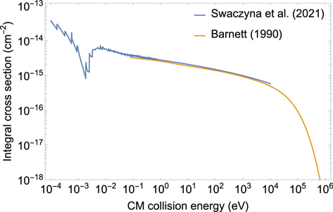
Figure 3. Charge transfer cross section for collisions of He+ ions with helium atoms integrated from differential cross sections calculated by Swaczyna et al. (2021) compared with the cross section from Barnett (1990).
Download figure:
Standard image High-resolution imageAfter the reaction rates are calculated, the trajectory calculation step is

where vatom is the tracked atom speed. This formula chose the calculation step so that it is smaller than 3 au and so that the summed probability of all considered elastic and charge transfer collisions as the atom moves over this distance is smaller than 5%. In Paper I, a constant step of 3 au was used, but in this study, we add the other requirement to reduce the probability that over the distance Δd, the tracked atom may be scattered more than once. Such a situation occurs mainly if the tracked atom speed is very low, e.g., if the neutral atom was created from a slow ion close to the heliopause through a charge exchange collision.
For each calculation step, we evaluate the probabilities of the considered collisions as pk = rk Δd/vatom, and we randomly choose if one of these collisions occurs or if the atom does not collide in this step. For collisions, the scattering angle is selected based on the differential cross sections from Paper I, and the tracked atom velocity is changed accordingly. In case of charge exchange collision, the atom is replaced with a new atom based on the velocity of the parent He+ ion, modified according to the differential charge exchange cross section. Because the charge exchange between He+ ions and helium atoms is the main reaction responsible for losses of the primary ISN helium and gains of the secondary ISN helium, the number of tracked atoms does not change.
After finding the new velocity, the atom position is propagated to the next position based on the atom's velocity. Finally, in each step, the atom velocity is modified to account for the solar gravity  , where α is the solar gravitational parameter (see Appendix A), and
r
is the atom position in the solar reference frame. The atom trajectory is tracked until the atom position is within the forward half-space, i.e., until the x-component of the position is negative (see Section 2.1). We save the atom's state vector (i.e., the velocity and position) where the trajectory crosses the inner boundary at 100 au. However, we continue to track the atoms until they leave the forward half-space, in case the atom trajectory intersects the inner boundary again.
, where α is the solar gravitational parameter (see Appendix A), and
r
is the atom position in the solar reference frame. The atom trajectory is tracked until the atom position is within the forward half-space, i.e., until the x-component of the position is negative (see Section 2.1). We save the atom's state vector (i.e., the velocity and position) where the trajectory crosses the inner boundary at 100 au. However, we continue to track the atoms until they leave the forward half-space, in case the atom trajectory intersects the inner boundary again.
The second intersection is possible in two situations. First, if the perihelion is relatively close to 100 au, the atom after the perihelion may leave this sphere within the forward half-space. While these atoms do not reach IBEX at 1 au, they contribute to the distribution function at 100 au and thus are needed to completely reconstruct the distribution function. The other possible cause of the second intersection occurs is a collision inside the sphere. Because the plasma flow is significantly different, the consequences of this scattering are stronger, especially in cases of charge exchange collisions. Consequently, the atoms scattered inside the inner boundary and escape have significantly changed speeds. These atoms have distinctive velocities compared to the core part, and because they move away from the Sun, we remove them from further analysis.
In our study, we eliminate the state vectors with the velocity components in the Cartesian coordinate system defined in Section 2.1 for which vx ∉ [0, 50] km s−1, vy ∉ [−25, 25] km s−1, or vz ∉ [−25, 25] km s−1. Out of 5.8 × 10⁶ state vectors at the inner boundary, only 22,262 state vectors are removed based on this criterion. Of these, most (21,472) represent atoms moving away from the inner boundary, due to the strong but rare scattering described above. The rest (790) of the removed state vectors represent atoms entering the sphere but with the velocities outside of the adopted range. These state vectors are scattered in the state space, and we cannot find a reasonable probability distribution of these state vectors that could be used to simulate the IBEX signal. Fortunately, because they are far from the core distribution, they are not likely to be interpreted as the ISN helium signal in the IBEX observations.
To separate changes to the primary and secondary populations of ISN He resulting from the angular scattering in collisions from those due to charge exchange only, we repeat the calculation while neglecting momentum exchange in all collisions. This case is calculated with the same number of tracked trajectories as the one with the angular scattering, and a similar number of state vectors cross the boundary at 100 au. Furthermore, we also verified our tools with two additional tests. In the first test, we check whether the distribution at 100 au is the same as that at 500 au in the absence of the gravitational forces, elastic, and charge exchange collisions. In the other test, we include gravity, finding that the change to the bulk speed is the same as predicted for cold atoms.
3. Density of the ISN Helium at 100 au
The primary and secondary populations of the ISN helium are likely to have significantly different properties. Therefore, we separate these populations depending on whether the given trajectory was modified by charge exchange collision somewhere between 500 and 100 au. Beyond 500 au from the Sun, the properties of the plasma and neutrals do not differ from each other, and the charge exchange collisions do not change the statistical properties of these populations. Nevertheless, the selection of this distance within 500 au significantly modifies the secondary population properties (see Section 7.1).
To derive the properties of the ISN helium populations at 100 au, we assign weights to the state vectors based on the flux through the boundary at 500 and 100 au. We draw initial state vectors at the outer boundary using the distribution functions as the probability distribution. The flux of the particles through the outer and inner boundaries is proportional to the distribution function multiplied by the atoms' radial speed. Because both boundaries are spherical, the flux is given by the distribution function times the local radial velocity. Therefore, to find the properties of the distribution function at the inner boundary, the weights are given by the ratio of the radial speed at 500 au to the radial speed at 100 au:

where v outer and v inner are the tracked atom velocities at the outer (router = 500 au) and inner (rinner = 100 au) boundaries, respectively, while r outer and r inner are corresponding positions.
With the above weighting, we analyze the distribution function starting with the density of the atoms crossing the boundary as a function of the position on this boundary. We split the forward hemisphere based on the projection of points from the hemisphere at 100 au to the plane perpendicular to the flow direction. As defined in Section 2.1, we use coordinates y and z in this plane. Note that the interstellar magnetic field far from the heliosphere is within the xy-plane. Moreover, the x-coordinate of the inner hemisphere can be calculated as  . In this plane, we split the surface into cells [yi
± Δy, zi
± Δz], where Δy = Δz = 10 au, i = 0, 1,...,20 and j = 0, 1,...,20 enumerate the cells centered at yi
= − 90 + i × 20 au, zj
= − 90 + j × 20 au. Twelve of these cells in the corners of the yz-plane are outside of the projection of the hemisphere. Moreover, some cells are only partially within this projection. For each cell that is at least partially within the projection, we calculate the surface area of the sphere projecting onto each cell.
. In this plane, we split the surface into cells [yi
± Δy, zi
± Δz], where Δy = Δz = 10 au, i = 0, 1,...,20 and j = 0, 1,...,20 enumerate the cells centered at yi
= − 90 + i × 20 au, zj
= − 90 + j × 20 au. Twelve of these cells in the corners of the yz-plane are outside of the projection of the hemisphere. Moreover, some cells are only partially within this projection. For each cell that is at least partially within the projection, we calculate the surface area of the sphere projecting onto each cell.
The density of each population in a given cell is proportional to the sum of the weights (Equation (3)) of the final state vectors at the inner boundary with the position in the yz-plane within this cell, normalized by the surface area of the cell Ωij , and the total number of initial state vectors drawn in the Monte Carlo integration Ninit:

The proportionality factor C = 1.563821 × 10⁶ au2 is selected so that, in the test case without collisions and gravitational attraction, the density is 1 on the entire inner boundary. Therefore, the densities presented here show a density relative to the ISN helium density far from the Sun.
The densities of both populations obtained from the Monte Carlo results are presented in the top row of Figure 4. The density of the primary population does not depend significantly on the position on the inner boundary, and it is between 0.89 and 0.925 of the density far from the Sun. However, the secondary population density is noticeably higher closer to the inflow direction ( au), ∼0.085 compared to ∼0.07 far from this direction (
 au). This figure also shows the results for the case without angular scattering, which are in this respect very similar. The middle row presents polynomial fits to the numerical result (Appendix B), to emphasize the main differences in the properties.

Figure 4. Estimated density of ISN helium populations normalized to the ISN helium density in the pristine VLISM as a function position at 100 au from the Sun. The inflow direction (v∞) and the magnetic field (B∞) direction in the pristine VLISM projected onto the inner boundary are marked. The two left (right) columns show results for the primary (secondary) ISN helium. The first and third (second and fourth) columns show the result from calculations with (without) angular scattering. All presented results account for charge exchange collisions. The top row shows the result of Monte Carlo integration, the middle row shows the results of the polynomial model (Appendix B), and the bottom row shows the residuals.
Download figure:
Standard image High-resolution image4. Bulk Velocity of the ISN Helium at 100 au
The bulk velocities of the ISN helium populations are calculated on the same grid at 100 au from the Sun as for the density calculations in Section 3. The velocity components in the xyz-coordinates are calculated from the results of Monte Carlo integration as averages of the velocity components of the trajectories ending at 100 au in each cell using weights given in Equation (3). The obtained bulk velocities of the primary and secondary ISN helium components are presented in the top rows of Figures 5 and 6, respectively. The middle rows show the analytic model (Appendix B).

Figure 5. Bulk velocity of the primary ISN helium distribution. The left (right) three columns show the results from calculations with (without) angular scattering. Within the respective groups, consecutive columns show the x, y, and z components. The top row shows the result of Monte Carlo integration, the middle row shows the results of the polynomial model (Appendix B), and the bottom row shows the residuals.
Download figure:
Standard image High-resolution image
Figure 6. The same as Figure 5, but for the secondary population.
Download figure:
Standard image High-resolution imageSeveral factors change the velocity of the ISN helium atoms before they enter the heliosphere. Even in the absence of collisions, the population bulk velocity changes due to attraction in the solar gravitational field. The change in the velocity of the primary population due to charge exchange collisions is very small and is related to the preferential removal of atoms from some portion of the distribution function (Bzowski et al. 2019). In the proximity of the flow direction, the speed remains effectively unchanged Δvpri = (0.015, 0.004, 0) km s−1 compared to the flow speed modified just by gravitational attraction (see Appendix B). With the angular scattering, the velocity changes much more significantly by Δvpri = (–0.6, –0.11, 0) km s−1. The change in the x-component is consistent with the change obtained from the one-dimensional analysis in Paper I. We also find a statistically significant deflection in the y-direction. This effect results from collisions with plasma diverted along the heliopause flowing radially outward in the frontal part of the heliosphere.
The secondary component is also affected by momentum exchange. Without angular scattering, the bulk velocity along the flow direction is  = (12.9, –2.3, 0) km s−1, and with angular scattering, it is
  = (13.9, –2.2, 0) km s−1. Therefore, in contrast to the change in the primary population, which is slowed down, the secondary population is faster by ∼1 km s−1 relative to the Sun if the angular scattering is included. Because angular scattering causes some momentum exchange in charge exchange collisions, the secondary population gains momentum from the primary population, which is faster than the plasma.
5. Distribution Function of ISN Helium at 100 au
In this section, we aim to describe the distribution functions of these populations. We seek common distribution functions describing these populations at 100 au to describe the higher moments of the distribution function, which require higher statistics of Monte Carlo integrated trajectories. Due to the asymmetry of these distributions (Swaczyna et al. 2019b; Paper I), we need to rotate the obtained state vector to a coordinate system where the local bulk flow defines one of the axes. Consequently, in the first step, we rotate the obtained velocities at 100 au,
v
, according to the local bulk flow velocity of the respective population,  , obtained from the analytic formulae (Appendix B) at the point at which the atom entered the inner boundary:

where R [ u , w ] is a rotation matrix rotating vector u to be aligned with the direction given by vector w about an axis defined by the cross product of these two vectors. In the rotated coordinate system, we define parallel and two perpendicular components: v rot = (v∥, v⊥1, v⊥2). The two perpendicular components are not equivalent, because the B–V plane introduces an asymmetry in the y-direction. Consequently, we consider these two directions separately. For each velocity component, we calculate one-dimensional histograms with weights calculated from Equation (3).
The obtained histograms for the primary populations are presented in Figure 7. We use asymmetric one-dimensional kappa distribution, as defined in Paper I, to model the distribution functions of the primary population's parallel and first perpendicular components. This distribution is characterized by two temperatures (T) and kappa indices (κ), separate for the speeds below (denoted with subscript "1") and above (subscript "2") the speed (u) in the rotated frame. For example, in the parallel component, the subscript "1" corresponds to the part slower relative to the Sun, while the subscript "2" denotes the faster part. The second perpendicular component is defined using the symmetric one-dimensional kappa distribution. The obtained parameters of this distribution are shown in Table 1 and are compared with the result of one-dimensional calculations from Paper I. For large values of the κ parameter, the distribution is not distinguishable from Maxwell within the range available here. Therefore, for κ > 1000, we report this value as ∞, which means that the limit κ → ∞ may be applied.
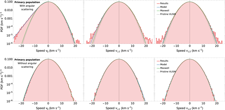
Figure 7. Histograms and modeled distribution functions of the primary ISN helium population in the rotated coordinate system. The components v∥, v⊥1, and v⊥2 are shown in columns from left to right. The histograms obtained from Monte Carlo integration are shown as red areas. The analytic model functions selected for each component are shown as blue lines, and the Maxwell fit with green lines. The distribution function in the pristine VLISM is shown with dashed gray lines. The top and bottom rows show the results with and without angular scattering, respectively.
Download figure:
Standard image High-resolution imageTable 1. Parameters of the Primary ISN Helium Distribution at 100 au
| Component | Calculation | Ang. Scatt. | u | T1 | κ1 | T2 | κ2 |
|---|---|---|---|---|---|---|---|
| (km s−1) | (K) | (1) | (K) | (1) | |||
| v∥ | 3D | W/o | −0.07 | 7110 | ∞ | 7440 | ∞ |
| v∥ | 3D | With | 0.28 | 9980 | 7.5 | 7790 | ∞ |
| v∥ | 1D (Paper I) | With | 0.25 | 10600 | 6.5 | 7950 | ∞ |
| v⊥1 | 3D | W/o | 0 | 7550 | ∞ | 7580 | 110 |
| v⊥1 | 3D | With | 0 | 8350 | 37 | 8230 | ∞ |
| v⊥2 | 3D | W/o | ≡0 | 7550 | ∞ | ≡T1 | ≡κ1 |
| v⊥2 | 3D | With | ≡0 | 8230 | 130 | ≡T1 | ≡κ1 |
| v⊥ | 1D (Paper I) | With | ≡0 | 8650 | 30 | ≡T1 | ≡κ1 |
Download table as: ASCIITypeset image
The primary population is significantly heated in our current calculations—but it is less heated, by a few hundred kelvins, than predicted in Paper I. The main reason for this discrepancy is that, in the one-dimensional calculations, we use the plasma parameters along the flow direction, where plasma is more significantly heated than, on average, away from the flow direction where some of the ISN helium atoms originate from in this analysis. Additionally, we find a Maxwellian fit to the calculated distribution limited to the part of the histogram above 10% of the maximum value. This fit provides approximate Maxwellian parameters of the distribution close to the peak. The fit distributions are centered at +0.13 km s−1 and –0.01 km s−1 relative to the bulk speed for the respective cases with and without the scattering, and the temperatures are 8180 K and 7380 K, respectively. The apparent cooling of the primary ISN helium population in the parallel component is related to the change in the gravitational field of the Sun. Moreover, this effect introduces a small asymmetry of the distribution function.
The obtained histograms for the secondary population are shown in Figure 8. For this population, the parallel component cannot be effectively modeled using the asymmetric kappa distribution. Consequently, we use a sum of four Maxwell distributions to model this highly asymmetric distribution in the parallel component. We fit four components characterized by the speed (u) relative to the bulk flow speed, temperature (T), and weight factor (ξ). The weights for all four components sum to unity because each component is normalized. For the perpendicular components, we use the same distribution functions as for the primary population. The parameters of these distributions are shown in Table 2. The steep cutoff on the left side of the parallel velocity distribution corresponds to atoms at rest relative to the Sun. Therefore, the lack of atoms on the left of this cutoff is because it would show particles created inside the inner boundary at 100 au from the Sun.
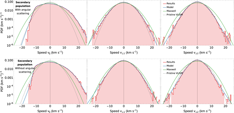
Figure 8. As in Figure 7, but for the secondary ISN helium population.
Download figure:
Standard image High-resolution imageTable 2. Parameters of the Secondary ISN Helium Distribution at 100 au
| Component | Ang. Scatt. | ξ | u | T1 | κ1 | T2 | κ2 |
|---|---|---|---|---|---|---|---|
| (1) | (km s−1) | (K) | (1) | (K) | (1) | ||
| v∥ (1) | W/o | 0.045 | −9.75 | 690 | ⋯ | ⋯ | ⋯ |
| v∥ (2) | W/o | 0.178 | −6.07 | 2580 | ⋯ | ⋯ | ⋯ |
| v∥ (3) | W/o | 0.405 | −0.71 | 6880 | ⋯ | ⋯ | ⋯ |
| v∥ (4) | W/o | 0.372 | 4.79 | 13600 | ⋯ | ⋯ | ⋯ |
| v∥ (1) | With | 0.035 | −9.73 | 760 | ⋯ | ⋯ | ⋯ |
| v∥ (2) | With | 0.127 | −6.77 | 3160 | ⋯ | ⋯ | ⋯ |
| v∥ (3) | With | 0.412 | −1.94 | 7560 | ⋯ | ⋯ | ⋯ |
| v∥ (4) | With | 0.426 | 4.62 | 13250 | ⋯ | ⋯ | ⋯ |
| v⊥1 | W/o | ≡1 | −0.30 | 8800 | 10.0 | 10040 | 16.7 |
| v⊥1 | With | ≡1 | −0.15 | 10310 | 15.8 | 10920 | 45 |
| v⊥2 | W/o | ≡1 | ≡0 | 7220 | 8.8 | ≡T1 | ≡κ1 |
| v⊥2 | With | ≡1 | ≡0 | 8520 | 12.8 | ≡T1 | ≡κ1 |
Download table as: ASCIITypeset image
As with the primary population, we fit Maxwell distributions to the obtained results, which give temperatures of 13,950 K and 12,620 K with centers shifted by –0.38 km s−1 and –0.41 km s−1 in the parallel direction relative to the bulk speed, respectively, for the calculations with and without angular scattering. Nevertheless, the Maxwell fits show very poor consistency with the results and should not normally be used for analyses. Comparison with the Maxwellian for the temperature of 9500 K, as obtained by Kubiak et al. (2016), shows that, while the temperature is similar to our results in the perpendicular components, it is much too low to describe the parallel component. However, the temperature of the secondary population found here is lower than the estimate of ∼25,500 K obtained by Fraternale et al. (2021) in a self-consistent model accounting for helium atoms and ions, which does not account for the angular scattering. As discussed in Section 7.1, this may be partially caused by the arbitrary separation of the primary and secondary components.
While the provided functions effectively describe the one-dimensional distribution function in the selected directions, the full three-dimensional distribution of each population may not be represented by a simple product of these three components, due to possible correlations. To verify that, we plot cross sections through three-dimensional histograms with the bin size of (1 km s−1)3 in Figures 9 and 10 for the primary and secondary ISN helium population, respectively, calculated with angular scattering. The results are compared with the value obtained from the product of the three component distributions. The differences between these two estimates show systematic patterns due to correlations between components.

Figure 9. Two-dimensional cross sections through the three-dimensional histogram of the primary ISN helium population obtained from the calculations with angular scattering. The columns show three different cross-sectional planes defined by v⊥2 = 0, v⊥1 = 0, and v∥ = 0. The rows from top to bottom show the numerical distribution obtained from Monte Carlo integration, reconstruction from the analytic model given by the product of three components, the difference between the above two, the nonanalytic additive (see text), and the final residuals.
Download figure:
Standard image High-resolution image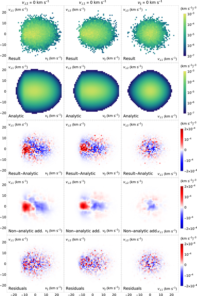
Figure 10. As in Figure 9, but for the secondary ISN helium population.
Download figure:
Standard image High-resolution imageTo account for these correlations between components, we perform a Gaussian smoothing with a three-dimensional Gaussian distribution with width σ = 2 km s−1 in each dimension. This smoothing is performed over the entire three-dimensional distribution, and the results for the chosen cross sections are presented in Figures 9 and 10. The results of the smoothing are hereafter called nonanalytic additives. These additives show correlated structures, especially between the parallel component and each of the perpendicular components, which cannot be represented by analytical distribution given as a product of three one-dimensional distributions. For example, the secondary population is narrower in the perpendicular direction for the most negative parallel speeds in the secondary population flow frame than the particles with positive parallel speeds. Consequently, the populations at 100 au can only be approximated using the analytic product of the distribution functions in each direction. The residuals additionally accounting for the nonanalytic additives are also presented in these figures.
6. Consequences for ISN Helium Observations with IBEX-Lo
We use the analytical full integration model (aFINM; Schwadron et al. 2013, 2015, 2016; Rahmanifard et al. 2019) to calculate the IBEX flux based on the distribution functions. The model is updated to track atom trajectories only to 100 au from the Sun using the procedure provided in Appendix A. Moreover, it is modified to use position-dependent numerical distributions obtained in this study rather than assuming a homogeneous Maxwell distribution at infinity. The distribution functions are discretized using the same grid in space and velocity as in Sections 3–5.
The expected flux at IBEX is integrated over the IBEX angular response and spin angle bins, and averaged over the observation time. However, the energy response function is assumed constant, and the model integrates over the expected ISN helium atom energy range. The integrated fluxes are scaled by a constant factor to match the maximum flux observed by IBEX-Lo on orbit 16 in ESA 2. This energy step is the most suitable reference because the energy response is expected to be approximately constant over the relevant energy range (Schwadron et al. 2022). The orbit/orbital arc selection includes observations made with the IBEX spin axis pointing longitude between 235° and 335°, which corresponds approximately to the IBEX ecliptic longitude from 55° to 155°. This selection includes the secondary ISN helium signal but avoids data with significant contribution from the ISN hydrogen atoms (Swaczyna et al. 2018). The obtained fluxes are projected onto a skymap using the same procedure as in Swaczyna et al. (2018, 2022a).
To find the significance of the angular scattering and the details of the ISN helium distribution function for the IBEX observations, we calculate the expected flux for the distribution functions for the cases with and without the scattering. Figure 11 presents the results obtained using the combined distribution function of the primary and secondary ISN helium populations reconstructed from the analytic formulae with the nonanalytical additive, obtained from smoothing the original residuals (see Section 5), included (we refer to this as a "full" model). Due to the large dynamical range of the observed fluxes, the top two panels showing the results for the two cases are almost identical. However, the difference in the bottom panel reveals how the signal changes due to the angular scattering. The peak count rate decreases by ∼2 s−1, i.e., about 10% of the peak count rate. Around the peak, the signal is enhanced but somewhat asymmetric, as it is increased on the side where the secondary population is more prominent (right from the peak). Moreover, the peak reduction is shifted to the left from the peak. These two changes are because of the slowdown and heating of the primary population. The flux is reduced in the right portion, where the secondary population is most prominent. This effect is caused by the higher speed of the secondary population when the angular scattering is accounted for (see Section 4). The results show that the momentum exchange is important both for the primary population, which is slowed down and heated, as well as for the secondary population, which gains momentum and thus is less gravitationally deflected.

Figure 11. The expected IBEX count rates from the ISN helium limited to the ISN helium-dominated region (marked with white dashed box) for the cases with (top panel) and without (middle panel) angular scattering, as well as their difference (bottom panel). The bottom panel has a two-sided logarithmic color bar, where changes less than ±0.01 s−1 are marked as black. The maps show the orientation of the B–V plane defined by the flow of the primary ISN helium (V; Swaczyna et al. 2022a) and the interstellar magnetic field (B; Zirnstein et al. 2016). The inflow direction of the secondary population is also shown (S; Kubiak et al. 2016).
Download figure:
Standard image High-resolution imageBeyond the change caused by the angular scattering, we also verify how the details of the distribution function are reflected in the modeled IBEX flux. For this purpose, we calculate the case with the angular scattering using three versions of the distribution function. The first uses the binned distribution function obtained directly from Monte Carlo integration, which we later refer to as the "numerical" distribution. The next is the full model, i.e., the distribution modeled using the analytic function and the nonanalytic additive ("full"). Finally, the last distribution function is reconstructed only from the analytic function.
Figure 12 shows the expected difference in the IBEX observations between these three distribution functions. The numerical model does not assume any specific form of the distribution function, but it shows significant numerical variation for individual orbits. The difference between the numerical and analytic models shows some large structures in the sky with a count rate difference between –0.4 and 0.3 s−1. This show that the analytic approximation of the distribution function cannot fully reproduce the complexity of the three-dimensional distribution functions resulting from filtration in the heliosphere boundaries. The difference is significantly reduced with the full model to between –0.16 and 0.09 s−1, i.e., approximately three-fold. These changes are much smaller than the consequences of the angular scattering. Still, some structures are visible, suggesting that the full model may not fully describe the processed distribution functions. Therefore, while the analytic model may be used as the first approximation, including the nonanalytic component may be necessary for future quantitative comparisons with the IBEX data. We also performed the same analysis for the case without the angular scattering, which shows less complex patterns, but the amplitude of differences is similar.
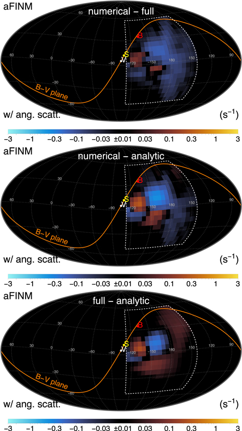
Figure 12. Differences between the expected count rates for the models with the angular scattering. The panels from top to bottom show the differences between the numerical and full models, the numerical and analytic models, and the full and analytic models.
Download figure:
Standard image High-resolution image7. Discussion
This study broadens the analysis in Paper I by including the charge exchange collisions with the related angular scattering in this process. First, we perform the calculation in three-dimensional space. Moreover, we included charge exchange collisions with the related angular scattering. This broadening provides means to discuss the role of the secondary population and its separation from the primary population (Section 7.1). Furthermore, we discuss the consequences of the angular scattering for interpreting the VLISM parameters derived from the IBEX observations (Section 7.2).
7.1. Separation of the Primary and Secondary Populations
Charge exchange collisions create secondary atoms in the part of the VLISM affected by the presence of the heliosphere. Beyond the region of the heliosphere's influence, the charge exchange collisions do not generally impact the distributions of neutrals and ions, as they are typically assumed to remain in thermal equilibrium. However, the parameters of the VLISM derived from IBEX observations suggest that there is no bow shock ahead of the heliosphere (McComas et al. 2012), and thus the region affected by the heliosphere is not well-defined. Due to neutral atoms propagating throughout the VLISM in the model, the range of the heliosphere influence may extend beyond the bow wave. Consequently, also the definition of the secondary population is not very precise. In this study, all atoms that are the result of charge exchange collisions within the computational region up to 500 au from the Sun are called the secondary population. As shown in Section 5, the population of the secondary atoms is not well-described by a single Maxwell distribution because the secondary atoms originate from the VLISM plasma, which is decelerated progressively depending on the distance from the heliopause. While the plasma flow is almost identical to the neutrals at 500 au, the radial plasma flow speed drops to almost zero near the heliopause. Consequently, the distance at which the newly created atoms are classified as the secondary population significantly impacts the secondary population parameters and distribution. We checked that the secondary atoms produced by charge exchange only within 300 au from the Sun have a bulk speed of ∼12 km s−1, compared to ∼15 km s−1 for 500 au. This change also affects the properties of the primary population. Including all secondary atoms created between 300 and 500 au in the primary population changes the primary population bulk speed by about 0.3 km s−1. Fraternale et al. (2021) used a criterion based on the plasma temperature, which extends the production region to ∼550 au, and estimated the secondary population speed at 12.5 km s−1, which is close to the 13.1 km s−1 obtained in our study in the case without the angular scattering.
The distinction between the primary and secondary atoms is conventional. Because the distribution functions of these populations overlap, there is no clear way to separate these two populations. The original interpretation of the IBEX observations using two Maxwell distributions, the first corresponding to the primary population and the other describing the Warm Breeze, is only an approximation. The analysis by Kubiak et al. (2019) and our study show that the secondary population is not a Maxwell distribution but rather is a highly distorted population that can only be calculated by solving a transport equation with gains and losses due to the charge exchange collisions. The apparent consistency of the IBEX observations with the two Maxwell distributions shown by Kubiak et al. (2014, 2016) does not prove that these populations describe the outer heliosheath distribution of the ISN helium. While the two Maxwell model is a convenient way to show consistency with the IBEX data, our results show that it is invalid.
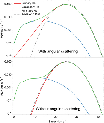
Moreover, while the primary population is faster relative to the Sun, the extended tail formed because of momentum transfer in elastic collisions forms at lower speeds and coincides with the secondary population. Figure 13 compares the distribution function along the parallel component of the primary and secondary population 100 au from the Sun at the inflow direction using the analytical model obtained in this study. The figure shows that the secondary population contribution dominates over the extended tail of the primary population. Consequently, the main difference that may be observed with the primary population is the shift of the peak speed rather than the extended tail, which remains hidden under the secondary population.
Figure 13. Probability distribution function of the primary (red line), secondary (blue), and combined (green) populations of ISN helium at 100 au from the Sun along the inflow direction. The results are compared with the pristine VLISM distribution (dashed gray). The top and bottom panels show the results with and without angular scattering, respectively.
Download figure:
Standard image High-resolution image
7.2. Interpretation of the IBEX-derived VLISM Flow Parameters
The prior analyses of observations of ISN helium atoms neglected the angular scattering of ISN atoms in the heliosphere. Because these analyses were used to find the properties of the VLISM near the heliosphere, our study shows that these results require reinterpretation. Our analysis shows that both populations undergo significant changes. However, due to challenges related to the separation of the primary and secondary populations, we refrain from interpreting the previous parameters of the secondary population. Therefore, we focus on the primary ISN helium population, which is used to find the pristine VLISM properties.
Paper I, which used only a simplified one-dimensional model of the flow outside the heliopause, showed that the ISN helium is slowed down by ∼0.45 km s−1 and heated by ∼1100 K. Our analysis provides that the bulk flow of the primary population decreases by ∼0.61 km s−1 with the inclusion of the angular scattering (Section 4). However, accounting for the shift in the Maxwell distribution peak (Section 5), the actual difference between the mean speed of the Maxwell fit is reduced to 0.47 km s−1. Therefore, our new result is close to the previous estimation. Furthermore, the scattering heats the primary population by ∼800 K, i.e., ∼300 K less than obtained in Paper I. With the most recent parameters obtained from the 12 yr of the ISN helium observations with IBEX (Swaczyna et al. 2022a), the revised velocity of the pristine VLISM is ∼25.9 km s−1 and the temperature is ∼6450 K.
8. Summary and Conclusions
ISN helium atoms are used to derive the VLISM conditions near the heliopause because they are the most abundant species near the Sun. However, most analyses of ISN helium observations have not accounted for filtration of the ISN helium population by charge exchange and elastic collisions. This paper presents comprehensive modeling of these filtration processes, including the appropriate momentum exchange leading to angular scattering of the colliding particles. We solved the transport of the ISN helium accounting for these processes with Monte Carlo integration using a three-dimensional global heliosphere model, including the flows in the VLISM.
We found that these collisions modify both the primary and secondary populations of the ISN helium. We assumed that the atoms created through charge exchange from the He+ ions within 500 au from the Sun are classified as the secondary population. Based on this assumption, the ISN helium population consists of ∼91.5% of primary atoms and ∼8.5% of secondary atoms near the nose direction. The combined density of these populations away from the inflow direction is slightly reduced compared to the pristine VLISM density.
Elastic collisions and charge exchange losses of primary ISN helium atoms result in a slower and warmer population near the heliopause. The slowdown is generally similar to that found earlier (Paper I) using one-dimensional calculations. The increase in the population temperature is smaller compared to the previous estimates. The analysis of the secondary population shows that it is faster and warmer if the angular scattering is included in the calculations. The opposite change of the velocity results from the momentum exchange, which generally slows down the primary population because, on average, these atoms collide with slower populations, while the secondary population speeds up because the secondary atoms gain some momentum in the charge exchange collisions.
Our analysis shows that the Maxwell distribution function cannot correctly describe either population. The primary population is asymmetric, with a tail of slow atoms relative to the Sun resulting from significant momentum exchange in elastic collisions. The secondary population is much more complex than the primary population. The populations can be approximated using analytic formulae for three dimensions relative to the local flow of the populations at 100 au. However, this approach does not fully reproduce the actual three-dimensional velocity distribution function. Consequently, the full description of these populations is possible only using numerical distribution functions.
We calculated the expected fluxes at IBEX and found that the angular scattering significantly changes the expected count rates. The changes are significant, considering the improved statistics of the IBEX observations of ISN helium atoms, which allowed for a significant reduction of the VLISM parameter uncertainties derived from the analyses of these observations. Future analyses of IBEX observations of ISN helium atoms should account for changes due to these collisions in a self-consistent way. We plan to perform a quantitative comparison between the IBEX data and models in a future analysis. This approach will also be necessary to interpret observations from the IMAP-Lo instrument planned on the Interstellar Mapping and Acceleration Probe (IMAP; McComas et al. 2018). IMAP-Lo enables observations with greater flexibility provided by a movable platform (Sokół et al. 2019c; Bzowski et al. 2022; Schwadron et al. 2022).
This material is based upon work supported by the National Aeronautics and Space Administration under grant No. 80NSSC20K0781 issued through the Outer Heliosphere Guest Investigators Program. P.S. thanks Hans-Reinhard Müller for helpful discussion about solving Kepler trajectories.
Appendix A: Kepler Trajectories
We use analytic formulae describing the trajectories of ISN atoms in the heliosphere for two purposes. First, we calculate the change in the bulk speed due to gravitational attraction in the solar gravitational field (Appendix B). Moreover, we use this formulation to track ISN atoms from the inner boundary of the Monte Carlo calculations to IBEX (Section 6). The Kepler orbit of an ISN atom may be defined by the complete state vector (position r 0 and velocity v 0) of an atom at any point along its trajectory—or in the case of an atom on hyperbolic orbits, by the position of the atom r 0 and the velocity at infinity v ∞. This appendix provides a summary of the equations used in our study. For a full derivation, we refer the reader to textbooks (e.g., Smart & Green 1977).
In the first case, we find the specific angular momentum ( h ) and the eccentricity ( e ) vectors calculated as


where α = GM⊙ = 1.3271244 × 10²² m3 s−2 = 887.128 au km2 s−2 is the standard gravitational parameter of the Sun (e.g., Particle Data Group et al. 2020). The eccentricity vector is proportional to the Laplace–Runge–Lenz vector. The orbit is in the plane perpendicular to h , and the orbit eccentricity is given by the modulus of the eccentricity vector e = ∣ e ∣. The orbital parameter is given as

which can be used to find the radial distance as a function of the true anomaly θ:

The perihelion position can be expressed using the eccentricity vector:

We need to find a state vector at a specified distance from the Sun in our problem. The true anomaly corresponding to distance r can be calculated by inverting Equation (A4):

where s is either –1 before the perihelion or +1 after the perihelion. The position at a given distance can be calculated using the Rodrigues rotation formula applied to the normalized eccentricity vector, which points to the perihelion position rotated about the specific angular momentum vector:
The velocity at this position can be calculated from the following formula:
One can verify that Equations (A7) and (A8) lead to the same angular momentum and eccentricity.
If the Kepler trajectory is defined by the position r 0 and velocity at infinity v ∞, derivation of the trajectory requires a few additional steps. Far from the Sun, the trajectory is a straight line parallel to the velocity vector direction shifted from the line crossing the Sun by the impact parameter vector b :

The direction of the impact parameter vector is perpendicular to the velocity far from the Sun and to the vector normal to the plane of the trajectory. The plane is defined by any combination of the position and velocity for a given orbit, including the initial position and the velocity at infinity. Therefore, the normalized impact parameter must be equal to

The impact parameter value can be calculated from the procedure described by Fahr (1968). First, the angle between the velocity at infinity and the initial position is calculated from the following relations:

With this angle, the impact parameter value is
where s is equal to –1 if the position r 0 is before the perihelion or +1 if it is after the perihelion.
With the impact parameter calculated, the specific angular momentum and eccentricity vectors are


Further calculations follow the previous case.
Appendix B: Analytic Functions Describing Density and Velocity of ISN Helium Populations
To find analytic functions describing the densities of each population as a function of the position at the inner boundary of our calculations, we consider a polynomial of the maximum degree equal to 4 in the following form:
where ai,j
are polynomial coefficients. In general, this polynomial consists of 15 monomials. However, our results follow a mirror symmetry with respect to the xy-plane, which is defined by the inflow direction and the interstellar magnetic field far from the Sun. Therefore, we assume that  . This requirement means that coefficients ai,j
for j = 1 or 3 must be 0, which reduces the number of considered coefficients here to 9. We find the best-fitting coefficients using the least-squares method. The obtained coefficients are presented in Table B1. The densities reproduced from this polynomial are also presented in the middle row of Figure 4. Finally, the residuals are shown in the bottom row of this figure. The residuals are randomly scattered, showing that the density can be modeled with the above polynomial. The standard deviation of the residuals for the primary and secondary populations are 0.006 and 0.003, respectively.
. This requirement means that coefficients ai,j
for j = 1 or 3 must be 0, which reduces the number of considered coefficients here to 9. We find the best-fitting coefficients using the least-squares method. The obtained coefficients are presented in Table B1. The densities reproduced from this polynomial are also presented in the middle row of Figure 4. Finally, the residuals are shown in the bottom row of this figure. The residuals are randomly scattered, showing that the density can be modeled with the above polynomial. The standard deviation of the residuals for the primary and secondary populations are 0.006 and 0.003, respectively.
Table B1. Polynomial Coefficients for Densities and Velocities of the ISN Helium Populations
| Population | Quantity(Unit) | Ang. Scatt. | Polynomial Coefficients | ||||||||
|---|---|---|---|---|---|---|---|---|---|---|---|
| a0,0 | a0,2 | a0,4 | a1,0 | a1,2 | a2,0 | a2,2 | a3,0 | a4,0 | |||
| Primary | npri/n∞ (1) | With | 0.9127 | 0.0239 | −0.0255 | 0.0017 | −0.0041 | 0.0263 | −0.0399 | 0.0002 | −0.0300 |
| Primary | npri/n∞ (1) | W/o | 0.9055 | 0.0208 | −0.0276 | 0.0018 | −0.0022 | 0.0207 | 0.0019 | 0.0047 | −0.0240 |
| Secondary | nsec/n∞ (1) | With | 0.0851 | −0.0014 | −0.0189 | −0.0041 | 0.0002 | −0.0089 | −0.0085 | 0.0013 | −0.0099 |
| Secondary | nsec/n∞ (1) | W/o | 0.0861 | −0.0101 | −0.0071 | −0.0042 | −0.0009 | −0.0169 | −0.0068 | 0.0013 | −0.0013 |
| Primary | Δvpri,x (km s−1) | With | −0.6049 | −0.0354 | 0.0679 | 0.0048 | −0.0100 | −0.1209 | 0.2853 | −0.0023 | 0.1714 |
| Primary | Δvpri,x (km s−1) | W/o | 0.0148 | −0.0001 | 0.0056 | −0.0205 | 0.0695 | 0.0299 | −0.0022 | 0.0206 | −0.0206 |
| Secondary |
v
 (km s−1) (km s−1) | With | 13.9366 | 0.7961 | 0.8936 | −0.5741 | 0.6026 | 1.3131 | −0.7195 | 0.6235 | 0.1013 |
| Secondary |
v
 (km s−1) (km s−1) | W/o | 12.9249 | 1.4764 | 0.1453 | −0.2992 | 0.1631 | 2.1871 | −1.3692 | 0.3051 | −0.8095 |
| Primary | Δvpri,y (km s−1) | With | −0.1126 | 0.0372 | −0.0804 | 0.1717 | −0.1213 | −0.0172 | −0.0240 | −0.1595 | 0.0071 |
| Primary | Δvpri,y (km s−1) | W/o | 0.0035 | −0.0767 | 0.0655 | 0.0738 | −0.1184 | −0.0731 | 0.1949 | −0.1748 | 0.0709 |
| Secondary |
v
 (km s−1) (km s−1) | With | −2.1815 | 0.2644 | 0.0886 | 1.0861 | −0.5650 | 0.8052 | −0.5009 | −0.7738 | −0.5139 |
| Secondary |
v
 (km s−1) (km s−1) | W/o | −2.2560 | 0.0894 | 0.1929 | 1.0064 | −0.6450 | −0.3595 | 0.7089 | −0.6633 | 0.6751 |
| a0,1 | a0,3 | a1,1 | a1,3 | a2,1 | a3,1 | ||||||
| Primary | Δvpri,z (km s−1) | With | 0.2174 | −0.1280 | −0.0138 | −0.0610 | −0.1187 | −0.0131 | |||
| Primary | Δvpri,z (km s−1) | W/o | 0.1008 | −0.2069 | 0.0085 | 0.0149 | −0.1177 | −0.0048 | |||
| Secondary |
v
 (km s−1) (km s−1) | With | 1.9162 | −0.9799 | 0.1355 | 0.0988 | −0.9826 | −0.3739 | |||
| Secondary |
v
 (km s−1) (km s−1) | W/o | 1.8087 | −0.8201 | 0.1612 | −0.0983 | −0.8949 | −0.1689 | |||
Download table as: ASCIITypeset image
Analytic functions describing the bulk velocity of each population are obtained here, separating the gravitational changes from those caused by collisions. The gravitational change of the speed can be calculated from equations given in Appendix A, assuming a cold atom moving with speed v∞ that crosses the sphere at 100 au at a point located at distance  from the inflow direction. The change can be split into radial Δ
v
r(t) and transversal Δ
v
t(t) components. We find the following polynomial approximations of these components:
from the inflow direction. The change can be split into radial Δ
v
r(t) and transversal Δ
v
t(t) components. We find the following polynomial approximations of these components:
These polynomials reproduce the analytical results with precisions of 10–4 km s−1, and 5 × 10⁻³ km s−1 of radial and transversal components, respectively, significantly exceeding numerical uncertainties of speeds obtained from Monte Carlo integration. Adding the change due to collisions, the bulk velocity of the primary ISN helium at 100 au, is represented here by
where  and
and  are unit radial and transversal vectors in the plane defined by the point on the sphere and inflow direction, while
  ,
,  , and
, and  are unit vector aligned with the coordinate system. The first term represents the flow velocity far from the heliosphere
v
∞ = (25.4, 0, 0) km s−1. The components Δvpri,i
, where i = x, y, or z, represent the velocity changes due to collisions. For the secondary population, we do not define the separate changes due to gravitational attraction. Instead, we describe the velocity of this population using the following form:
are unit vector aligned with the coordinate system. The first term represents the flow velocity far from the heliosphere
v
∞ = (25.4, 0, 0) km s−1. The components Δvpri,i
, where i = x, y, or z, represent the velocity changes due to collisions. For the secondary population, we do not define the separate changes due to gravitational attraction. Instead, we describe the velocity of this population using the following form:
The velocity changes to the primary population and the bulk velocity of the secondary population are further described using polynomials given in Equation (B1), similarly to the density. Due to the mirror symmetry with respect to the xy-plane, the x and y components of these velocities must be the same after the transformation from z to –z, as in the case of the density. However, the z components change sign under the mirror symmetry. Therefore, only polynomial coefficients with j being an odd number are used to describe this component. The results of the least-squares fitting are provided in Table B1.