


Abstract
Various remote and in situ observations, along with several models, simulations, and kinetic studies, have been proposed in recent years, suggesting that the morphology of an interplanetary coronal mass ejection (ICME) magnetic cloud can vary from cylindrical, elliptical, toroidal, flattened, pancaked, etc. Recently, Raghav et al. proposed for the first time a unique morphological characteristic of an ICME magnetic cloud at 1 au that showed characteristics of a planar magnetic structure, using in situ data from the ACE spacecraft. In this study, we statistically investigate the plasma properties of planar and nonplanar ICMEs from 1998–2017 at 1 au. The detailed study of 469 ICMEs suggests that 136 (∼29%) ICMEs are planar, whereas 333 (∼71%) are nonplanar. Furthermore, total interplanetary magnetic field strength, average plasma parameters, i.e., plasma density, beta, thermal pressure, and magnetic pressure in planar ICME, are significantly higher than in the nonplanar ICME. Also, we noticed that the thickness of planar ICMEs is less compared to nonplanar ICMEs. This analysis demonstrates that planar ICMEs are formed due to the high compression of ICME. Moreover, we also observed the southward/northward magnetic field component's double strength during planar ICMEs compared to nonplanar ICMEs. It implies that planar ICMEs are more geoeffective than nonplanar ICMEs.
Export citation and abstract BibTeX RIS

Original content from this work may be used under the terms of the Creative Commons Attribution 4.0 licence. Any further distribution of this work must maintain attribution to the author(s) and the title of the work, journal citation and DOI.
1. Background and Motivation
Interplanetary coronal mass ejection (ICME) is a large-scale magnetic structure in interplanetary space that has two major substructures; sheath and magnetic cloud (MC) (Bothmer & Schwenn 1997; Zurbuchen & Richardson 2006), where MCs are large-scale loop-like ordered magnetic structures whose roots are attached to the Sun (Burlaga et al. 1981; Marubashi 1986; Gosling & McComas 1987; Zhang & Burlaga 1988; Larson et al. 1997) or sometimes break (Owens et al. 2017). ICME MCs exhibit (i) enhanced magnetic field magnitudes, (ii) coherent rotation of the magnetic field direction over a large angle, and (iii) depressed proton temperatures and plasma beta (Burlaga et al. 1981; Zurbuchen & Richardson 2006). Moreover, ICME substructures contribute to geomagnetic storms and many space weather effects. It is important to note that a space weather forecast prediction concerning a CME would be beneficial when it predicts in advance the strength of the impact on the space environment reliably (Lee et al. 2014). Interestingly, both predictions are highly dependent on the global geometry, structure of the ICME, and its evolution in interplanetary space. Here, we summarize the reported models/simulations that study the effect of deformation on predictions.
To comprehend the geometry of an ICME MC, various model techniques have been developed, such as the circular cross section (Goldstein 1983; Burlaga 1988; Lepping et al. 1990; Chen et al. 1997; Hidalgo 2003; Thernisien et al. 2006; Wang et al. 2016), or toroid model (Marubashi 1997; Romashets & Vandas 2003; Marubashi & Lepping 2007; Romashets & Vandas 2009; Marubashi et al. 2012; Owens et al. 2012), or nonlinear force-free models (Mulligan & Russell 2001; Hidalgo & Nieves-Chinchilla 2012; Wang et al. 2016), or noncircular cross-section models (Vandas & Romashets 2003; Riley et al. 2004; Démoulin & Dasso 2009a, 2009b; Savani et al. 2010; Démoulin et al. 2013; Raghav & Shaikh 2020) to more precisely understand the geometry of the ICME MC or flux rope in interplanetary space. Nieves-Chinchilla et al. (2016) developed a circular-cylindrical flux-rope analytical model that shows signs of substantial compression, indicating the necessity to investigate geometries other than circular-cylindrical geometry. Furthermore, in addition to in situ observations and/or alternative models, researchers have conducted a variety of numerical simulations to explore the propagation and/or morphological changes in ICME MCs/N-MCs in interplanetary space (Riley et al. 2001; Manchester et al. 2004; Odstrcil et al. 2004; Kataoka et al. 2009; Nakamizo et al. 2009; Shiota et al. 2010; Feng 2020). The numerical simulations performed by Riley & Crooker (2004) and Savani et al. (2011) clearly depict that a circular cross section of the flux rope is present close to the Sun only and it becomes flattened, i.e., elliptical also called a pancaking structure during its propagation into the heliosphere. It is thought that as an ICME (MC/flux rope) propagates into interplanetary space, it interacts with ambient solar wind and/or HSSs and/or CIR and/or another ICME, changing its morphological and kinematic evolution (Lugaz et al. 2005).
In general, the deformation of propagating ICME in interplanetary space is caused by the following processes: expansion, change in orientation (Shiota et al. 2016; Luhmann et al. 2020), front flattening, kinematic distortion due to radial expansion (i.e., pancaking), and rotational skewing due to the rotation of the Sun. We think that deformation is only attributable to changes in the shape of the ICME geometry or cross section. The internal magnetic field structure of ICME changes as a result of this deformation (Luhmann et al. 2020). However, so far, the findings of many established models or simulations do not provide a complete geometric picture of ICME. Recently, Isavnin (2016) created a 3D model of CMEs (also known as the FRiED model), proposing that their model can mimic all of the abovementioned important deformations, including deflection, rotation, expansion, pancaking, front flattening, and rotational skew.
In addition to this, very recently, Raghav & Shaikh (2020) suggested a new type of ICME MC geometric configuration called planar magnetic structure (PMS; Nakagawa et al. 1989; Palmerio et al. 2016; Shaikh et al. 2020). They studied 30 ICME MC events in detail using in situ data at the L1 point and proposed that sometimes an ICME MC becomes flattened to such an extent that it shows PMS characteristics. They also proposed that such a PMS molded ICME MC cross section can be considered a signature of the pancaking effect. The existence of PMS in the solar wind (Nakagawa et al. 1989), CIR, and ICME sheath (Palmerio et al. 2016; Shaikh et al. 2018) region have been reported earlier. Moreover, two physical mechanisms were proposed related to the origin of PMS in solar wind/CIR/ICME sheath region, namely: (i) draping of interplanetary magnetic field line around the obstacle (such as MCs), and (ii) alignment of preexisting microstructures and discontinuities present in the solar wind parallel to each other (Farrugia et al. 1990; Nakagawa 1993; Neugebauer et al. 1993; Jones et al. 2002; Kaymaz & Siscoe 2006; Palmerio et al. 2016; Shaikh et al. 2018). The PMS associated with the ICME sheath is responsible for cosmic-ray modulation (Intriligator & Siscoe 1995; Intriligator et al. 2001; Shaikh et al. 2018) and enhances the geoeffectiveness of the geomagnetic storm (Kataoka et al. 2015). Also, the existence of an Alfvén wave and PMS within the sheath significantly play a role in geomagnetic storms (Shaikh et al. 2019).
Furthermore, Burlaga et al. (1981) proposed that ICME MCs are highly organized planar structures, where their magnetic field vectors are in the plane. The above hypothesis was supported by Bothmer & Schwenn (1997). However, Nakagawa et al. (1989) performed a detailed in situ analysis of ICME MCs and suggest that MCs cannot have PMS characteristics, which is in contradiction to the Burlaga et al. (1981) hypothesis. Moreover, very recently, for the first time, Raghav & Shaikh (2020) demonstrated that ICME MCs can have PMS characteristics (a quasi-2D magnetic structure). Thus, there are debates on whether a 3D ICME MC evolves as a quasi-2D magnetic structure, i.e., PMS in interplanetary space. In addition, several questions remain to be answered, such as (1) which physical mechanism is responsible for converting ICME MC into PMS? (2) Where in interplanetary space does conversion of ICME MC into PMS take place, i.e. near the Sun or away from the Sun? (3) How such a quasi-2D ICME MC affects space weather? (4) Is there any similarity or dissimilarity in the plasma properties of PMS molded MC with non-PMS MC, etc.?
Keep in mind that not all ICMEs have MC structures. There are cases where we observe that an ICME does not report all MC characteristics, but has some signatures such as (Richardson & Cane 2010, 2011) (i) evidence of a rotation in the field direction, but lacks some other characteristics of an MC, for example, an enhanced magnetic field and (ii) lacks most of the typical features of an MC, such as a smoothly rotating, enhanced magnetic field. Thus, for those ICMEs that lack some signatures of an MC, we refer to them as nonmagnetic clouds (N-MCs). In this study, we utilized the same PMS analysis technique described in Nakagawa et al. (1989), Palmerio et al. (2016), Shaikh et al. (2020), and Raghav & Shaikh (2020) to determine the conversion of ICME MCs/N-MCs 3 into a PMS structure at 1 au using in situ data. To the best of our knowledge, this is the first statistical study that will demonstrate the plasma properties of PMS molded and non-PMS ICME MCs/N-MCs at 1 au. Our study includes 469 ICMEs from 1998–2017 as listed in the ACE data center. 4 Both types of ICMEs—those with MC and those with N-MCs are included in the ICME catalog that we used for our investigation. The above time range covers solar cycles 23 and 24 (partially). Further, the in situ data with 64 s time resolution were utilized from the ACE spacecraft database situated at the L1 point nearly 1 au away from the Sun. The complete ACE database can be obtained from the ACE webpage 5 or the NASA Goddard Space Flight Center, Coordinated Data Analysis Web (CDAWeb 6 ).
We used the standard ICME MC/N-MC boundary database directly. Furthermore, we would like to emphasize that we should not rule out the possibility that a small section of the sheath is included in the MC/N-MC boundary. Please bear in mind that there are several ICME catalogs, such as that of Richardson and Cane (Richardson & Cane 2010, 2011), the Wind spacecraft ICME catalogs (e.g., Lepping et al. 1990, 2006), the Dreams ICME catalog 7 (USTC China, Chi et al. 2016), and so on. Even if each catalog generally employed the conditions for a region to be ICME (MC), such as slow and smooth variation in IMF, low plasma density and temperature, and low plasma density; and if the boundaries presented in these catalogs are cross-checked, one may find different boundaries for the given ICME. It is suggested that identifying precise ICME MC/N-MC borders from in situ data is difficult; consequently, we used one of the standard catalogs for our study.
2. Methodology
The PMS identification method has been discussed in detail by Nakagawa et al. (1989), Neugebauer et al. (1993), Palmerio et al. (2016), Shaikh et al. (2018), and references therein. Here, we have adopted the same method. The examined region must satisfy the following criteria to be a PMS: (1) wide distribution of the ϕ angle, 0° < ϕ < 360°, (2) good planarity, i.e.,  , where B is the magnitude of the interplanetary magnetic field and Bn
=
B
·
n
(for perfect plane Bn
≈ 0) is a component of the magnetic field normal to the PMS plane. The value of Bn
is derived from minimum variance analysis (MVA) analysis. It confirms the two dimensionality of the field vectors, and (3) good efficiency (for MVA analysis)
, where B is the magnitude of the interplanetary magnetic field and Bn
=
B
·
n
(for perfect plane Bn
≈ 0) is a component of the magnetic field normal to the PMS plane. The value of Bn
is derived from minimum variance analysis (MVA) analysis. It confirms the two dimensionality of the field vectors, and (3) good efficiency (for MVA analysis)  , respectively (Nakagawa et al. 1989; Sonnerup & Scheible 1998; Jones & Balogh 2000; Jones et al. 2002; Kataoka et al. 2005; Palmerio et al. 2016). We employed MVA for the MC region to obtain their orientation and normal direction. We obtain three new directions after the MVA analysis: Bl
, Bm
, and, Bn
corresponding to maximum (λ1), intermediate (λ2), and minimum (λ3) eigenvalue and three eigenvectors (
, respectively (Nakagawa et al. 1989; Sonnerup & Scheible 1998; Jones & Balogh 2000; Jones et al. 2002; Kataoka et al. 2005; Palmerio et al. 2016). We employed MVA for the MC region to obtain their orientation and normal direction. We obtain three new directions after the MVA analysis: Bl
, Bm
, and, Bn
corresponding to maximum (λ1), intermediate (λ2), and minimum (λ3) eigenvalue and three eigenvectors ( ,
,  and,
and,  ), respectively. The normal direction of the plane is
  . The eigenvectors must satisfy
  , and if
  , then
  (Sonnerup & Scheible 1998; Shaikh et al. 2017). The criteria of
  varies such as ≥2 (Nakagawa et al. 1989; Nakagawa & Uchida 1996); ≥2.5 (Neugebauer et al. 1993; Jones & Balogh 2000; Broiles et al. 2012); ≥3 (Clack et al. 2000; Palmerio et al. 2015; Raghav & Shaikh 2020); ≥3.5 (Jones et al. 1999); ≥5 (Jones et al. 2002; Savani et al. 2011), etc. It clearly shows that at least R ≥ 2, implying that the third eigenvalue is less than the first two eigenvalues. This indicates that the examined region is not spherically symmetric. The greater the value of R and the smaller the
  means the region is more planar. Thus, to designate a region as PMS, we utilized realistic values of R ≥ 3 and
  to identify a region to be PMS.
3. Examples of Planar and Nonplanar ICME MCs
The top left and right plots in Figures 1 and 2 illustrate the four ICMEs observed by the ACE spacecraft on 2013 July 12, 2014 August 19, 2010 April 5, and 2012 July 14, respectively, at the first Lagrangian point (L1) in interplanetary space. We have applied a planar magnetic analysis (PMS) test to these four ICMEs MCs as shown in Figures 1 and 2. Examples of two PMS molded ICME MCs are shown in Figure 1 and two non-PMS molded ICME MC characteristics are presented in Figure 2. The different subplots from top to bottom show the interplanetary magnetic field (total IMF; Bmag) along with its components (Bvec = Bx , By , Bz ), and different plasma parameters such as elevation (θ) and azimuth (ϕ) angle, plasma speed (Vp ), plasma density (Np ), plasma temperature (Tp ), and plasma beta (β). The β is the ratio of thermal pressure (Pth = kb Np Tp ) to magnetic pressure (Pmag = B2/2μ0). Note that the Bvec = Bx , By , Bz and associated θ and ϕ are in Geocentric Solar Ecliptic System (GSE) coordinates. Further, the cyan shaded region represents the ICME sheath region and the blue shaded region illustrates ICME MC transit. The details of the identification criteria of these two ICME substructures are discussed in Section 1.

Figure 1. The top two (left and right) plots represent in situ observation of two ICMEs observed by the ACE spacecraft on 2013 July 12 (left) and 2014 August 19 (right), respectively. Each subpanel from top to bottom represents the flowing parameters, total IMF, Bmag, Bvec = Bx
, By
, Bz
, elevation (θ) and azimuth (ϕ) angle, plasma speed (Vp
), plasma density (Np
), plasma temperature (Tp
), and plasma beta (β). The colors cyan and blue denote the sheath and MC region. The bottom (left and right) plot represents the PMS analysis test, which shows the distribution of azimuth (ϕ) vs. the elevation (θ) angle of IMF in GSE coordinates for the above two MCs. The planarity, efficiency, and normal direction of the PMS is given by  ,
,  , and n. The inclination of the PMS plane w.r.t. the ecliptic plane i is denoted as
  . The black dotted curve represents the fitting curve (Equation 2; Shaikh et al. 2020) to the measured (dotted colored plot) ϕ and θ data (Palmerio et al. 2016; Shaikh et al. 2020). The figure showing the normal direction is in the θ–ϕ plot.
Download figure:
Standard image High-resolution image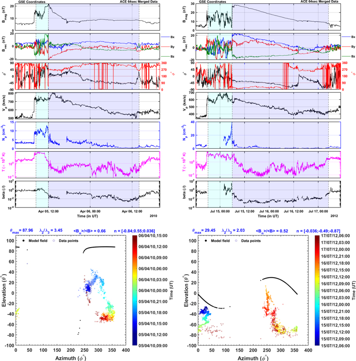
Figure 2. Same as Figure 1 for ICMEs observed by the ACE spacecraft on 2010 April 5 and 2012 July 14, respectively.
Download figure:
Standard image High-resolution image3.1. PMS Molded ICME MCs
Figure 1 presents examples of two ICMEs observed on 2013 July 12 (left) and 2014 August 19 (right). The boundary of the MC associated with 2013 July 12 ranges from 2013 July 13 at 04:59 UT to 2014 July 14 at 23:59 UT. Similarly, for the 2014 August 19 MC, the MC boundary starts on 2014 August 19 at 15:59 UT and ends on 2014 August 21 at 04:59 UT. The average plasma parameters associated with the 2013 July 12 MC are Bmag = 12.28 nT, Vp = 403.79 km s−1, Tp = 16,228.57 K, Np = 3.69 cm3, β = 0.02, Pmag = 0.062 nPa, and Pth = 0.001 nPa. Similarly, during the 2014 August 19 ICME MC the average plasma parameters are Bmag = 16.55 nT, Vp = 360.77 km s−1, Tp = 31,073.92 K, Np = 6.88 cm3, β = 0.04, Pmag = 0.114 nPa, and Pth = 0.004 nPa, respectively.
Further, we applied a PMS analysis test to these two ICMEs. The bottom plots in Figure 1 show the typical distribution of θ and ϕ of the above two MCs. We clearly observed that it shows a nice wavy distribution of θ and ϕ, which is one of the typical signatures of PMS (Nakagawa et al. 1989; Jones & Balogh 2000; Kataoka et al. 2015; Shaikh et al. 2020). To conform it, an additional test has been performed, namely (see Section 2), the estimation of planarity (∣Bn
∣/ 〈 B 〉) and efficiency (λ2/λ3). We observe that ∣Bn
∣/ 〈 B 〉 = 0.10 and λ2/λ3 = 10.80 during the 2013 July 12 ICME MC, while 0.11 and 32.57 for the 2014 August 19 ICME MC. Thus, both MCs satisfy all the essential and necessary criteria needed for a structure to be PMS (Nakagawa et al. 1989; Neugebauer et al. 1993; Jones et al. 1999; Shaikh et al. 2018). Moreover, the inclination ( ) with respect to the ecliptic plane and normal direction (
n
) of the PMS plane associated with the 2013 July 12 ICME MC is
) with respect to the ecliptic plane and normal direction (
n
) of the PMS plane associated with the 2013 July 12 ICME MC is  and
n
= (−0.96, −0.28, −0.091), while it is
and
n
= (−0.96, −0.28, −0.091), while it is  and
n
= (0.92, −0.044, −0.38) for the 2014 August 19 ICME MC, respectively.
and
n
= (0.92, −0.044, −0.38) for the 2014 August 19 ICME MC, respectively.
3.2. Non-PMS Molded ICME MCs
Figure 2 is similar to Figure 1 but for the case of ICME MCs, which do not show characteristics of PMS. The left and right plots in Figure 2 correspond to ICME observed on 2010 April 5 and 2012 July 14, respectively. The boundary of the ICME MC observed on 2010 April 5 ranges from 2010 April 5 at 11:59 UT to 2010 April 6 at 14:00 UT, while for the ICME observed on 2012 July 14, the MC starts on 2012 July 15 at 06:00 UT and ends on 2012 July 17 at 05:00 UT, respectively. The average plasma parameters of the 2010 April 5 ICME MC are Bmag = 9.24 nT, Vp = 633.69 km s−1, Tp = 50,539.32 K, Np = 2.22 cm3, β = 0.07, Pmag = 0.037 nPa, and Pth = 0.002 nPa, while for the case of the 2012 July 14 ICME MC, Bmag = 16.64 nT, Vp = 481.92 km s−1, Tp = 48,923.30 K, Np = 1.62 cm3, β = 0.01, Pmag = 0.127 nPa, and Pth = 0.002 nPa, respectively.
Similar to Section 3.1, the bottom plots in Figure 2 demonstrate the PMS analysis test for the above two ICME MCs. We clearly observed that the distribution of θ versus ϕ plot does not show a wavy pattern, which hints that these MCs could not have PMS characteristics. Moreover, for the case of the 2010 April 5 ICME MC, we noted that ∣Bn ∣/ 〈 B 〉 = 0.66 and λ2/λ3 = 3.45, while for the 2012 July 14 ICME MC ∣Bn ∣/ 〈 B 〉 = 0.52 and λ2/λ3 = 2.03, respectively. Thus, these two MCs do not show any signatures of PMS; hence, these are not PMS (Nakagawa et al. 1989; Neugebauer et al. 1993; Shaikh et al. 2018).
We have applied the PMS test to the studied 469 ICME MC/N-MC boundaries (note that we have not included the ICME sheath part in the analysis). The analysis suggests that 136 (i.e., ∼29%) ICME MCs/N-MCs show PMS characteristics, whereas 333 (i.e., ∼71%) do not exhibit PMS features. Thus, we observe that ICME MCs/N-MCs have two distinct features; (1) ICME MCs/N-MCs that exhibit PMS characteristics shall hereafter be referred to as planar ICMEs for convenience, and (2) ICME MCs/N-MCs that do not display a PMS signature are referred to as nonplanar ICMEs going forward for convenience. Furthermore, the detailed averaged plasma properties of planar and nonplanar ICMEs are given in Appendices A and B as two separate tables: Table 1, showing planar ICMEs, and Table 2, showing nonplanar ICMEs. It is worth noting that the values of Bn for both forms of ICMEs are not considerably different, implying that identifying planar and nonplanar structures would require a greater total B of planar ICMEs than nonplanar ICMEs. These features of ICMEs are associated with the geometric morphology of ICMEs in interplanetary space. Their average plasma properties are discussed in Section 4.
4. Average Plasma Characteristics of Planar and Nonplanar ICMEs
Statistical analysis of the different plasma parameters like total IMF Bmag, Bzmin, Bzmax, and plasma speed Vp , temperature Tp , density Np , beta β, thermal pressure Pth, and magnetic pressure Pmag has been performed for the case of 136 planar ICMEs and 333 nonplanar ICMEs. The complete list of planar and nonplanar ICMEs, and averaged values of the aforementioned plasma parameters are listed in Appendices A and B.
4.1. Total IMF Bmag
Panel (a) in Figure 3 represents the right-skewed distribution of average Bmag for both planar and nonplanar ICMEs. In the case of planar ICMEs, the mean and median of the averaged Bmag are estimated as 12.20 and 11.04 nT, while for the nonplanar ICMEs, 8.66 and 8.10 nT, respectively. It implies that the average and the median value of Bmag are about 40.88% and 36.30% higher in planar ICMEs than Nonplanar ICMEs, i.e., planar ICMEs are magnetically stronger than nonplanar ICMEs. It suggests comparing Bn for planar and nonplanar ICMEs as well.

Figure 3. Normalized distribution of average magnetic field and plasma parameters in planar sheaths and nonplanar ICMEs.
Download figure:
Standard image High-resolution image4.2. Southward (Bzmin) and Northward (Bzmax) IMF
The left-skewed distribution of IMF Bzmin and Bzmax associated with planar and nonplanar ICMEs are shown in Figures 3(b) and (c). The average strength of Bzmin and Bzmax in planar ICMEs are −13.67 and 13.10 nT, while median values are −11.33 and 11.48, respectively. It indicates that in the case of Bzmin, the mean and median values are 44.50% and 44.88% higher, while in the case of Bzmax, 47.36% and 48.70% higher in planar ICMEs in comparison to nonplanar ICMEs. It indicates that the strength of IMF Bz (southward or northward) within planar ICMEs is much stronger than in nonplanar ICMEs. It suggests that planar ICMEs are more geoeffective than nonplanar ICMEs.
4.3. Plasma: Vp and Tp
The subplots in Figures 3(d) and (e) show the distribution of averaged solar wind speed for the planar and nonplanar ICMEs regions. Interestingly, we observe that both types of ICMEs show a right-skewed distribution. The mean and median of velocity distribution for planar and nonplanar ICMEs are 451.79 and 424.20 km s−1 and 458.95 and 439.06 km s−1, respectively. Similarly, the temperature distribution shows 0.51 × 10⁵ and 0.36 × 10⁵ K and 0.52 × 10⁵ and 0.38 × 10⁵ K, respectively. Surprisingly, we observe that the Vp and Tp values do not show any significant difference between planar and nonplanar ICMEs. We anticipate that the ICME speed will eventually be close to the solar wind speed due to the drag effect of the solar wind. Unless planar and nonplanar ICMEs are in very different solar wind conditions or have significantly different start speeds, their speeds around 1 au may not be significantly different.
4.4. Plasma: β, Pmag, and Pth
The subplot in Figure 3(f) demonstrates that the nature of the averaged β distribution is right-skewed for planar and nonplanar ICMEs. For planar ICMEs the distribution mean and median values are 0.14 and 0.11, while they are 0.19 and 0.13 for nonplanar ICMEs. From a β point of view, we observe a 35.71% increment in nonplanar ICMEs compared to planar ICMEs, which implies that planar ICMEs have a low plasma beta value.
Furthermore, the subplots in Figures 3(g) and (h) represent the right-skewed distribution of average magnetic (Pmag) and thermal (Pth) pressure during planar and nonplanar ICMEs. During the distribution of planar ICMEs, the mean values are Pth = 0.006 nPa and Pmag = 0.08 nPa; however, for nonplanar ICMEs, the mean values are noted as Pth = 0.004 and Pmag = 0.04 nPa, respectively. This suggests that Pth and Pmag show ∼50% and 100% increments during planar ICMEs as compared to nonplanar ICMEs. However, the median of Pth and Pmag represents 33.33% and 66.66% increments during planar ICMEs with respect to nonplanar ICMEs. Thus, we observe that Pth and Pmag are significantly higher during planar ICMEs; however, their ratio is balanced such that the β shows an increment during nonplanar ICMEs.
4.5. Plasma Np
The average plasma density during both types of ICMEs represents a right-skewed distribution. The mean and median of the distribution of planar and nonplanar ICMEs are 8.40 and 7.88 cm−3 and 6.22 and 5.21 cm−3, respectively. The observation shows that planar ICMEs have nearly 35% increased density than nonplanar ICMEs (for mean values). However, we observe a 51.24% increment in median value during planar ICMEs. Thus, we conclude that planar ICMEs are denser as compared to nonplanar ICMEs.
4.6. Thickness and Duration of ICME
The top left plot in Figure 4 shows the right-skewed distribution of the thickness of planar and nonplanar ICMEs. We estimated the thickness of ICMEs by multiplying the time duration of the ICMEs' transit with the average speed of the ICMEs. We observe that the mean and median of the distribution of planar ICMEs are 0.26 au and 0.23 au; however, for the case of nonplanar ICMEs, it is 0.32 au and 0.28 au, respectively. This indicates that the thickness of planar ICMEs is ∼23% less compared to nonplanar ICMEs. The median values indicate a 21.74% decrease in ICMEs' thickness during planar as compared to nonplanar ICMEs. Similarly, the top-right plot in Figure 4 demonstrates the right-skewed distribution of ICMEs duration. Interestingly, we observe that the mean and median of the distribution show an 18.69% decrease in the duration of planar ICMEs compared to nonplanar ICMEs. Thus, the thickness and duration of planar ICMEs are less compared to nonplanar ICMEs.
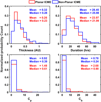
Figure 4. Normalized distribution of thickness, duration, density, and magnetic compressibility in planar and nonplanar ICMEs.
Download figure:
Standard image High-resolution image4.7. Density and Magnetic Compressibility
The bottom left and right plots in Figure 4 demonstrate the average of density ![${C}_{p}=\tfrac{\delta {N}_{p}^{2}}{{[{({N}_{p})}_{\mathrm{avg}}]}^{2}}$](https://content.cld.iop.org/journals/0004-637X/938/2/146/revision1/apjac8f2bieqn19.gif) and magnetic
and magnetic ![${C}_{b}=\tfrac{\delta {B}^{2}}{{[{(B)}_{\mathrm{avg}}]}^{2}}$](https://content.cld.iop.org/journals/0004-637X/938/2/146/revision1/apjac8f2bieqn20.gif) compressibility distribution of planar and nonplanar ICMEs. Here,
compressibility distribution of planar and nonplanar ICMEs. Here,  , and δ
B = B − (B)avg, where
, and δ
B = B − (B)avg, where  and (B)avg are average values within planar and nonplanar ICMEs. An analysis shows that the nature of the distribution is right-skewed distribution. The mean value of the distribution indicates that Cp
in planar ICMEs is about 1.61 times higher than in nonplanar ICMEs. Similarly, we observe a 3.44 times increase in Cb
within planar ICMEs as compared to nonplanar ICMEs. This analysis indicates that Cp
and Cb
within planar ICMEs are significantly higher than in nonplanar ICMEs. As a result, planar ICMEs are more compressed than nonplanar ICMEs. In this regard, we feel that the suggested analysis can be strengthened by estimating, for example, the density compression ratio at the leading edge of planar and nonplanar ICMEs, the total pressure within and outside the planet and nonplanar ICMEs, and/or the expansion speed. These computations, however, are not provided in this study. Furthermore, we will include the additional calculations in our next paper.
and (B)avg are average values within planar and nonplanar ICMEs. An analysis shows that the nature of the distribution is right-skewed distribution. The mean value of the distribution indicates that Cp
in planar ICMEs is about 1.61 times higher than in nonplanar ICMEs. Similarly, we observe a 3.44 times increase in Cb
within planar ICMEs as compared to nonplanar ICMEs. This analysis indicates that Cp
and Cb
within planar ICMEs are significantly higher than in nonplanar ICMEs. As a result, planar ICMEs are more compressed than nonplanar ICMEs. In this regard, we feel that the suggested analysis can be strengthened by estimating, for example, the density compression ratio at the leading edge of planar and nonplanar ICMEs, the total pressure within and outside the planet and nonplanar ICMEs, and/or the expansion speed. These computations, however, are not provided in this study. Furthermore, we will include the additional calculations in our next paper.
4.8. Orientation of Planar and Nonplanar ICMEs
Since we have applied MVA to the ICME MC/EJ magnetic field data, it is important to discuss the orientation of ICME MCs/N-MCs axes (see, for example, Klein & Burlaga 1982; Bothmer & Schwenn 1998; Sonnerup & Scheible 1998), i.e., elevation/inclination  and azimuth orientation
  , where e2 is the intermediate eigenvector, see Section 2 for more details. The top plots in Figure 5 demonstrate the distribution of θaxes and ϕaxes for planar and nonplanar ICMEs. The top left plot clearly shows that distributions of ϕaxes have two different peaks, one between 90° and 120° and another between 240° and 270° for both types of ICMEs, respectively. It is interesting to see that the mean value of ϕaxes during planar and nonplanar ICMEs are ϕaxes = 168
 69 and 18584, whereas, the median values are 14513 and 19391, respectively. Thus, on average, we observe about a 17° difference in the axial orientation of planar and nonplanar ICMEs. Therefore, it is surprising to see that the azimuth orientation of planar ICMEs axes is toward the eastward direction, whereas, the nonplanar ICMEs axes are oriented in a slightly westward direction. Moreover, the right plot in Figure 5 shows the left-skewed distribution of the inclination angle (θaxes) for both planar and nonplanar ICMEs. We observe a similar profile in the case of planar and nonplanar ICMEs. The mean and median values of the θaxes for northward(θaxes < 0) and southward (θaxes > 0) oriented planar ICMEs are 4149 and −3043 and 4308 and −2493, respectively. Whereas in the case of nonplanar ICMEs the mean and median values of the northward and southward orientations are 3625 and −3332 and 3269 and −2816, respectively. Thus, from Figure 5, it can be seen that (1) for planar ICMEs, the inclination angle tends to point toward the north, and (2) for nonplanar ICMEs, the axis tends to lie in the ecliptic plane though slightly northward. Such a slight difference in the azimuth and elevation orientation of planar and nonplanar ICMEs could be due to the limitation of the MVA method itself (e.g., Rosa Oliveira et al. 2021, and references therein). Therefore, we need better models to correctly estimate the axial orientation of planar and nonplanar ICMEs.
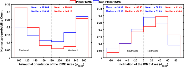
Figure 5. Normalized distribution of the orientation (elevation/inclination: θaxes and azimuth: ϕaxes angle) of planar and nonplanar ICMEs axes. The vertical dashed line in the left plot separates the eastward and westward directions, whereas in the right plot it separates southward and northward inclined oriented ICME axes.
Download figure:
Standard image High-resolution image4.9. Pearson Correlation Analysis
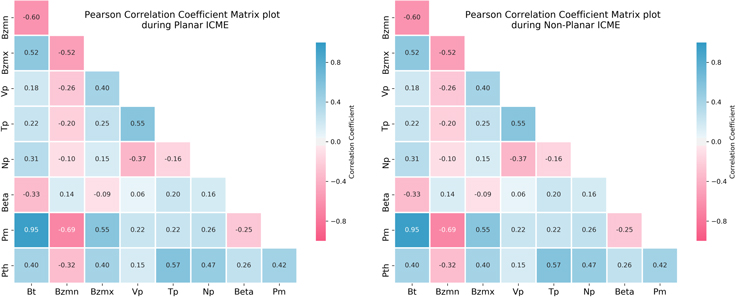
The left and right plots in Figure 6 illustrate the Pearson correlation coefficient (CC) analysis matrix between different plasma parameters for planar and nonplanar ICMEs. The values and color scale in Figure 6 indicate the extent of correlation between the variables. When CC ≤ 0.5 or CC ≥ −0.5 between any two plasma parameters, it indicates that variables are poorly dependent on each other. However, CC ≥ 0.5 or CC ≤ −0.5 indicates a high dependency of variables on each other.
In the case of planar ICMEs, from the left plot, we can observe a significantly high CC between the following variables: Vp and Tp is 0.58, Bzmn and Bt is −0.76 and Bzmx and Bt is 0.74, Pm and Bt is 0.94, Pth and Bt is 0.56, Bzmn and Bmx is −0.69, Pm and Bmn is −0.84, Pm and Bmx is 0.72, Pth and Bmx is 0.60, and Pth and Tp is 0.64, respectively. Similarly, during nonplanar ICMEs, the CC is significantly high for the following variables: Vp and Tp is 0.55, Bzmn and Bt is -0.60 and Bzmx and Bt is 0.52, Pm and Bt is 0.95, Bzmn and Bmx is −0.52, Pm and Bmn is −0.69, Pm and Bmx is 0.55, and Pth and Tp is 0.57, respectively. Thus, we clearly observe that plasma variables are highly correlated in planar ICMEs compare to nonplanar ICMEs (see Figure 6).
5. Discussion and Conclusion
In general, ICME MCs/N-MCs are examined or evaluated in three methods, including (i) theoretical study to investigate the geometry of the magnetic structure (e.g., Farrugia et al. 1995), (ii) numerical methods for the magnetic field topology (e.g., Hu & Sonnerup 2001; Vandas & Romashets 2003), and (iii) analytical models that assume cloud topologies (e.g., Marubashi & Lepping 2007; Démoulin & Dasso 2009b). All of these methodologies were designed to examine and recreate ICME MC/N-MC magnetic field line structure using interplanetary spacecraft observations. Furthermore, the MVA approach is a widely used methodology for finding the direction of the MC/N-MC axes. (e.g., Lepping & Behannon 1980; Bothmer & Rust 1997; Bothmer & Schwenn 1998; Sonnerup & Scheible 1998). The MVA approach is based on determining the magnetic field's eigenvalues and related eigenvectors. The validity of the MVA application is determined by the ratio of the intermediate (λ2) and minimum (λ3) eigenvalues. The direction of the ICME (MC/N-MC) axis is given by the intermediate eigenvector. The MVA approach has been utilized in several studies to identify the orientation (latitude and longitude of the ICME main axis) and configuration (hodogram analysis) of ICMEs (Klein & Burlaga 1982; Bothmer & Schwenn 1998; Farrugia et al. 1999; Gulisano et al. 2005).
Furthermore, the MVA approach is used to determine the PMS characteristics of the examined region (Nakagawa et al. 1989; Neugebauer et al. 1993; Rosa Oliveira et al. 2020; Shaikh et al. 2020). We can use PMS analysis criteria for the ICME (MC/N-MC) if and only if the eigenvalues are well separated, and the magnetic field in the normal direction (Bn ) is low, and there is a clear rotation of the azimuth angle. This implies that ICMEs show the signature of a quasi-2D structure with an invariance along the intermediate eigenvector direction, and the magnetic field rotates in the plane of the ICME cross section. Burlaga et al. (1981) suggest that the ICME magnetic field is highly organized on a large scale and shows a planar signature (i.e., magnetic field vectors are in the plane or parallel to a plane). However, for a structure to be PMS, the ϕ − θ space should show IMF distributed over the full range of ϕ in addition to the magnetic field vectors should be in a plane (Nakagawa et al. 1989; Nakagawa 1993; Neugebauer et al. 1993; Palmerio et al. 2016; Shaikh et al. 2020). Moreover, Nakagawa et al. (1989) suggest that ICME will not show PMS characteristics; however, ICME can demonstrate the confinement of magnetic field vectors to a plane. Thus, it implies that PMS is a distinct magnetic structure in the heliosphere, quasi-2D in nature.
We analyzed 469 ICMEs in detail and applied the PMS analysis test to these ICMEs in the present statistical study. Our investigation explicitly suggests that about ∼29% (136 ICME MCs/N-MCs) show PMS characteristics, whereas about 71% (333 ICME MCs/N-MCs) do not show any PMS signature. We applied the PMS analysis test to the entire ICME MCs/N-MCs, i.e., not in parts. We discovered that the duration of ICME MCs/N-MCs that were converted into PMS ranged from ∼4.0 to ∼63 hr, with an average duration of ∼23.97 hr. We also computed the thickness of the ICMEs by multiplying their duration by their average speed. We discovered that the thickness of planar ICMEs varies between ∼0.041 and ∼0.68 au, with an average thickness of ∼0.27 au. Nonplanar ICMEs, on the other hand, have an average duration and thickness of ∼28.45 hr and ∼0.32 au. Figure 4 clearly depicts that planar ICMEs are thinner than nonplanar ICMEs. Our study also shows that planar ICMEs have much higher density and magnetic compressibility than nonplanar ICMEs. It implies that compression is important in turning ICMEs into a PMS structure, i.e., a quasi-2D magnetic structure.
Figure 6. Pearson CC between the IMF and different plasma parameters for planar and nonplanar MCs. Note that, Bzmn and Bzmx are the same as Bzmin and Bzmax.
Download figure:
Standard image High-resolution image
In addition, our study also suggests that the strength of the total IMF, i.e., Bmag, southward (Bzmin), northward (Bzmax), plasma beta (β), magnetic (Pmag) and thermal (Pth) pressure, and plasma density (Np ) is significantly greater in PMS molded ICMEs than nonplanar ICMEs. It also suggests that high compression could cause this additional increase in plasma parameters in planar ICMEs compared to nonplanar ICMEs as IMF Bz orientation and strength play a crucial role in geomagnetic storms. Thus, our results propose that planar ICMEs are more favorable for a geomagnetic storm. A decade-long study indicates that strong IMF Bz (southward) and northward geomagnetic field lines reconnect and transfer energy, mass, and momentum from the solar wind flow to the magnetosphere (Dungey 1961; Akasofu 1981; Nishida 1983). Several studies indicate that PMS molded regions contribute significantly to substantial space weather effects on Earth compared to non-PMS regions (Kataoka et al. 2015; Palmerio et al. 2016; Shaikh et al. 2018). As a result, we anticipate that planar ICMEs will be more favorable to geoeffective space weather than nonplanar ICMEs. Moreover, planar ICMEs do not show any significant increase in the following plasma parameters: plasma speed (Vp ) and plasma temperature (Tp ). This implies that there is no additional heating inside planar ICMEs, which contradicts the PMS plasma characteristic associated with the ICME sheath (Palmerio et al. 2016; Shaikh et al. 2020). Furthermore, the correlation between plasma temperature and velocity in planar ICMEs is 0.58, while 0.55 in nonplanar ICMEs indicates that the dependency of plasma temperature on velocity is almost the same in planar and nonplanar ICMEs. Moreover, we observe that Pth and Pmag show 50% and 100% increments during planar ICMEs compared to nonplanar ICMEs; however, the β shows a 35.71% increment during nonplanar ICMEs. This indicates that high compression in planar ICMEs could be the reason for such increment. It is important to note that, from the literature, we know that compression causes heating of the plasma; however, in PMS molded ICMEs, we do not observe any significant heating effect. A further detailed study is needed to understand the role of compression in plasma heating. The deformation and compression of ICMEs can be caused due to the following reasons: (i) interaction of ICME with a high-speed stream (HSS) either from the front side or from behind (Winslow et al. 2016; Heinemann et al. 2019), (ii) ICME-ICME interaction (Lugaz et al. 2017), (iii) interaction between ICME and a corotating interaction region or stream interaction region (Al-Shakarchi 2018), (iv) interaction of ICME with another large-scale magnetic structure (such as a heliospheric current sheet) or with the solar wind, etc.
The deformation of the ICMEs and their cross section has been studied by many researchers in the past (e.g., Hidalgo et al. 2002a, 2002b; Al-Haddad et al. 2013; Shiota & Kataoka 2016). It has been observed that ICME (MC/flux rope) deforms in many ways, such as kinking or rotation (Isavnin et al. 2013), eroding due to reconnection (Wang et al. 2018), deflection (Zhuang et al. 2019), compression (due to ICMEHSS interaction) (Winslow et al. 2016; He et al. 2018), pancaking (Isavnin 2016), etc. All these deformations vary from close to the Sun to interplanetary space (Nieves-Chinchilla et al. 2012; Winslow et al. 2016). Moreover, our proposed new morphology of ICMEs, i.e., PMS molded ICMEs provide new insight into the global geometry of ICMEs. Thus, detailed analysis is needed to reveal a kaleidoscope view of ICME morphology or geometry. All these effects associated with ICME geometry/morphology alter the initial ICME properties observed close to the Sun to interplanetary space, making predictions of arrival time and geoeffectiveness a complex endeavor (Richardson et al. 2018; Möstl et al. 2020). Our study also emphasizes that it is essential to investigate solar wind's role in ICME propagation, deformation, and interaction from close to the Sun to 1 au in distance.
We would like to draw the reader's attention to the fact that ICME may or may or may not have MC properties (Chi et al. 2016); Richardson & Cane 2010). We closely monitored the list of published ICME 8 and examine our studied ICME MCs/N-MCs (136) that turned into PMS. We found that out of 136 (29%) planar ICMEs, 69 (50.74%) have an ideal MC profile, and 67 (49.26%) are N-MCs. 9 Furthermore, out of 333 nonplanar ICME MCs/N-MCs, 88 (26.43%) are MCs while the remaining 245 (73.57%) are N-MCs. Note that the number of ICME MCs can vary depending on the catalog used in the study; here, we use the ICME catalog available on the ACE database. Thus, whether an ICME has an ideal MC-like configuration or not, it may be converted into a PMS. As a result, our findings are significant in understanding the morphological alterations in ICMEs. Moreover, we also observe that planar ICMEs are oriented toward the eastward direction whereas nonplanar ICMEs are slightly oriented toward the westward direction. Furthermore, planar ICMEs axes are inclined more northward, while nonplanar ICMEs axes tend to lie in the ecliptic plane in a slightly northward direction.
In conclusion, our study unambiguously depicts that planar ICMEs are magnetically stronger than nonplanar ICMEs. Also, high southward/northward IMF associated with planar ICMEs may have strong geoeffectiveness compared to nonplanar ICMEs. Moreover, a considerably high number density, thermal pressure, magnetic pressure, density, and magnetic compressibility within planar ICMEs suggest that compression could be the causative agent. In addition, significantly narrow (thickness and duration) planar ICMEs support the compression hypothesis for converting ICME MCs/N-MCs into PMSs. As a result, we assume that ICME MCs/N-MCs are compressed to the point where their concentric cylindrical surfaces (with a circular cross section) are crushed to elliptical surface layers, resulting in the observed PMS molded ICME MCs/N-MCs, i.e., planar ICMEs (Raghav & Shaikh 2020). The aspect ratio of planar ICMEs will be altered at a higher value throughout this operation. We argued that such high compression is conceivable as a result of ICMEs interacting with rapid solar wind or another ICME/CIR. As a result, the above work offers an opportunity to comprehend the deformation of ICMEs utilizing in situ data from interplanetary space. Our study will play a vital role in the predictability of space weather phenomena.
The authors would like to acknowledge all individuals involved with ACE spacecraft mission development, the team that provided the data, etc. We also acknowledge the NASA/GSFC's Space Physics Data Facilities (CDAWeb or ftp) service. Z.S. also thanks "The Department of Science and Technology (DST)", the Government of India, for their support (https://dst.gov.in/). We acknowledge SERB, India, as A.R. is supported by SERB project reference file number CRG/2020/002314.
Software: MATLAB (https://in.mathworks.com/products/matlab.html), Python (NumPy (Van Der Walt et al. 2011; Harris et al. 2020), Matplotlib (Hunter & Dale 2007), Seaborn (Waskom et al. 2016)).
Appendix A: List of Planar ICME MC Events and Their Plasma Properties
Here, we list the 136 ICME events that show PMS characteristics referred to as planar ICMEs. We found that out of 136 planar ICMEs, 69 (50.74%) have an ideal MC profile and 67 (49.26%) are N-MCs (see the list of ICMEs on the ACE website). Table 1 shows the average plasma properties as well as the magnetic field strength. A description of each column is provided at the bottom of the table.
Table 1. List of Planar ICME MC/N-MCs from 1998–2017
| MC/N-MC onset | MC/N-MC End | n | λ |

|

| Bmag | Bzmin | Bzmax | Vp | Tp | Np | β | Pmag | Pth |

|

| MC? | ||||
|---|---|---|---|---|---|---|---|---|---|---|---|---|---|---|---|---|---|---|---|---|---|
| (Date and Time) | (Date and Time) | nx | ny | nz | λ1 | λ2 | λ3 | (nT) | (nT) | (nT) | (km s−1) | (K) | (cm−3) | nPa | nPa | (◦) | |||||
| (1) | (2) | (3) | (4) | (5) | (6) | (7) | (8) | (9) | (10) | (11) | (12) | (13) | (14) | (15) | (16) | (17) | (18) | (19) | (20) | (21) | (22) |
| 1998 Jan 29 20:00 | 1998 Jan 31 00:59 | −0.94 | −0.31 | −0.14 | 18.76 | 6.15 | 0.65 | 3.05 | 9.39 | 7.91 | −7.91 | 7.54 | ⋯ | ⋯ | ⋯ | ⋯ | 0.025 | ⋯ | 0.22 | 77.22 | no |
| 1998 Apr 3 12:59 | 1998 Mar 6 8:59 | −0.90 | −0.29 | −0.33 | 33.73 | 18.09 | 0.96 | 1.86 | 18.89 | 9.97 | −9.16 | 9.73 | 341.45 | 17629.34 | 15.64 | 0.31 | 0.042 | 0.004 | 0.08 | 70.82 | yes |
| 1998 Mar 25 12:59 | 1998 Mar 26 10:00 | −0.84 | −0.37 | 0.38 | 38.17 | 18.04 | 4.62 | 2.12 | 3.90 | 10.34 | −8.37 | 10.27 | 405.89 | 30783.07 | 15.68 | 0.16 | 0.043 | 0.007 | 0.16 | 67.45 | no |
| 1998 Apr 11 23:00 | 1998 Apr 13 18:00 | 0.84 | 0.14 | −0.52 | 25.38 | 6.90 | 1.78 | 3.68 | 3.87 | 8.00 | −5.81 | 9.64 | 389.92 | 30203.12 | 6.05 | 0.15 | 0.026 | 0.003 | 0.13 | 58.87 | no |
| 1998 Jun 2 10:00 | 1998 Jun 2 18:00 | −0.83 | 0.47 | −0.30 | 24.20 | 7.81 | 0.74 | 3.10 | 10.50 | 9.80 | −7.40 | 8.39 | 399.79 | 36823.48 | 8.61 | 0.15 | 0.039 | 0.005 | 0.13 | 72.43 | yes |
| 2016 Aug 2 14:00 | 2016 Aug 3 03:00 | −0.95 | 0.00 | 0.31 | 165.25 | 36.51 | 5.33 | 4.53 | 6.85 | 19.92 | −13.58 | 20.90 | 424.56 | 34534.59 | ⋯ | ⋯ | 0.161 | ⋯ | 0.08 | 71.91 | yes |
| 2016 Oct 13 06:00 | 2016 Oct 14 15:59 | 0.97 | 0.00 | −0.24 | 156.64 | 55.42 | 3.66 | 2.83 | 15.15 | 19.43 | −20.16 | 14.45 | 386.01 | 34694.25 | 4.35 | 0.02 | 0.154 | 0.002 | 0.11 | 75.04 | yes |
| 2016 Nov 9 23:59 | 2016 Nov 10 15:59 | −0.88 | −0.43 | 0.20 | 39.77 | 15.29 | 4.73 | 2.60 | 3.23 | 11.47 | −10.71 | 11.75 | 360.44 | 30200.86 | 12.86 | 0.18 | 0.053 | 0.007 | 0.15 | 78.72 | yes |
| 2017 Apr 4 04:00 | 2017 Apr 4 13:59 | −1.00 | −0.08 | 0.01 | 78.21 | 13.20 | 2.21 | 5.92 | 5.97 | 13.40 | −13.17 | 12.37 | 415.58 | 39850.69 | 10.59 | 0.13 | 0.073 | 0.007 | 0.20 | 86.79 | yes |
| 2017 Sep 7 19:59 | 2017 Sep 8 03:59 | −0.90 | 0.36 | −0.25 | 160.86 | 65.38 | 6.75 | 2.46 | 9.69 | 16.89 | −32.40 | 14.94 | 625.86 | 402639.88 | 3.36 | 0.06 | 0.137 | 0.013 | 0.18 | 74.75 | no |
Note. The date and time are in the format of year/month/day hour:minutes. n = nx
, ny
, nz
are the normal directions of the plane and λ = (λ1, λ2, λ3) are the eigenvalues of the IMF derived after MVA analysis, respectively. Further, Bmag, Vp
, Tp
, Np
, and β are the average of the total IMF, plasma speed, plasma temperature, plasma number density, and plasma beta. Moreover, Bzmax and Bzmin are the maximum and minimum values of the northward/southward IMF component. The planetary and efficiency of the PMS plane are denoted by  and
and  . The orientation of the PMS plane with respect to the ecliptic plane is given by
  . The last column shows whether the studied regions are MC or not (for the details see https://izw1.caltech.edu/ACE/ASC/DATA/level3/icmetable2.htm).
Only a portion of this table is shown here to demonstrate its form and content. A machine-readable version of the full table is available.
Download table as: DataTypeset image
Appendix B: List of Nonplanar ICME MC/N-MC Events and Their Plasma Properties
Here, we have documented 333 ICME occurrences that exhibit non-PMS features and are referred to be nonplanar ICMEs. Out of 333 nonplanar ICME MCs/N-MCs, 88 (26.43%) are ideal MCs while remaining 245 (73.57%) are N-MCs. Table 2 shows the average plasma properties as well as the magnetic field strength. The information for each column is similar to Table 1.
Table 2. List of Nonplanar ICME MC/N-MCs from 1998–2017
| MC/N-MC onset | MC/N-MC End | n | λ |

|

| Bmag | Bzmin | Bzmax | Vp | Tp | Np | β | Pmag | Pth |

|

| MC? | ||||
|---|---|---|---|---|---|---|---|---|---|---|---|---|---|---|---|---|---|---|---|---|---|
| (Date and Time) | (Date and Time) | nx | ny | nz | λ1 | λ2 | λ3 | (nT) | (nT) | (nT) | (km s−1) | (K) | (cm−3) | nPa | nPa | (°) | |||||
| (1) | (2) | (3) | (4) | (5) | (6) | (7) | (8) | (9) | (10) | (11) | (12) | (13) | (14) | (15) | (16) | (17) | (18) | (19) | (20) | (21) | (22) |
| 1998 Feb 4 04:00 | 1998 Feb 5 23:00 | −0.50 | 0.86 | 0.01 | 25.27 | 22.60 | 0.95 | 1.12 | 23.69 | 10.52 | −9.16 | 6.85 | 303.91 | 14265.60 | 23.77 | 0.19 | 0.047 | 0.005 | 0.57 | 89.52 | yes |
| 1998 Feb 17 09:59 | 1998 Feb 17 20:59 | −0.98 | 0.20 | 0.00 | 27.99 | 8.57 | 3.68 | 3.27 | 2.33 | 12.24 | −13.41 | 7.22 | 399.61 | 30954.39 | 12.43 | 0.10 | 0.060 | 0.006 | 0.40 | 89.76 | yes |
| 1998 Feb 19 00:59 | 1998 Feb 20 00:00 | −0.65 | 0.76 | 0.01 | 26.69 | 1.89 | 0.82 | 14.12 | 2.32 | 8.45 | −6.45 | 11.45 | 437.20 | 60661.83 | 1.92 | 0.07 | 0.029 | 0.002 | 0.78 | 89.21 | no |
| 1998 Mar 31 11:00 | 1998 Apr 3 02:00 | −0.40 | 0.11 | −0.91 | 12.44 | 3.95 | 1.92 | 3.15 | 2.06 | 6.44 | −3.38 | 6.07 | 359.00 | 44649.41 | 9.58 | 0.39 | 0.017 | 0.006 | 0.47 | 24.42 | no |
| 1998 May 2 04:59 | 1998 May 42:00 | −0.15 | −0.38 | −0.91 | 43.14 | 20.04 | 7.81 | 2.15 | 2.57 | 9.87 | −14.27 | 3.47 | 523.08 | 35182.86 | 7.35 | 0.13 | 0.043 | 0.004 | 0.41 | 24.23 | yes |
| 2017 May 27 21:59 | 2017 May 29 13:59 | −0.93 | 0.36 | −0.03 | 130.84 | 93.40 | 4.86 | 1.40 | 19.23 | 15.61 | −22.04 | 13.80 | 363.21 | 45403.60 | 7.43 | 0.02 | 0.100 | 0.003 | 0.26 | 88.44 | yes |
| 2017 Jul 16 15:00 | 2017 Jul 17 20:00 | −0.88 | −0.20 | −0.43 | 77.46 | 16.25 | 5.96 | 4.77 | 2.73 | 13.05 | −17.18 | 8.84 | 519.82 | 53288.14 | 3.50 | 0.04 | 0.071 | 0.003 | 0.54 | 2.18 | yes |
| 2017 Aug 22 03:59 | 2017 Aug 23 18:00 | −0.75 | −0.12 | 0.65 | 9.52 | 3.79 | 2.27 | 2.51 | 1.67 | 4.77 | −7.67 | 3.46 | 505.02 | 36181.24 | 5.09 | 0.72 | 0.010 | 0.002 | 0.49 | 49.71 | no |
| 2017 Sep 8 11:00 | 2017 Sep 10 08:59 | −0.86 | −0.47 | −0.20 | 18.98 | 3.74 | 1.20 | 5.07 | 3.13 | 6.10 | −15.99 | 12.32 | 596.46 | 77995.14 | 0.77 | 0.11 | 0.018 | 0.001 | 0.63 | 77.50 | no |
| 2017 Dec 25 23:59 | 2017 Dec 26 03:59 | −0.92 | 0.28 | −0.28 | 5.18 | 1.66 | 0.67 | 3.13 | 2.46 | 6.98 | −7.25 | 5.58 | 474.74 | 50077.48 | 4.42 | 0.15 | 0.020 | 0.003 | 0.75 | −48.72 | no |
Only a portion of this table is shown here to demonstrate its form and content. A machine-readable version of the full table is available.
Download table as: DataTypeset image
Footnotes
- 3
- 4
- 5
- 6
- 7
- 8
- 9
We also compare the PMS transformed ICME MC/N-MC list with the Wind catalog http://space.ustc.edu.cn/dreams/wind_icmes/. We found that out of 136 (29%) planar ICMEs, 55 (40%) have an ideal MC profile, 39 (29%) are N-MCs, and the remaining ICMEs, 42 (31%) are not listed in the USTC Wind ICME catalog (Chi et al. 2016).