


Abstract
The origins of the GeV gamma rays from nearby radio galaxies are unknown. Hadronic emission from magnetically arrested disks (MADs) around central black holes is proposed as a possible scenario. Particles are accelerated in a MAD by magnetic reconnection and stochastic turbulence acceleration. We pick out the 15 brightest radio galaxies in the GeV band from The Fourth Catalog of Active Galactic Nuclei Detected by the Fermi Large Area Telescope, Data Release 2 and apply the MAD model. We find that we can explain the data in the GeV bands by the MAD model if the accretion rate is lower than 0.1% of the Eddington rate. For a higher accretion rate, GeV gamma rays are absorbed by two-photon interaction due to copious low-energy photons. If we assume another proposed prescription of the electron-heating rate by magnetic reconnection, the MAD model fails to reproduce the GeV data for the majority of our sample. This indicates that the electron-heating rate is crucial. We also apply the MAD model to Sagittarius A* (Sgr A*) and find that GeV gamma rays observed at the Galactic center do not come from the MAD of Sgr A*. We estimate the cosmic ray (CR) intensity from Sgr A*, but it is too low to explain the high-energy CR intensity on Earth.
Export citation and abstract BibTeX RIS

Original content from this work may be used under the terms of the Creative Commons Attribution 4.0 licence. Any further distribution of this work must maintain attribution to the author(s) and the title of the work, journal citation and DOI.
1. Introduction
Radio-loud active galactic nuclei (AGNs) have powerful relativistic jets that have a strong influence on star formation activities in host galaxies and thermodynamics of gases in galaxy clusters. These AGNs also exhibit broadband nonthermal emission signatures from radio to GeV–TeV gamma rays. However, the production mechanism and physical nature of the jets and the nonthermal emission are still unknown (see, e.g., Blandford et al. 2019 and Hada 2019 for recent reviews).
Blazars, a subclass of radio-loud AGNs seen along the jet axis, provide a dominant contribution to the GeV gamma-ray sky (Ackermann et al. 2015; Abdollahi et al. 2020). Owing to the relativistic beaming effect, emission from the jets dominates over the other emission components. Their rapid variabilities also indicate that the gamma-ray emission site should be as compact as subparsec scales (e.g., Abdo et al. 2011).
Radio galaxies, off-axis counterparts of blazars, are also detected in GeV–TeV gamma rays (e.g., Inoue 2011; Stecker et al. 2019; MAGIC Collaboration et al. 2020; H.E.S.S. Collaboration et al. 2020; de Menezes et al. 2020; Tomar et al. 2021). The gamma-ray production sites for radio galaxies are controversial because relativistic beaming effects should be weaker in these objects. Leptonic compact jet models are actively discussed as a standard scenario (e.g., Abdo et al. 2009; MAGIC Collaboration et al. 2020), but, at least in M87, this scenario failed to reproduce the magnetic field strength estimated by core-shift measurements in the radio bands (Kino et al. 2015; Jiang et al. 2021). If we assume the strong magnetic fields given by the radio observations, the resulting gamma-ray spectra are far below the observed flux (Event Horizon Telescope MWL Science Working Group et al. 2021). This motivates one to investigate other scenarios, such as hadronic jets (Reynoso et al. 2011; MAGIC Collaboration et al. 2020), large-scale jets (Hardcastle & Croston 2011), hybrid jets (Fraija & Marinelli 2016), and black hole (BH) magnetospheres (Hirotani & Pu 2016; Kisaka et al. 2020). However, all the aforementioned scenarios have some difficulties or conflicts with other observations (see Kimura & Toma 2020, and references therein).
Kimura & Toma (2020) proposed hadronic emission in magnetically arrested disks (MADs; Bisnovatyi-Kogan & Ruzmaikin 1974; Narayan et al. 2003) as an alternative scenario. Owing to their strong magnetic fields, MADs can launch powerful relativistic jets via the Blandford–Znajek mechanism (Tchekhovskoy et al. 2011; McKinney et al. 2012; Event Horizon Telescope Collaboration et al. 2019). Thus, the presence of jets implies the existence of strong magnetic fields in the vicinity of the BH, which suggests that reconnection-driven particle acceleration (Hoshino & Lyubarsky 2012; Guo et al. 2020) taking place in the MAD is important. The accelerated protons emit GeV gamma rays via the synchrotron process. This model can reproduce the GeV–TeV gamma-ray data from M87 and NGC 315, but the majority of the GeV-detected radio galaxies are as yet unexplored.
The existence of nonthermal particles in accretion flows is supported in terms of both theory and observations. Recent general relativistic magnetohydrodynamic simulations have revealed that MADs can induce magnetic reconnection in highly magnetized plasmas with the magnetization parameter σ =B2/(4π mp np c2) ≳ 1 (Ball et al. 2018; Ripperda et al. 2020, 2022). These reconnection events very efficiently produce nonthermal particles, according to particle-in-cell simulations (Zenitani & Hoshino 2001; Guo et al. 2016; Zhang et al. 2021). Also, accretion flows are turbulent, under which stochastic acceleration processes may produce nonthermal particles efficiently (Kimura et al. 2016; Comisso & Sironi 2018; Zhdankin et al. 2018; Kimura et al. 2019).
Multiwavelength and multimessenger observations also provide hints of nonthermal signatures in accretion flows. Aartsen et al. (2020) reported a ∼3σ high-energy neutrino signal from NGC 1068, a nearby X-ray bright Seyfert galaxy. This motivates one to consider nonthermal hadronic emissions in accretion flows (Inoue et al. 2019; Murase et al. 2020; Gutiérrez et al. 2021; Kheirandish et al. 2021; Kimura et al. 2021b). GeV gamma-ray detections are also reported from radio-quiet AGNs (Wojaczyński et al. 2015; Abdollahi et al. 2020), indicating nonthermal activity in accretion flows. The flaring activities of Sagittarius A* (Sgr A*) in the infrared and X-rays are also considered as nonthermal phenomena triggered by magnetic reconnection (Dexter et al. 2020; Porth et al. 2021; GRAVITY Collaboration et al. 2021).
In this paper, we investigate the characteristics of radio galaxies that can be explained by the MAD model by applying the model to 15 GeV-loud radio galaxies. We also apply our MAD model to Sgr A* to see whether gamma rays from the Galactic center can originate from the accretion flow. This paper is organized as follows. In Section 2, we describe the MAD model constructed by Kimura & Toma (2020). In Section 3, we classify the radio galaxies by comparing the calculated photon spectra to the gamma-ray data and discuss the characteristics of radio galaxies. We also examine another prescription of the electron-heating rate. In Section 4, we also apply the MAD model to Sgr A* and discuss Sgr A* as a cosmic ray (CR) source. In Section 5, we present our conclusions.
2. Magnetically Arrested Disks Model
We calculate the photon spectra with the MAD model constructed by Kimura & Toma (2020). In this model, particles are accelerated by magnetic reconnection at the edge of the accretion disk (Ball et al. 2018; Ripperda et al. 2020) and turbulence in the accretion disk (Yuan et al. 2003; Kimura et al. 2016, 2019). We consider that plasma is accreted onto a supermassive BH of mass M. The mass accretion rate,  , and the size of emission region, R, are normalized by the Eddington rate and by the gravitational radius, respectively, i.e.,
  and
and  . We use the notation Qx = Q/10X
in cgs units, except for the BH mass, M (M9 = M/[109
M⊙]). This model considers the emission by thermal electrons, nonthermal electrons, nonthermal protons, and secondary electron–positron pairs produced by the Bethe–Heitler process (p + γ → p + e+ + e−) and the two-photon interaction (γ + γ → e+ + e−).
. We use the notation Qx = Q/10X
in cgs units, except for the BH mass, M (M9 = M/[109
M⊙]). This model considers the emission by thermal electrons, nonthermal electrons, nonthermal protons, and secondary electron–positron pairs produced by the Bethe–Heitler process (p + γ → p + e+ + e−) and the two-photon interaction (γ + γ → e+ + e−).
We determine the electron temperature by balancing the electron-heating rate with the cooling rate (see Appendix A). The electron-heating mechanism in MADs has not been established yet (Rowan et al. 2017; Kawazura et al. 2019). We consider that magnetic reconnection is the dominant electron-heating mechanism and use the formalism of Hoshino (2018) as a fiducial prescription. Then, the electron-heating rate is given by
where me
and mp
are the mass of an electron and a proton, respectively,  is the proton-heating rate,
  NT is the fraction of the nonthermal particle energy production rate to the dissipation rate, and dis is the fraction of the dissipation rate to the accretion rate. The thermal energy of electrons is lost by radiation cooling or advection to the BH. For
  higher than
  , given in Appendix A, the radiation cooling balances the heating rate because the cooling rate is efficient owing to the high number density and strong magnetic field. For
  lower than
  , the thermal electrons fall to the central BH before they cool. In this case, the electron temperature is estimated as Te
/Tp
≃ Qe
/Qp
(see Appendix A; see also Kimura et al. 2021a).
, the thermal electrons fall to the central BH before they cool. In this case, the electron temperature is estimated as Te
/Tp
≃ Qe
/Qp
(see Appendix A; see also Kimura et al. 2021a).
As escape processes, we consider infall to the BH and diffusion. The infall timescale is tfall ≈ R/VR
, where VR
= α
VK
/2 is the radial velocity, α is the viscous parameter (Shakura & Sunyaev 1973), and  is the Kepler velocity. The diffusion timescale is tdiff ≈ R2/DR
, where DR
≈ η
ri,L
c/3 is the diffusion coefficient, ri,L
= Ei
/(eB) is the Larmor radius, η
ri,L
is the effective mean free path, η is the numerical factor,
is the Kepler velocity. The diffusion timescale is tdiff ≈ R2/DR
, where DR
≈ η
ri,L
c/3 is the diffusion coefficient, ri,L
= Ei
/(eB) is the Larmor radius, η
ri,L
is the effective mean free path, η is the numerical factor,  is the magnetic field,
  is the mass density, H ∼ (Cs
/VK
)R is the scale height of an accretion disk, Cs
≈ VK
/2 is the sound speed, and β is the plasma beta.
is the mass density, H ∼ (Cs
/VK
)R is the scale height of an accretion disk, Cs
≈ VK
/2 is the sound speed, and β is the plasma beta.
We phenomenologically estimate the acceleration timescale as

where  is the Alfvén velocity. We consider synchrotron cooling as the only cooling process for the primary electrons and secondary electron–positron pairs because the other processes are negligible. We consider proton synchrotron, pp collision (p + p → p + p + π), photomeson production (p + γ → p + π), and the Bethe–Heitler process as the proton-cooling processes. In the range of our investigation, pp collision and photomeson production are inefficient because of the low number density of thermal protons and higher threshold energy for photomeson production than the Bethe–Heitler process.
High-energy protons and photons interact with low-energy photons. In Kimura & Toma (2020), since they consider low  radio galaxies, the photons by thermal electrons are dominant as target photons for the Bethe–Heitler process and the two-photon interaction. For a high
  , the number density of photons produced by nonthermal particles is comparable to or higher than that produced by thermal electrons, and thus we take into account all the photons inside the MAD as target photons for the two-photon interaction and the Bethe–Heitler process. We iteratively calculate the photon and the electron–positron pairs spectra until they converge.
3. Results for Radio Galaxies
3.1. Properties of the Magnetically Arrested Disks Model
We show a typical photon spectrum in the MAD model for M = 109
M⊙ and  in Figure 1. The other parameter values are the same as Kimura & Toma (2020; see Table 1), by which the spectra for M87 and NGC 315 are explained. The thick and thin lines are the photon spectra after and before internal attenuation by the two-photon interaction, respectively. The nonthermal protons emit GeV gamma rays (blue dotted line), the secondary electron–positron pairs via the Bethe–Heitler process emit TeV gamma rays (purple dotted line), and the primary electrons and the secondary electron–positron pairs via the two-photon interaction emit X-rays (yellow dashed and green dotted–dashed lines, respectively), as seen in Figure 1.

Figure 1. A typical broadband photon spectrum in the MAD model for  . The thick and thin lines are the photon spectra after and before internal attenuation by the two-photon interaction, respectively. The solid black, red dashed, green dotted–dashed, yellow dashed, blue dotted, and purple dotted lines are the total luminosity by the MAD model, thermal electrons synchrotron and Comptonization, synchrotron by the secondary electron–positron pairs by the two-photon interaction, primary electrons synchrotron, primary protons synchrotron, and synchrotron by the secondary electron–positron pairs via the Bethe–Heitler process, respectively.
Download figure:
Standard image High-resolution imageTable 1. Our Fiducial Parameter Set, from Kimura & Toma (2020)

| α | β |
NT
|
dis
| η | sinj |
|---|---|---|---|---|---|---|
| 10 | 0.3 | 0.1 | 0.33 | 0.15 | 5 | 1.3 |
Download table as: ASCIITypeset image
Both of the most efficient energy-loss timescales of nonthermal protons at the highest energy range, tsyn and tdiff, have the same dependence,  , so that either of the energy-loss processes dominates over the other in the entire proton energy range. The equality tsyn = tdiff gives the critical mass:
Synchrotron cooling is dominant if M > Mcrit for a given  , while diffusion loss is dominant if M < Mcrit. For a fixed value of M, the magnetic field is stronger for higher
  , which leads to higher synchrotron power. The diffusive escape timescale is longer for higher
  due to a smaller Larmor radius. For the example shown in Figure 1, synchrotron cooling is dominant, i.e., M > Mcrit. We find that this is also the case for the vast majority of radio galaxies in our sample (see Figures 2 and 3).
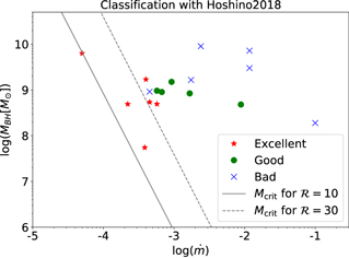
Figure 2. Scatter plot of our sample in the  plane. The red stars, green circles, and blue crosses indicate the "Excellent," "Good," and "Bad" objects, respectively. The solid and dashed lines indicate Mcrit, given by Equation (3), for
  and
and  , respectively.
Download figure:
Standard image High-resolution image
Download figure:
Standard image High-resolution imageAnalytical estimates of the peak energy and luminosity of the proton synchrotron spectrum in the synchrotron-cooling case are given as follows. Because of the hard spectral index of protons, the proton synchrotron spectrum has a peak at the synchrotron frequency for Ep = Ep,cut. Balancing the synchrotron cooling and acceleration timescales, we obtain Ep,cut as
We obtain the peak frequency of the synchrotron spectrum by the nonthermal protons as

Since the synchrotron cooling is the dominant energy-loss timescale, we can approximate that all the energies used for nonthermal proton acceleration are converted to the synchrotron photon energy. Then, the photon luminosity for the proton synchrotron process is estimated to be

We should note that this estimate provides the integrated photon luminosity. The differential photon luminosity given in Figure 1 is lower than Lγ,psyn because of bolometric correction.
3.2. Application to the Various Radio Galaxies
We search for bright radio galaxies in the GeV gamma-ray band from The Fourth Catalog of Active Galactic Nuclei Detected by the Fermi Large Area Telescope, Data Release 2 (Fermi 4LAC-DR2; Ajello et al. 2020). We pick up the 15 brightest objects after excluding Fornax A, M87, and NGC 315. We exclude Fornax A because the gamma-ray emission region is extended and the contribution of the core is lower than 18% (Ackermann et al. 2016). We also omit M87 and NGC 315 since these objects have already been explained in Kimura & Toma (2020). For Centaurus A (Cen A), we use the gamma-ray data of the core while the extended component is also observed. In particular, the High Energy Stereoscopic System (HESS) data (Eγ > 300 GeV) should be from the extended component (H.E.S.S. Collaboration et al. 2020). Then, the 100 GeV data should be the sum of the jet component and disk component. The theoretical model for the HESS data predicts that the extended jet contributes to the 100 GeV data very marginally (H.E.S.S. Collaboration et al. 2020). The MAD contribution to the 100 GeV data is uncertain. Thus, we use the 2–20 GeV data for the fitting procedure and restrict the MAD model not to exceed the data above 100 GeV.
We compare the spectra obtained by the MAD model to the observed ones. To evaluate the goodness of fit, we use the χ2 method. χ2 is a quantity written as

where i represents the observational data points, Fdata,i
is the gamma-ray flux data, Fmodel,i
is the calculated gamma-ray flux, and σi
is the observational error. In this calculation, we use only the gamma-ray data and change only  in the parameters. We consider that the GeV data are explained by the MAD model if Q ≥ 0.01, where Q is the probability that χ2 exceeds the obtained value by Equation (7). We consider that the emission from the jet predominantly contributes to the lower-energy data. The photon flux from radio galaxies shows some variability in all energy bands, and we regard them as the jet contribution. Thus, the contribution by the MAD model should be below the lowest data points in the radio to X-ray bands.
We classify the results into three categories: "Excellent," "Good," and "Bad." We classify objects as "Excellent" if we can explain the gamma-ray data with the parameters in Table 1 and the cataloged value of M. We show the values of M, distance from Earth,  , χ2/ν, and Q for the "Excellent" objects in Appendix B, where ν = N − m is the degree of freedom, N is the number of the data, and m is the number of changing parameters. Since we only change
  , we set m = 1. We also show the photon spectra of these objects in Appendix B. We find that the accretion rates of all the "Excellent" objects are less than 10−3.
For some objects, it is hard to explain the gamma-ray data with the parameters in Table 1 and the cataloged value of M. This is because the GeV gamma rays have been cut off by the two-photon interaction. In order to achieve the high-GeV gamma-ray flux, we may use higher values of  and M. The uncertainty of M is about a factor of 3 (e.g., Kormendy & Ho 2013). We classify objects into "Good" if we can explain the GeV data with
  and M three times higher than the cataloged value. We only change
  during the fitting procedure. Thus, we calculate Q with m = 1. We show the resulting quantities and the photon spectra for the "Good" objects in Appendix B. The accretion rates of the "Good" objects are around 10−3. Owing to the larger emission region, absorption by the two-photon interaction is suppressed, which enables the MAD model to explain GeV data for
  .
.
The remaining objects are classified as "Bad." We show the photon spectra for the "Bad" objects and the quantities for these spectra in Appendix B. There are two types of "Bad" objects. One type has a cutoff due to the two-photon interaction below the GeV energy, which leads to a mismatch in the multi-GeV data. The other type has luminous synchrotron emission by secondary electron–positron pairs via the two-photon interaction, which overshoots the X-ray data.
To see the features of the radio galaxies, we plot M and  for the objects of the three classes in Figure 2, where values of M and
  for individual objects are tabulated in tables in Appendix B. As can be seen, we can explain the gamma-ray data by the MAD model if
  is lower than 10−3. The number density of low-energy photons is higher for a higher
  , and then the two-photon interaction is more efficient. Thus, the photon spectra by the MAD model have the cutoff below the GeV range, and we cannot explain the gamma-ray data for a higher
  . For the jet model, GeV gamma-ray absorption is inefficient owing to the large emission region, and thus we consider that the GeV gamma rays come from the jet for high-
 radio galaxies.
3.3. Another Formalism of the Electron-heating Rate
The electron-heating rate by magnetic reconnection has not yet been established. We also examine another prescription of the electron-heating rate given by Chael et al. (2018):

where  . We show the photon spectra and the resulting quantities of the objects in Appendix C. We calculate the photon spectra for all the objects with this electron-heating rate and classify them as we have done in Section 3.2 by changing
  with the same parameter set. The classification results are shown in Figure 3, where we see that all the classes (Excellent, Good, Bad) equally scatter in the M–
 plane. We find that Qe
/Qp
∼ 0.3 if we use Equation (8) with the parameters in Table 1. On the other hand, Qe
/Qp
∼ 0.07 by Equation (1). The value of Qe
/Qp
corresponds to the luminosity of the electrons, and thus the luminosities in the radio and X-ray bands are high if we use Equation (8). This causes the model flux to overshoot the radio and X-ray data if we adjust
plane. We find that Qe
/Qp
∼ 0.3 if we use Equation (8) with the parameters in Table 1. On the other hand, Qe
/Qp
∼ 0.07 by Equation (1). The value of Qe
/Qp
corresponds to the luminosity of the electrons, and thus the luminosities in the radio and X-ray bands are high if we use Equation (8). This causes the model flux to overshoot the radio and X-ray data if we adjust  so that the resulting gamma-ray spectra match the GeV data. Equation (8) leads to 0.2 < Qe
/Qp
< 0.4 for 5 ≤ r ≤ 30 and 0.01 ≤ β ≤ 1. Thus, we cannot reconcile the results in Section 3.2 even with a different parameter set. This indicates that the electron-heating rate is crucial to explain the gamma-ray data by the MAD model.
so that the resulting gamma-ray spectra match the GeV data. Equation (8) leads to 0.2 < Qe
/Qp
< 0.4 for 5 ≤ r ≤ 30 and 0.01 ≤ β ≤ 1. Thus, we cannot reconcile the results in Section 3.2 even with a different parameter set. This indicates that the electron-heating rate is crucial to explain the gamma-ray data by the MAD model.
4. Sagittarius A*
Observations in the radio and X-ray bands imply that Sgr A* at the Galactic center has a hot accretion flow (Narayan et al. 1995; Manmoto et al. 1997; Yuan et al. 2003; GRAVITY Collaboration et al. 2021). Sgr A* is thought to have a MAD because the wind accretion by Wolf–Rayet stars can provide sufficiently large-scale magnetic flux (Ressler et al. 2020). A MAD is also expected to be formed in a low- system (Kimura et al. 2021c), and Sgr A* is known to be a very low accretor. According to the observations by the Event Horizon Telescope Collaboration, the time variability suggests a weakly magnetized accretion disk, but the other constraints favor a MAD (Akiyama et al. 2022a, 2022b). Here, we apply the MAD model to Sgr A*. We show the parameters in Table 2 and the photon spectrum in Figure 4. For Sgr A*, NT needs to be much lower than that for the other radio galaxies to match the radio and X-ray data. We also find that
  is too low to explain the GeV–TeV gamma-ray data. For a lower
  , the diffusion timescale is much shorter than the synchrotron-cooling timescale. Consequently, the radiative efficiency of the nonthermal protons is low. We cannot explain the GeV–TeV data even with NT = 0.5 if we adjust
  to reproduce radio data and ignore the X-ray data. As long as we use the same value of NT for electrons and protons, it is difficult to reproduce the GeV–TeV data and low-energy (radio to X-ray) data simultaneously. The angular resolution of the GeV–TeV gamma-ray observation is about 0.1 degrees.
3
This corresponds to 200 pc for the length scale at the Galactic center, within which many other GeV–TeV gamma-ray source candidates exist. We consider that other accretion models cannot explain GeV–TeV data because the NT = 0.5 of the MAD model is close to the theoretical upper limit and, thus, we conclude that the sources of GeV–TeV gamma rays are other objects in the Galactic center region.
to reproduce radio data and ignore the X-ray data. As long as we use the same value of NT for electrons and protons, it is difficult to reproduce the GeV–TeV data and low-energy (radio to X-ray) data simultaneously. The angular resolution of the GeV–TeV gamma-ray observation is about 0.1 degrees.
3
This corresponds to 200 pc for the length scale at the Galactic center, within which many other GeV–TeV gamma-ray source candidates exist. We consider that other accretion models cannot explain GeV–TeV data because the NT = 0.5 of the MAD model is close to the theoretical upper limit and, thus, we conclude that the sources of GeV–TeV gamma rays are other objects in the Galactic center region.

Figure 4. Photon spectrum fit to the Sgr A* data. The line types are the same as Figure 1. Data points are taken from Gravity Collaboration et al. (2020) and Ahnen et al. (2017).
Download figure:
Standard image High-resolution imageTable 2. BH Mass, Distance, Accretion Rate,  , and NT for Sgr A*
| Mass (M⊙) | Distance (kpc) |

|

|
NT
|
|---|---|---|---|---|
| 4.3 × 10⁶ | 8.2 | 6 × 10⁻⁷ | 10 | 0.007 |
Note. The references for BH masses and distances are the same as Gillessen et al. (2017).
Download table as: ASCIITypeset image
Recent experiments show the distribution of CRs is anisotropic, and Galactic CRs of higher energies (Ep
≳300 TeV) come from the direction of the Galactic center (Aartsen et al. 2013; Amenomori et al. 2017). We investigate the CR intensity produced at Sgr A*. The luminosity of the CRs injected from the accretion disk of Sgr A* is approximated as Lp
. This is because the diffusion timescale is much shorter than the synchrotron-cooling timescale for Sgr A*. In Kimura et al. (2018), the CR luminosity escape from the galaxy is given by  , where
  is the differential energy density of the CRs, Mgas ∼ 1010
M⊙ is the mass of the gas inside the Galaxy,
is the differential energy density of the CRs, Mgas ∼ 1010
M⊙ is the mass of the gas inside the Galaxy,  is the grammage, and r1 = (Ep
/e)/(10 GV). Assuming a steady state, we estimate the
is the grammage, and r1 = (Ep
/e)/(10 GV). Assuming a steady state, we estimate the  from the balance of the CRs injected to and escaping from the interstellar medium. The cutoff energy for Sgr A* is Ep,cut ≈ 2.5 × 10⁷ GeV. For Ep
= Ep,cut, we estimate the CR intensity as
from the balance of the CRs injected to and escaping from the interstellar medium. The cutoff energy for Sgr A* is Ep,cut ≈ 2.5 × 10⁷ GeV. For Ep
= Ep,cut, we estimate the CR intensity as
The CR intensity obtained by the CR experiments is 1.2 × 10⁻⁵ GeV s−1 cm−2 sr−1 at Ep = 2.8 × 10⁷ GeV (Amenomori et al. 2008). Thus, the contribution by Sgr A* is too low with the current activity.
Sgr A* is expected to have been more active hundreds of years ago (Koyama et al. 1996; Murakami et al. 2000) and may have produced a larger amount of CRs, which can explain TeV gamma ray from the Galactic center region (Fujita et al. 2015; HESS Collaboration et al. 2016). The activity of Sgr A* around 10 Myr ago may have created the Fermi and eROSITA bubbles (see Su et al. 2010 for the Fermi observation and Predehl et al. 2020 for the eROSITA bubbles; see, e.g., Mou et al. 2014, Sarkar et al. 2017, and Yang et al. 2022 for theoretical models). If this activity can also produce CRs efficiently, Sgr A* can explain the CR intensity of the present-day around the Knee observed on Earth (Fujita et al. 2017). If the past activities are in the MAD state, CRs can be accelerated to higher energies with an enhanced production rate. This may account for the light-mass galactic CRs reported in Buitink et al. (2016)
5. Conclusion
We statistically investigate the features of radio galaxies explained by the MAD model constructed by Kimura & Toma (2020). We apply this model to the 15 brightest GeV-loud radio galaxies picked out from the Fermi 4LAC-DR2 catalog. We classify these objects into three categories: "Excellent," "Good," and "Bad," by comparing the spectra by the MAD model to the gamma-ray data. We find that we can explain the gamma-ray data by the MAD model if the accretion rate is lower than 0.1% of the Eddington rate, while it is challenging to reproduce gamma-ray data for high- objects (see Figure 2). For
  , the number density of the low-energy photons is so high that GeV gamma rays cannot escape from the system due to efficient two-photon interactions. In this case, we consider that the GeV gamma rays come from the jet rather than the disk because GeV gamma-ray absorption by the two-photon interaction is inefficient owing to the large emission region for the jet model.
For the "Bad" objects, we cannot reproduce the GeV gamma rays by the MAD model, but their accretion disks could be in MAD states. For  , the accretion disk is a radiatively inefficient accretion flow (see, e.g., Mahadevan 1997; Xie & Yuan 2012), and could have strong magnetic field owing to the rapid advection. Nevertheless, a thin disk can be formed around 100–1000 RG
for a relatively high accretion rate, say
, the accretion disk is a radiatively inefficient accretion flow (see, e.g., Mahadevan 1997; Xie & Yuan 2012), and could have strong magnetic field owing to the rapid advection. Nevertheless, a thin disk can be formed around 100–1000 RG
for a relatively high accretion rate, say  , and, in this case, the accumulation of the large-scale magnetic field may be so inefficient that the accretion disk around a BH can be a weakly magnetized accretion flow (see e,g., Esin et al. 1997; Kimura et al. 2021c). The critical accretion rate above which a MAD is no longer formed is still unclear.
Kayanoki & Fukazawa (2022) reported that GeV-loud objects with high  tend to have a low X-ray absorption column density, which implies that the viewing angle may be small. On the other hand, GeV-loud objects with low
  can have a high column density (see their Figure 5). This implies a large viewing angle, with which emission from the jet should be weaker due to the low Doppler factor. These features may support our conclusions that low-
 objects emit gamma rays by MADs, while high-
 objects emit gamma rays by jets.
The electron-heating rate by magnetic reconnection has not been established yet. We examine another formalism of the electron-heating rate given by Chael et al. (2018). The value of the electron-heating rate is higher than that of Hoshino (2018). This results in high optical and X-ray fluxes, which easily overshoot the observational data if we adjust the  using gamma-ray data. Thus, more than half of our sample are classified as "Bad." This feature is independent of the values of M and
  . Thus, the electron-heating rate has a strong influence on whether we can explain the GeV gamma-ray data by the MAD model.
We also apply the MAD model to Sgr A*. Since Sgr A* has a low  , the gamma-ray emission efficiency is very low, and thus we cannot explain the gamma-ray data by the MAD model. We conclude that the sources of GeV–TeV gamma rays are other objects in the Galactic center. We also estimate the CR intensity of Sgr A* and compare with the observed one. Because of low
  , the contribution by Sgr A* with its current activity is too low. Sgr A* may have been active in the past, and it may contribute to super-Knee CRs observed on Earth.
We thank Masaomi Tanaka for his helpful comments. Discussions for this paper were performed many times at Science Lounge of FRIS CoRE. This work is partly supported by JSPS KAKENHI grant Nos. 22K14028 (S.S.K.) and 18H01245 (K.T.). This work is also supported by JST, the establishment of university fellowships toward the creation of science technology innovation, grant No. JPMJFS2102 (R.K.). S.S.K. acknowledges support by the Tohoku Initiative for Fostering Global Researchers for Interdisciplinary Sciences (TI-FRIS) of MEXTs Strategic Professional Development Program for Young Researchers.
Appendix A: The Critical Mass Accretion Rate for Thermal Electrons
The temperature of the thermal particles is obtained by the balance between the heating and the energy-loss rates: Qi =Λadv,i + Λrad,i , where i is the particle species, Λadv,i ≈ni kB Ti /tfall is the advection rate, and Λrad,i ≈ ni kB Ti /trad,i is the radiation cooling rate. The thermal protons do not cool in the range of our interest, and thus Λrad,p = 0. Then, the proton temperature is always given by Λadv,p = Qp . For a very low accretion rate, advection is dominant even for thermal electrons. This leads to Λadv,e = Qe , and, then we obtain Te /Tp = Qe /Qp . For the range of our interest, the thermal synchrotron is the most efficient cooling process, whose cooling rate is given in Kimura et al. (2021b). Equating the thermal synchrotron-cooling rate to the heating rate with the electron temperature determined by advection, we obtain the critical mass accretion rate above which the radiative cooling is effective:
where xM
= νthml,peak/νsyn, νthml,peak is the peak frequency of the synchrotron spectrum by the thermal electrons,  is the synchrotron frequency, and θe
= kB
Te
/(me
c2).
is the synchrotron frequency, and θe
= kB
Te
/(me
c2).  strongly depends on
  and xM
. For our fiducial parameter set,
and xM
. For our fiducial parameter set,  is very low, and the radiation cooling is dominant for all of our radio-galaxy samples. On the other hand, advection is dominant for the cases with
  , i.e., for the "Good" and "Bad" objects. Also, we find that advection is dominant for Sgr A*, due to a small value of xM
≃ 54.
, i.e., for the "Good" and "Bad" objects. Also, we find that advection is dominant for Sgr A*, due to a small value of xM
≃ 54.
The radiation timescale is shorter than the advection timescale for the thermal electrons if  . The radiation cooling leads to a lower electron temperature than that determined by advection. Thus, the electron temperature should be in the range of

Appendix B: Photon Spectra and Resulting Quantities for Various Radio Galaxies
We show the photon spectra for the various radio galaxies with the electron-heating rate of Hoshino (2018). The photon spectra for the "Excellent," "Good," and "Bad" objects are shown in Figure 5, Figure 6, and Figure 7, respectively. We tabulate the resulting quantities for the "Excellent," "Good," and "Bad" objects in Table 3, Table 4, and Table 5, respectively. For LEDA 58287, the MAD model underpredicts the GeV gamma-ray flux. However, because of their large error bars and the small number of data points, this object statistically results in a "Good" object.
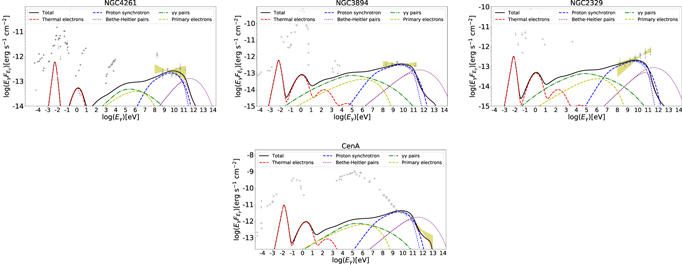
Figure 5. Photon spectra for the "Excellent" objects. The line types are the same as Figure 1. Data points are taken from Tomar et al. (2021) for NGC 4261, Principe et al. (2020) for NGC 3894, Rulten et al. (2020) for NGC 2329, and H.E.S.S. Collaboration et al. (2020) and Abdo et al. (2010) for Cen A. Other data points are taken from the NASA/IPAC Extragalactic Database (NED; http://ned.ipac.caltech.edu).
Download figure:
Standard image High-resolution image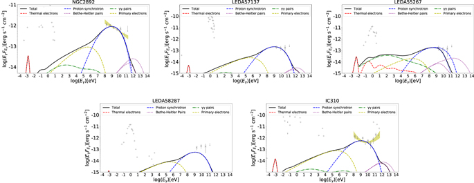
Figure 6. Photon spectra for the "Good" objects. The line types are the same as Figure 1. Data points in GeV gamma rays are taken from Tomar et al. (2021) for NGC 2892, Paliya (2021) for LEDA 57137, LEDA 55267, and LEDA 58287, and Graham et al. (2019) for IC 310. Other data points are taken from NED.
Download figure:
Standard image High-resolution image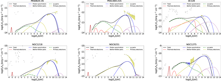
Figure 7. Photon spectra for the "Bad" objects. The line types are the same as Figure 1. Data points are taken from Rulten et al. (2020) for PKS 0625-35, PKS 1304-215, 3C 120, NGC 1218, and NGC 6251, and Tomar et al. (2021) for NGC 1275. Other data points are taken from NED.
Download figure:
Standard image High-resolution imageTable 3. Quantities for the "Excellent" Objects
| Name | Mass (M⊙) | Distance (Mpc) |

| χ2/ν | Q |
|---|---|---|---|---|---|
| NGC 4261 | 4.9 × 10⁸ | 35.1 | 2.2 × 10⁻⁴ | 1.1 | 0.35 |
| NGC 3894 | 5.4 × 10⁸ | 50.1 | 4.5 × 10⁻⁴ | 0.47 | 0.70 |
| NGC 2329 | 4.9 × 10⁸ | 71.1 | 5.7 × 10⁻⁴ | 1.4 | 0.24 |
| Cen A | 5.5 × 10⁷ | 3.8 | 3.9 × 10⁻⁴ | 3.3 | 0.011 |
Note. The references for BH masses and distances are Tomar et al. (2021) for NGC 4261, Mould et al. (2012) and Balasubramaniam et al. (2021) for NGC 3894, Das et al. (2021) and Ellis & O'Sullivan (2006) for NGC 2329, and Harris et al. (2010) and Janssen et al. (2021) for Cen A.
Download table as: ASCIITypeset image
Table 4. Same as Table 3, but for "Good" Objects
| Name | Mass (M⊙) | Distance (Mpc) |

| χ2/ν | Q |
|---|---|---|---|---|---|
| NGC 2892 | 8.4 × 10⁸ | 86.2 | 1.7 × 10⁻³ | 1.53 | 0.19 |
| LEDA 57137 | 1.5 × 10⁹ | 171 | 9.2 × 10⁻⁴ | 0.34 | 0.71 |
| LEDA 55267 | 4.8 × 10⁸ | 327 | 8.9 × 10⁻³ | 1.36 | 0.26 |
| LEDA 58287 | 9.6 × 10⁸ | 185 | 5.7 × 10⁻⁴ | 3.82 | 0.02 |
| IC 310 | 9.0 × 10⁸ | 63 | 6.7 × 10⁻⁴ | 2.74 | 0.018 |
Note. The BH masses are enhanced by a factor of 3 from the values in the references. The references for BH masses and distances are Beifiori et al. (2012) for NGC 2892, Paliya (2021) and NED for LEDA 55267, LEDA 57137, and LEDA 58287, and Schulz et al. (2015) and Ellis & O'Sullivan (2006) for IC 310.
Download table as: ASCIITypeset image
Table 5. Same as Table 3, but for "Bad" Objects
| Name | Mass (M⊙) | Distance (Mpc) |

| χ2/ν | Q |
|---|---|---|---|---|---|
| PKS 0625-35 | 9 × 10⁹ | 243.7 | 2.4 × 10⁻³ | 12 | 1.0 × 10⁻¹¹ |
| PKS 1304-215 | 3 × 10⁹ | 564 | 1.1 × 10⁻² | 13 | 2.5 × 10⁻¹⁰ |
| 3C 120 | 1.89 × 10⁸ | 139 | 1.0 × 10⁻¹ | 65 | 3.0 × 10−42 |
| NGC 1275 | 7.2 × 10⁹ | 70.1 | 5.7 × 10⁻³ | 289 | 0.0 |
| NGC 1218 | 1.65 × 10⁹ | 116 | 1.7 × 10⁻³ | 7.4 | 6.0 × 10⁻⁶ |
| NGC 6251 | 1.84 × 10⁹ | 104.6 | 4.5 × 10⁻⁴ | 4.1 × 10² | 0.0 |
Note. The BH masses are enhanced by a factor of 3 from the values in the references. The references for BH masses and distances are Rani (2019) and Sahakyan et al. (2018) for PKS 0625-35, NED for PKS 1304-215, Hlabathe et al. (2020) for 3C 120, Scharwächter et al. (2013) and Tomar et al. (2021) for NGC 1275, Falcke et al. (2004) for NGC 1218, and Graham (2008) for NGC 6251. For PKS 1304-215, there is no data for BH mass, and we assume the BH mass as 109 M⊙.
Download table as: ASCIITypeset image
Appendix C: Photon Spectra and Resulting Quantities for the Various Radio Galaxies with Another Electron-heating Prescription
We show the photon spectra of the various radio galaxies with the prescription given by Chael et al. (2018). The photon spectra of the "Excellent," "Good," and "Bad" objects are shown in Figure 8, Figure 9, and Figure 10, respectively. We tabulate the resulting quantities in Table 6.

Download figure:
Standard image High-resolution image
Figure 9. Same as Figure 6, but with the electron-heating rate given by Chael et al. (2018). Data points are taken from de Menezes et al. (2020) for NGC 315.
Download figure:
Standard image High-resolution image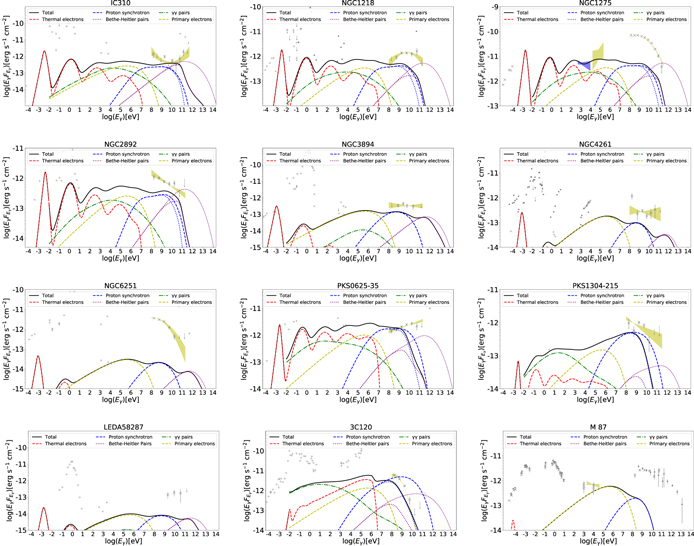
Figure 10. Same as Figure 7, but with the electron-heating rate given by Chael et al. (2018). Data points are taken from MAGIC Collaboration et al. (2020), Prieto et al. (2016), Wong et al. (2017), and Ait Benkhali et al. (2019) for M87.
Download figure:
Standard image High-resolution image
Table 6. Quantities and Classification with the Electron-heating Rate Given by Chael et al. (2018)
| Name |

| χ2/ν | Q | Classification |
|---|---|---|---|---|
| NGC 2329 | 7.3 × 10⁻⁴ | 2.1 | 0.1 | Excellent |
| Cen A | 3.9 × 10⁻⁴ | 2.3 | 0.06 | Excellent |
| LEDA 55267 | 3.8 × 10⁻² | 2.2 | 0.1 | Good |
| LEDA 57137 | 1.9 × 10⁻³ | 0.23 | 0.8 | Good |
| NGC 315 | 1.7 × 10⁻⁴ | 1.6 | 0.14 | Good |
| IC 310 | 8.5 × 10⁻⁴ | 3.2 | 0.0075 | Bad |
| NGC 1218 | 2.0 × 10⁻³ | 23 | 2.9 × 10⁻¹⁹ | Bad |
| NGC 1275 | 1.7 × 10⁻³ | 843 | 0.0 | Bad |
| NGC 2892 | 1.7 × 10⁻³ | 16 | 1.6 × 10⁻¹³ | Bad |
| NGC 3894 | 1.7 × 10⁻⁴ | 7.6 | 4.2 × 10⁻⁵ | Bad |
| NGC 4261 | 1.1 × 10⁻⁴ | 9.1 | 2.5 × 10⁻⁷ | Bad |
| NGC 6251 | 1.3 × 10⁻⁴ | 481 | 0.0 | Bad |
| LEDA 58287 | 2.2 × 10⁻⁴ | 6.4 | 0.0016 | Bad |
| PKS 0625-35 | 4.9 × 10⁻³ | 25 | 1.7 × 10⁻²⁵ | Bad |
| PKS 1304-215 | 1.1 × 10⁻² | 14 | 9.4 × 10⁻¹² | Bad |
| 3C 120 | 1.0 × 10⁻¹ | 97 | 1.1 × 10−62 | Bad |
| M87 | 1.6 × 10⁻⁵ | 44 | 6.1 × 10−148 | Bad |
Download table as: ASCIITypeset image