


Abstract
A transition layer, named the Alfvénic transition layer (or ATL), has been clearly evidenced near the outer boundary of the cusp by experimental observations from the Cluster mission. This layer characterized by a local value of Log MA ∼ 1, where MA is the Alfvén Mach number, allows the bulk flow to transit from super-Alfvénic to sub-Alfvénic from the exterior to the interior side of the outer cusp. The ATL has been observed during northward interplanetary magnetic field orientation, and mainly within the meridian plane. Currently, 3D Particle In Cell (PIC) global simulations of the solar wind–magnetosphere interaction are being performed in order to analyze the cusp region and this layer in detail. Present results stress the following points: (i) the ATL has a 3D structure; (ii) within the meridian plane, the ATL appears as a sublayer within a much more extended slow-mode pattern, and it is almost adjacent and located above the upper edge of the stagnant exterior cusp (SEC); and (iii) the plasma deceleration through the ATL is not uniform in the region located above the cusp. In addition, present preliminary results stress that (a) the spiraled streamlines of ion/electron fluxes converge when approaching the cusp, and their intensity strongly increases; and (b) ion and electron energetic fluxes penetrating the cusp region strongly differ in terms of their penetration depths and are issued from different regions of the magnetosphere/magnetosheath. Our results illustrate the importance of 3D effects used with a PIC simulation approach allowing the analysis of each population simultaneously.
Export citation and abstract BibTeX RIS

Original content from this work may be used under the terms of the Creative Commons Attribution 4.0 licence. Any further distribution of this work must maintain attribution to the author(s) and the title of the work, journal citation and DOI.
1. Introduction
The magnetosphere is the outermost layer of geospace, and the solar wind interaction with the terrestrial magnetosphere is an important issue of the space weather program from Sun to Earth. One of the goals of the space weather program is to analyze the changing environmental conditions from the solar atmosphere to Earth, which is mostly affected by energetic particles from solar wind through the interplanetary space (Wang et al. 2013). The magnetospheric cusp is one of the key regions where the transport of solar wind plasma and energy into the magnetosphere takes place. Then, analyzing the structures and physical processes of the cusp is important for understanding the solar wind–magnetosphere coupling. Low- and mid-altitude cusps have been highly investigated in previous magnetospheric studies (Newell et al. 1989; Yamauchi et al. 1996; Russell 2000), while the high-altitude cusp region was not despite its significant roles. Only later was it studied in detail using the 3D Cluster satellite fleet (Lavraud et al. 2002; Nykyri et al. 2003; Lavraud et al. 2004a, 2004b; Cargill et al. 2004; Lavraud et al. 2005). One striking feature is the evidence of a transition layer (in terms of Alfvén Mach number) located above the high-altitude cusp and on the boundary of the magnetosheath. More precisely, this Alfvénic transition layer (ATL) has a narrow width and is characterized by a rapid variation of the flow Alfvén Mach number MA from a super-Alfvénic regime in the magnetosheath region to a sub-Alfvénic regime when penetrating the upper edge of the stagnant exterior cusp (SEC) as shown by Lavraud et al. (2005), MA = Vflow/VA, where local Vflow is the plasma bulk velocity and local VA is defined by VA = B/(ρμo)1/2, in which B is the magnetic field value, ρ is the mass density of particles, and μo is the permeability of the free space. A detailed analysis of this layer may provide important information for understanding flow variations and particle precipitations in the upper edge of the high-altitude cusp. Cai et al. (2015) have performed 3D Particle In Cell (PIC) simulations of the global solar wind–terrestrial magnetosphere interaction under northward interplanetary magnetic field (IMF) conditions and have focused their attention on the cusp region. They have retrieved quite good agreement between experimental observations and the different frontiers of the cusp, including in particular the SEC region and the ATL adjacent to the upper edge of the cusp.
The present study is an extension of the previous work by Cai et al. (2015) and is mainly focused on the ATL features for a northward IMF case, in order to clarify the following questions: (i) Can the ATL be extended outside the cusp region ? (ii) Since previous experimental and simulation analyses mentioned above have been performed within the meridian plane only, does the ATL persist out of the meridian plane? (iii) If yes, what are their characteristics when moving dawnward/duskward from this plane (in terms of spatial scale and location)? (iv) What is the link between the SEC region identified in previous experimental data (Lavraud et al. 2002, 2004b, 2005) and simulation results (Cai et al. 2015) and the ATL? (v) How are the 3D features of the ion and electron fluxes penetrating the cusp, and what regions outside the cusp are these most energetic fluxes originating from?
The outline of this paper is summarized as follows. The 3D simulation model and physical parameters are briefly described in Section 2. Section 3 gathers the main results of the cusp region and of the extended region of the ATL obtained for a northward IMF. Section 4 presents the relationship between the SEC region, the ATL, and the characteristics of particle precipitation in the cusp; preliminary results of this precipitation are analyzed based on 3D structures and intensity of electron/ion fluxes separately. Discussion and conclusions are summarized in Section 5.
2. Three-dimensional Global PIC Simulation Model
In the present simulation, we use the same initial conditions to form the magnetosphere and the same radiating boundary conditions and charge-conserving formulae as those used in our previous works (Cai et al. 2006; Cai & Buneman 1992). Three-dimensional global interactions between the solar wind and the magnetosphere are performed herein, but we mainly focus our attention on the cusp region, where 3D and kinetic effects play an important role (particle entries). Due to computational constraints, the spatial grid is not fine enough to include most kinetic plasma instabilities. However, the interaction between the macroscopic electric and magnetic fields and the electrons/ions and their related accelerations are included self-consistently.
The number of particles within the simulation Debye sphere is about 30, and some particle collisional effects may be expected (Birdsall & Langdon 1985). Thus, a smoothing technique is applied to reduce the expected noise (Buneman et al. 1980, 1992; Buneman 1993). An ionosphere model is not implemented, and particles entering the region corresponding to the ionosphere at a distance less than 10 Δ (i.e., at distance lower than 2 Re) are automatically removed from the simulation, where Δ is the grid size. The simulation box in x, y, and z is limited so that the 3D nearby tail region is fully included, but the far magnetotail region (x > 38 Re) is excluded from our analysis, even if partially included in our numerical simulations. The Alfvén Mach number of the solar wind is relatively low at about MA,SW = 2.6.
The simulation domain is identical to that already used in previous work (Cai et al. 2015). In short, a 3D PIC simulation is performed with a space grid Δ = 0.2 Re and a time step Δt = 1ωpeΔt = 0.125 (ωpe is the electron plasma frequency), where the grid size is Δ =Δx = Δy = Δz . Initially, the sizes of the simulation box illustrated in Figure 1(a) are (365 Δ, 275 Δ, 275 Δ), and we use a uniform particle density of ne = ni = 8 pairs per cell throughout the simulation box, i.e., about a total of 227 × 106 electron–ion pairs. The time sequence of the IMF application is shown in Figure 1(b). At time t = 0, the dipole (representing the dipolar terrestrial magnetic field) is located in the simulation box at (160 Δ, 137.5 Δ, 137.5 Δ), and a solar wind bulk velocity VSW = 2.6 VA is continuously applied within the time range 0 < t < 3000 along the x-axis without any IMF (the time is expressed in terms of Δt units). The injected solar wind density has also n = 8 electron–ion pairs per cell, and the mass ratio is M i /me = 16. A northward IMF is progressively applied over the time range 3000 < t < 3150 and remains constant after t = 3150 until the end of the simulation (t = 9000), which is defined as when the solar wind particles carrying the IMF have had enough time to cross the simulation box several times (3.2 times for the present simulations). Table 1 includes the definition of normalized solar wind physical quantities and plasma parameter values used in the present simulation separately for electrons and ions; hereinafter, for convenience, we will omit the tilde notation "∼" used for normalized quantities.
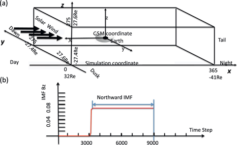
Figure 1. (a) Simulation reference frame (GSM). The terrestrial center is located at (160 Δ, 137.5 Δ, 137.5 Δ) or equivalently (32 Re, 27.4 Re, 27.4 Re). In the simulation coordinates, the left front corner is the origin; the unit is the grid size. (b) Time history of the applied northward IMF. The unit is the time of the simulation (from Cai et al. 2015).
Download figure:
Standard image High-resolution imageTable 1. Parameter Normalization and Plasma Values of the Solar Wind Defined for Electrons and Ions
| Parameter | Normalization | Electron | Ion |
|---|---|---|---|
| Thermal velocity |

| 0.125 | 0.0625 |
| Debye length |

| 1.4 | 2.8 |
| Larmor gyroradius |

| 1.56 | 12.6 |
| Gyrofrequency |

| 0.08 | 0.005 |
| Inertia length |

| 4 | 16 |
| Plasma frequency |
| 0.125 | 0.031 |
| Gyroperiod |

| 78.5 | 1256 |
| Temperature |
| 0.008 | 0.032 |
Download table as: ASCIITypeset image
As in Cai et al. (2015), let us remind that normalized parameters can be converted to physical values based on typical real solar wind and magnetospheric plasma conditions. The minimum distance from Earth's center to the dayside magnetopause (MP) Rmp is about 50 grid sizes. All the physical values are scaled by Rmp and the solar wind velocity Vsw. If one assumes Rmp = 64,000 km (i.e., 10 Re, where Re = 6400 km is Earth's radius), the solar wind velocity Vsw = 300–600 km s−1; here 400 km s−1 is chosen as a typical value, one grid size Δ is about 1280 km (=0.2 Re), and 1000 simulation time steps represent ∼7–14 minutes, or about ∼0.64 s per simulation time step. The electron Debye length equals ∼ 1792 km, and the electron thermal velocity equals ∼250 km s−1 (which are rather not realistic but represent a compromise because of computational constraints). These initial conditions indicate that the kinetic effects of space charge and particle acceleration (for both electrons and ions) are included but most plasma instabilities are excluded. For example, the upstream ion gyroradius is relatively large (ρci = 12.5Δ = 2.5 Re from Table 1) as compared to the physical situation (ρci (H+) = 500–2000 km = 0.078–0.31 Re). The gyroradius used here is obtained from a spatial average within the cusp, including the so-called SEC (defined in Figure 3(a)).
3. Main Results Obtained for Northward IMF
The global magnetic field configuration is shown in Figure 2(a) at a late time of the simulation (t = 9000) for a northward IMF. It is similar to that of Figure 2 of Cai et al. (2015), where all simulation details may be found. An enlarged view of the magnetic field B in the cusp region is shown within the meridian plane x–z in Figure 2(b): the red trapezoid indicates the location of SEC; the white rectangle indicates a possible reconnection region where B amplitude is very weak. The detailed analysis of Cai et al. (2015) has allowed us to recover the main features of the cusp region (strong B field amplitude and weak plasma density), which are illustrated in Figure 3(a). In short, this region can be relatively well defined by the spatial profiles of the B-gradient and of the density from low to high altitudes. Based on statistical observations from Cluster satellites (Lavraud et al. 2004a, 2005), a typical SEC or diamagnetic cusp region may be defined. For a northward IMF, the SEC region has four edges, namely, poleward, upper, lower, and equatorial edges (Figure 3), and has been analyzed in the numerical simulations of Cai et al. (2015). Figure 3(b) shows the electron density amplitude issued from present 3D PIC simulations that allows us to identify clearly the cusp region, where the electron density is very high (red "tooth shape" region); this plot will be used as a reference to identify the cusp. Moreover, it also shows the SEC region, where the electron density decreases (blue trapezoid) when moving from the magnetosheath (high altitude) to the cusp (middle altitude).
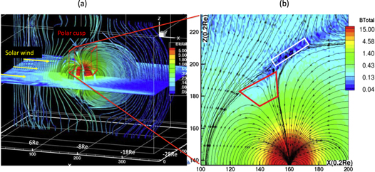
Figure 2. (a) 3D magnetic field streamlines for the terrestrial magnetosphere under northward IMF conditions issued from 3D PIC simulations at a late time t = 9000; the x-axis corresponds to the line Sun–Earth. (b) Enlarged view of the cusp region identified within the cube shown in panel (a) showing colored mapping (B amplitude) and field lines of the total magnetic field in the meridian plane X–Z (used as a reference plane in the next figures).
Download figure:
Standard image High-resolution image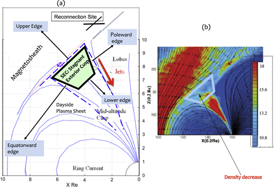
Figure 3. (a) Schematic sketch of the cusp region, its surrounding boundaries, and main areas in the meridian plane (adapted from Lavraud et al. 2004). The trapezoid indicates the location of the SEC, where the perpendicular convection flow (VperpX) and the density are very weak. (b) Colored plot of the electron density issued from present 3D PIC simulations within the (x, z) meridian plane defined at y = 137.5 Δ; magnetic field lines are reported in the 2D plane.
Download figure:
Standard image High-resolution imageOne striking feature appears at/near the upper edge that is characterized by a transition layer (ATL) where the plasma flow varies from the super- to sub-Alfvénic regime when passing from the magnetosheath region to the SEC region. To the knowledge of the authors, this ATL has been observed for the first time experimentally by Lavraud et al. (2005) and is evidenced in 3D PIC simulations by Cai et al. (2015) for the northward IMF and in the meridian plane only.
3.1. Main Morphological Features of the ATL inside the Meridian Plane
Following the previous works by Lavraud et al. (2005) and Cai et al. (2015), one way to evidence the precise location of the ATL consists in plotting a map of Log MA within the (x–z) meridian plane passing through Earth's location. The results for a northward IMF are shown in Figure 4, which shows a good agreement between simulation results (panel (a)) and experimental measurements (panel (b)). A more detailed analysis of the present simulation allows us to extend the observations as follows:
- (i)Within the meridian plane, the ATL not only is limited to the upper edge of the cusp but also may be identified even far outside the cusp region. It extends both toward the equatorial plane to the subsolar point of the MP and toward the nightside as illustrated in panel (a).
- (ii)For reference, the location of the MP where the IMF is piling up against the magnetosphere is represented by red dashed lines in Figure 4(a), which clearly shows that the correspondence of the ATL and the MP is not straightforward everywhere. Both frontiers do have the same location when moving from the cusp region to the nightside of the magnetosphere. In contrast, these strongly differ one from each other on the dayside from the subsolar point to the cusp region. At/around the subsolar point, the ATL is located much upstream from the MP, which means that the deceleration of the plasma flows in the magnetosheath (downstream of the bow shock not represented herein) is quite efficient, and the flow regime becomes sub-Alfvénic much before reaching the MP itself. However, the situation changes when moving above the subsolar region in the direction of the cusp, where the ATL width increases but its location approaches the MP. When approaching the cusp itself, the ATL width strongly decreases (as illustrated by the size of dark dashed trapezoids in Figure 4(a)) to become very thin, and ATL and MP locations become mixed.
- (iii)More local spatial information may be obtained on the ATL by performing measurements of its thickness along different orientations of radial slicing lines. The global plot including all lines within the x–z meridian plane is shown in Figure 5(a), while three enlarged views of the same meridian plane are shown, respectively, in Figures 5(b), (c), and (d). The different orientations of the slicing lines have different identification numberings extending from index #1 (at the subsolar point) to index #91 (in the tailward lobe of the cusp). In order to measure the ATL width along the different slices, we have reported the values Log MA = 0.2, 0.0, and −0.2, which are shown by white, blue, and black circles, respectively, and which are used as reference values; the ATL width (ΔATL) is determined by the distance between white and black circles. At a first glance, Figure 5(a) shows clearly that this width ΔATL is strongly varying according to the slicing direction in particular within the cusp region (panel (c)) and when moving outside the cusp region in the direction of the subsolar point (panel (b)). In order to get more precise measurements, the ATL width has been measured along each indexed line and is reported in Figure 6. The strong variation of ΔATL versus the line index leads to defining four characteristic slicing directions used as references to define some angular sectors: LA (#22), L1 (#36), LB (#50), and L2 (#63). If one considers the subsolar line along the Sun–Earth axis as the 0° reference direction, the corresponding line direction is LA (29°), L1 (48°), LB (66°), and L2 (84°), respectively. These features indicate that the braking of the plasma flow is not uniform through the whole ATL (i.e., takes place over strongly varying spatial range) and depends on the angular direction of the indexed line. These ATL features will be analyzed versus the precise location of the cusp and of the SEC in Section 4.2.
- (iv)Let us focus on line L2. Amplitude profiles of the ion density, of the magnetic field, and of Log MA have been measured versus x-axis (i.e., more precisely along line L2 projected along the x-axis) and are reported in Figure 7. Moreover, the values Log MA = −0.2 and 0.2 are indicated by arrows (bottom panel), so that one can precisely identify the ATL location (pink vertical bar); the value MA = 1 (i.e., Log MA = 0) is indicated by a vertical red dashed line. Main regions are identified by different colored bars to clarify the discussion of the variation of the different quantities along the x-axis.

Figure 4. (a) Color-coded mapping of Log MA within the meridian plane defined at y = 137.5 Δ for a northward IMF at late time t = 9000, where MA is the Alfvén Mach number, observed in present PIC simulations; the possible "X" reconnection region where B is very weak as identified in Figure 2(b) is reported by a dark thick cross in panel (a); the small trapezoids (black dashed lines) are used here in order to indicate the changing thickness of the ATL region; the dashed red line indicates the location of the MP. (b) Corresponding results of Log MA measured from Cluster data (issued from Figure 5 of Lavraud et al. 2005); the "outer boundary" illustrates the location of the ATL. The B field lines (in white and black) are reported in panels (a) and (b), respectively.
Download figure:
Standard image High-resolution image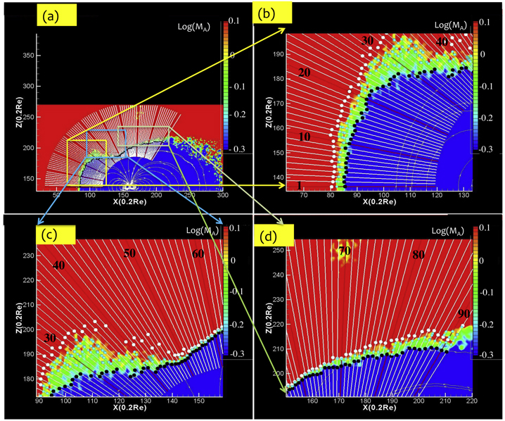
Figure 5. (a) Plot of Log MA amplitude measured for northward IMF within the x–z meridian plane defined at y = 137.5 Δ. White curved streamlines show the magnetic field lines, and the oblique lines represent the radial indexed lines that are extended from #1 (in the subsolar point) to #91 (in the tailward lobe). White, blue, and black circles show the locations corresponding to values Log MA = 0.2, 0.0, and −0.2, respectively. Panels (b), (c), and (d) are enlarged views of panel (a) in the areas defined by three colored rectangles in panel (a).
Download figure:
Standard image High-resolution image
Figure 6. (a) Thickness ΔATL of ATL measured along each radial indexed line between points where Log MA = −0.2 and Log MA = 0.2 defined in Figure 5 for the purely northward IMF case at a late time t = 9000 of the simulation. The x-axis corresponds to the index (i.e., the direction) of the radial lines varying from #1 (subsolar point) to #91 (in the tailward lobe) defined in panel (b). (b) Plot of the Log MA with superimposed white radial indexed lines defined from #1 to #91 as in Figure 5. Red radial lines indicate each new tens of line index value. The characteristic radial slicings LA, LB, L1, and L2 defined in panel (a) are reported.
Download figure:
Standard image High-resolution image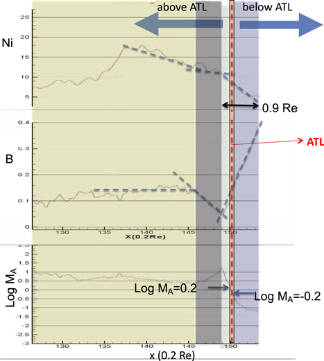
Figure 7. Amplitude profiles of (a) the ion density, (b) the total magnetic field, and of (c) the Log MA value measured along the L2 radial line defined in Figure 6 within the meridian plane. Measurements are performed vs. distance x, i.e., vs. the projection of the L2 radial line on the x-axis (not to be confused with the distance defined along each radial line in Figure 6). Different x ranges are identified by four colored bars. The ATL is identified by a narrow red bar centered around the value Log MA = 0 shown by a red vertical dashed line. Dashed light-blue lines correspond to locally averaged values of the quantities.
Download figure:
Standard image High-resolution imageThe following features are observed: two main areas may be defined below and above the ATL location, respectively. For reference, increasing x-value corresponds to approaching Earth. As x increases in the region above the ATL within the yellow bar, the locally averaged values (dashed blue lines) show that the density Ni decreases while B field amplitude is almost constant. When approaching the ATL, both Ni and B decrease (gray bar). However, very near the ATL, Ni still decreases while B increases strongly (green bar), which characterizes a slow-mode pattern. The strong increase of B contributes to the braking of the magnetosheath flow through the ATL and corresponds exactly to the important decrease of Log MA (green and blue bars) until it reaches a minimum value farther in the region below the ATL (Log MA = −1.1 in the blue bar). Let us note that the maximum Log MA value corresponds to the location of the minimum B field. However, the location of the ATL does not correspond to that of the minimum B field, which is not far from the X-point location (reconnection region in Figure 4). Then, the ATL appears as a sublayer (with a narrow width ΔATL = 0.1 Re in Figure 7 within a much more extended slow-mode pattern (total width of green and blue bars covers 0.9 Re). It is important to precise that the present value ΔATL = 0.1 Re (measured along the L2 line projected on x-axis) should not be confused with the value found in Figure 6 (ΔATL = 0.5 Re) measured directly along the L2 line. These features remind the ones defining the presence of the plasma depletion layer (PDL). The relationship with the PDL requires a further analysis, which is under investigation.
3.2. Main Morphological Features of the ATL outside the Meridian Plane
(i) The width of the ATL is very thin around the upper edge of the cusp region. Present results show that the ATL not only is identified within the meridian plane but also extends outside this plane. This has been evidenced by performing an animation of the Log MA plot within a plane (x–z), i.e., parallel to the meridian plane moving along the y-axis from the duskside to the dawnside. Within each plane y-location, the ATL width is measured between the values Log MA = (0.2, −0.2) along the same indexed line used as a reference (L = 57), i.e., between LB and L2 identified in Figure 6. This reference line has been chosen where the ATL width is very thin within the meridian plane, so that one can easily follow its variation when moving on each side of this plane. Results are illustrated in Figure 8, which shows that the ATL width ΔATL decreases within the dusk region when approaching the meridian plane located at y = 137.5Δ until reaching a minimum ΔATL = 0.75 Re. In contrast, ΔATL strongly increases when moving farther from the meridian plane within the dawn region. The variation is not symmetrical between dusk and dawn regions. In addition, the averaged width values measured within dusk and dawn regions are ΔATL = 2.06 Re and 2.23 Re, respectively. The reasons for these dusk–dawn differences are still under active investigation.

Figure 8. Measurements of the ATL width ΔATL within a plane (x–z) parallel to the meridian plane and moving along the y-axis from the dusk to the meridian plane (panel (a)) and from the meridian plane to the dawnside (panel (b)). The horizontal axis of the plot corresponds to the y-location of the moving plane (for reference the meridian plane is located at y = 137.5 Δ). For each y-location, the ATL width is measured between the values (−0.2, 0.2) of Log MA along a fixed radial indexed line #57 defined in Figure 5 and used as a reference herein. This line location is reported in the (x–z) planes defined at y = 110 Δ (dusk region in panel (c)) and 175 Δ (dawn region in panel (d)) in the bottom part of the figure. The averaged values of ΔATL in dawn and dusk regions are ΔATL = 2.06 Re and 2.23 Re, respectively.
Download figure:
Standard image High-resolution image(ii) A more complete analysis of the asymmetric features of the ATL between dawnside and duskside can be performed by identifying the location LATL of the ATL where Log(Ma) = 0 measured along the same indexed line L = 57 within a given (x–z) plane moving along the y-axis as in the previous subsection. The ATL location versus Y is reported in Figure 9; line L = 57 is illustrated by the white line in plot (c) defined at y = 138 Δ. Far in the duskside (dawnside) from the meridian plane, i.e., as Y is weak (high) in panel (a) (panel (b)), the ATL location is very near the planet (i.e., LATL is weak). However, when approaching the meridian plane, its location increases until LATL reaches a maximal asymptotic value (LATL = 10.5 Re and 11.5 Re) indicated by a dashed red line in panels (a) and (b) within dusk and dawn regions, respectively. Then, the variation ΔLATL of the ATL location looks symmetric on each side of the meridian plane, but the spatial scale within which its location varies between dawnside and duskside is slightly asymmetric (ΔLATL = 7.2–10.5 Re and 8.0–11.5 Re in panels (a) and (b), respectively).
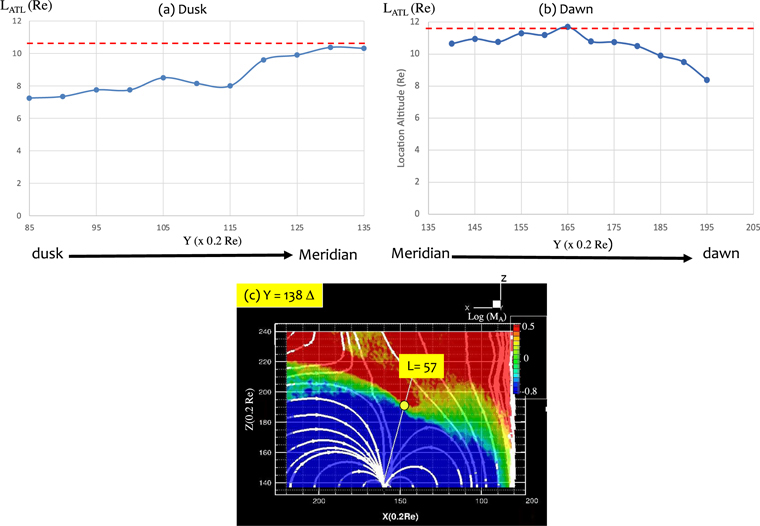
Figure 9. Location LATL of the ATL measured along the same reference radial line L = 57 defined within a given (x–z) plane parallel to the meridian plane and moving along the y -axis. Results vs. y -location are reported in panels (a) and (b), respectively, from the dusk region to the meridian plane and from the meridian plane to the dawn region. The ATL location is defined where Log MA = 0. Panel (c) illustrates the location of the radial indexed line L = 57 as the moving (x–z) plane is located at y = 138 Δ; the ATL location is illustrated by a thick white circle along this indexed line.
Download figure:
Standard image High-resolution imageIn summary, present results evidence that the ATL has a 3D extension (i.e., within and outside the meridian plane) and its features present some asymmetry between dusk and dawn sides. This asymmetry is noticeable in its width ΔATL and its spatial location LATL outside the meridian plane. In addition, the width ΔATL drastically varies within a transition region from dayside to the cusp as defined between LA and LB in Figure 6(a), when measured within the meridian plane. Such 2D and 3D mappings are helpful for collecting more precise information to identify structures of the cusp where particle precipitation is expected to be the strongest. This point is addressed in the next section.
4. Mappings of the SEC within the Meridian Plane, the ATL, and 3D Ion/Electron Fluxes
4.1. Main Features of the SEC
A deeper analysis may be performed to define more precisely the locations of the SEC, in particular, how L1, LB, and L2 lines (Figure 6) are located with respect to the different edges of the SEC defined at high altitude of the cusp (as illustrated in Figure 3(a)). As a reminder, the SEC has four edges more precisely defined as follows (Cai et al. 2015):
- (i)The upper edge where the parallel ion bulk flow changes from upward (V// > 0, in the magnetosheath, i.e., above the SEC) with a large tailward convection to downward (V// < 0, inside the SEC) associated with a very weak almost "stagnant" tailward convection. Let us remind that upward (V// > 0) and downward (V// < 0) indicate, respectively, the direction opposite to and the same as the local magnetic field.
- (ii)The poleward edge is characterized by an inversion of the parallel ion flux from V// > 0 (strong and upward outside the SEC region) to V// < 0 (weak and downward inside the SEC region with sunward convection).
- (iii)Commonly, the equatorial edge only represents the link between the cusp region and the dayside plasma sheet. Cai et al. (2015) have shown that poleward and equatorial edges may also be defined more precisely as frontiers where the electron kinetic energy is quite high (inside the SEC) and very low (outside the SEC).
- (iv)No precise definition has been commonly proposed yet for the lower edge of the SEC. However, present results (Figure 3(b)) stress that the electron density is varying from very low (inside the SEC) to high values (at altitudes below the lower edge and above its upper edge); similar variation is observed for ion density (Figure 8(c) of Cai et al. 2015).
The SEC appears as a particular transition region where kinetic energy of each population is high outside but weak inside; it is also identified as a diamagnetic region where density is low but magnetic field is high. These previous statements are analyzed more carefully in Sections 4.2 and 4.3.
4.2. SEC and ATL
Cai et al. (2015) have evidenced that ions and electrons dynamics differ within the cusp region. The authors stressed that the region of enhanced ion density extends more deeply into the cusp region than the area where high-energy ions are found. This suggests that many ions penetrate into the deep cusp but are decelerated. This suggestion may be verified by plotting an enlarged view of Log MA, of the electron density, of electron kinetic energy, and of ion kinetic energy in the vicinity of and within the cusp region as shown in Figure 10, within the meridian plane located at y = 137.5 Δ. The "funnel-shaped" cusp is characterized by a long electron penetration depth (distance d1 = 8 Re) and its large angular range (distance d2 = 8 Re) in Figure 10(b) of the electron density used as a reference plot to identify the cusp. For reference, the location of the SEC (trapezoid frame) has been reported in all panels, which shows that the SEC is well located within the subsonic flow region (blue part in Figure 10(a)). The comparison of plots confirms that electrons (and ions) succeed in penetrating deeply but are decelerated as the plasma flow gets a sub-Alfvénic regime through the ATL (almost adjacent to the upper edge of the SEC). In addition, the locations of reference lines L1, LB, and L2 (defined in Figure 6(a)) have also been reported in order to clarify the relationship between the shape and the location of the cusp (Figure 10(b)) and the features of the ATL (in particular the angular variation of its width shown in Figure 6(a)). Let us note that the equatorial edge of the SEC is near line L1, while line LB is near the poleward edge of the SEC (as defined in Figure 3(a)). The large variation of the ATL width (Section 3) brings additional information as follows:
- (i)Figure 10(a) shows that the SEC is mainly located within the range between lines L1 and LB, where the ATL width is large. More precisely, the plasma deceleration takes place progressively, i.e., over a large spatial ATL width around line L1; however, this spatial range (i.e., ATL width) decreases until reaching a minimum value when approaching line LB, i.e., the poleward edge of the SEC. In other words, the plasma deceleration around the upper edge of the SEC is not spatially uniform. This is illustrated by Figure 10(c), which shows the corresponding electron kinetic energy within the same scales as Figures 10(a) and 10(b). Two parts may be identified within the SEC in panel (c): one is characterized by low-energy electrons within the part of the SEC around line L1 (i.e., green area within the SEC), while the other one corresponds to electrons that still have some high energy within the part of the SEC approaching LB (i.e., red area within the SEC). The first and second areas are, respectively, located where the ATL width is still large and becomes quite narrow. The evidence of this strong inhomogeneity in the electron kinetic energy within the SEC itself may be due to 3D spiraling effects that particles suffer when penetrating the cusp region itself. This point is discussed in Section 4.3.
- (ii)While the electron and ion (not shown herein) density plots are very similar, the kinetic energy differs noticeably between electrons (Figure 10(c)) and ions (Figure 10(d)) within the cusp region (area between L1 and LB) as follows: (a) the ion kinetic energy is weak almost everywhere within the SEC region, in contrast with electrons; (b) energetic electrons succeed in penetrating much more deeply into the cusp (red area below the SEC) than ions, and indeed the corresponding electron kinetic energy plot shows a "funnel shape" (red region) similar to the electron density cusp in contrast with ion kinetic energy; (c) some energetic ions still persist just below the SEC but are limited to a small area. All these results suggest that ions are more easily decelerated through the ATL (above/around the upper edge of the SEC) when penetrating the cusp than electrons.
- (iii)Figure 10(b) shows clearly that the cusp region where the density of electrons is high (i.e., particles accumulate below the SEC) and the SEC itself are mainly located between lines L1 and LB. Moreover, the angular range between LB and L2 includes the reconnection "X" region, i.e., is located outside the cusp region as shown in the present meridian plane. Energetic electrons are continuously evidenced between the "X" region, the area of the SEC located around LB (as mentioned above), and the area below the SEC itself; this is in contrast with ions where disruption of energetic ions is observed within the SEC itself. But a certain attention must be paid, since Figure 10 (as well as Figure 6) is restricted to the meridian plane. Their 3D distributions outside the meridian plane are missing. The possible significance of 3D effects is discussed in Section 4.3.
- (iv)Then, the cusp region (defined within L1–LB) appears as an angular transition area defined between two regions: one is characterized by a thin ATL width (LB–L2 range, and above L2); the other is characterized by a thick ATL width that decreases when approaching the dayside (LA–L1 range) as illustrated in Figure 6(a).
- (v)A deeper investigation has been performed in order to analyze electron and ion energy outside the meridian plane. For this purpose, an animation of the kinetic energy plot measured within the (X–Z) plane parallel to the meridian plane and moving along the y-axis has been performed within the dusk region–meridian plane (80 Δ < y < 137.5 Δ) and the meridian plane–dawn region (137.5 Δ < y < 195 Δ), respectively. This procedure applied separately to electron and ion kinetic energy stresses the following results: (a) the energetic electrons are still well observed within the very deep cusp region (the deepest location is reached for y = 138 Δ, i.e., very near the meridian plane); (b) in contrast, energetic ions are never observed so deeply within the cusp; however, these reach a deep region outside the meridian plane (for y = 140 Δ, which is slightly in the dusk region). These different behaviors between ions and electrons may be associated with different 3D ion and electron motions, respectively; in addition, the impact of present numerical conditions (low mass ratio and grid size scaling) must be analyzed. These open questions are still under investigation.
- (vi)The animation procedure used above allows us to get an estimate of the opening angle of the cusp outside the meridian plane. One uses the location of energetic particles as a reference signature of the cusp within the plane moving from the meridian plane (to dusk and dawn regions); the electron signature is relatively precise since it follows well the "funnel" shape of the cusp (Figure 10(c)); it is similar to that of electron density (Figure 10(b)). In contrast, a similar procedure has been tentatively applied to ion signature, but it appears to be much less precise and the source of uncertainties in the measurements. Then, we choose to focus mainly on energetic electrons results (https://www.youtube.com/watch?v=4O3bqd14v5g). In the dawn region, energetic electrons are not observed any more for y = 147 Δ at location (x = 145 Δ, z = 170 Δ), which leads to an opening angle value α = 28
 6 from the meridian plane. In the dusk region, the energetic electron signature disappears for y = 122Δ at location (x = 150 Δ, z = 178 Δ), which leads to an opening angle value Δ = 278 from the meridian plane. Then, it is clear that (a) the cusp axis location is mainly centered within the meridian plane (the α values are almost symmetrical with 286 and 2708) and (b) the resulting total opening angle of the cusp is 5568. This value is in a good agreement with the corresponding value deduced from the ion density (542) found by applying the same procedure. These values are preliminary estimates of the cusp angle at the present stage of the study.

Figure 10. 2D colored mappings (a) of Log MA, (b) of the electron density, (c) of the electron kinetic energy, and (d) of the ion kinetic energy. All plots are defined within the meridian plane (x–z) located at y = 137.5 Δ. In panel (b), the penetration depth and the opening range of the cusp region can be estimated by measuring, respectively, the distance d1 (along the cusp axis) and the distance d2. In all plots, the trapezoid represents the location of the SEC (defined from Figures 2(b) and 3(b)), and angular locations of lines L1 (48°), LB (66°), and L2 (84°) of Figure 6 have also been reported.
Download figure:
Standard image High-resolution imageSome differences ((i) within the SEC itself, (ii) different penetration depths within the cusp) have been observed between ions and electrons that are out of scope of the present paper and will be analyzed in a later study. However, these differences raise the following question: Is it possible to determine which regions outside the cusp these "energetic" populations come from, respectively, for ions and electrons? This question is addressed in Section 4.3.
4.3. Ion and Electron Fluxes
Present 3D PIC simulations allow us to analyze separately ions and electrons in order to determine their origin before penetrating the cusp. This question can be addressed by plotting the 3D streamlines of both ion and electron fluxes outside and within the cusp region. Results for ions are shown in Figure 11 combining 3D flux streamlines and isocolors of total ion flux Ji,tot in 2D planes used as references; moreover, the varying color along each streamline indicates the local intensity of the associated flux. Figure 11(a) stresses the following results:
- (i)When approaching the cusp, large-scale spiraling ion fluxes converge and concentrate spatially near the entrance of the "funnel-shaped" cusp indicated "visually" by white dotted lines (shown in the middle of the white square).
- (ii)Most streamlines of high-energy ion fluxes (in red) are issued from the subsolar region and slightly from the dawn region (i.e., are related directly to the magnetosheath); no apparent direct link appears with the reconnection region. In contrast, streamlines of lower ion fluxes may be related to the reconnection.
- (iii)Deeper investigations may be performed on the origin of the most energetic ions. For this purpose, enlarged 3D views have been performed and are reported in Figures 11(b) and 11(c) with different view angles. The view angle of Figure 11(b) is similar to that of Figure 11(a), while the 3D plot in Figure 11(c) corresponds to a projection on the (x–y) equatorial plane (i.e., z-axis is perpendicular to the figure). This last view allows us to identify more clearly the dawn and dusk regions separately; it is important to precise that the red vertical line in the middle of Figure 11(c) represents the (x–z) plane as its "slice." Because of their spiraling trajectories near the polar region, the complexity of ion flux streamlines may be analyzed by tracking these back from letters A to C in Figure 11(c). Starting from the final ion penetration within the cusp (letter A), it is clear that the most energetic ion fluxes come from the dusk region (letter B), after approaching the cusp from the dawn region (letter C). Then, by combining Figures 11(b) and (c), one can conclude that ions issued from the subsolar region and around the dawn region contribute strongly to the formation and precipitation of energetic ions. A better analysis may be established by performing a similar 3D plot projected within the (x–z) plane as shown in Figure 11(d) (y-axis is now perpendicular to the figure). This representation is a 3D projection viewed from the duskside and differs from the meridian (x–z) plane defined as a slicing within the 3D plot at y = 137.5 Δ. However, this representation "approaches" the meridian plane and includes simultaneously "projected" 3D ion flux streamlines. Then, we have reported the angular locations of L1 (48°), LB (66°), and L2 (84°) lines identified from Figure 6(a) and the location of the SEC as deduced from Figure 10. Present results clearly confirm that (a) ions accumulate and precipitate between lines L1 ad LB, which corresponds to the angular range of the cusp (Section 4.2); (b) the size of the ion flux spirals is quite large at the entrance of the cusp (which makes the ion trajectories very elongated) and decreases as ions penetrate more deeply within the cusp; and (c) the high intensity of the ion fluxes (red streamlines) appears to be located just below the SEC. In fact, a progressive rotation from panel (a) to panel (c) allows us to state that these high-intensity fluxes correspond to large spiraling ion flux streamlines that do not pass directly through the SEC region but are issued from the subsolar/dawn region (as mentioned above) (see https://drive.google.com/file/d/12c6VNEkEuhcX5dvnYskW8iyuSf1kbQBd/view?usp=sharing). This stresses the importance of 3D effects not accessible by considering only the meridian plane, and that the presence of high-energy ions below the SEC (Section 4.2) is only the signature of large spiraling ion flux streamlines cut by the meridian plane (Figure 10(d)). With deeper penetration, the spiral size and the local intensity of ion fluxes decrease (Figure 11(d)), and no high-energy ions can be evidenced (Figure 10(d)).
- (iv)The situation strongly differs for electrons. As expected, the electron flux streamlines exhibit a much smaller spiraling structure owing to the light electron mass when penetrating into the cusp (Figure 12(a)). The main features are as follows: (a) the spiral size of the electron flux streamlines is very small, and correspondingly the ion flux streamlines look elongated (Figure 11(a)); (b) the backtracking procedure of the streamlines similar to that used for ions is now applied to electrons and allows us to show that high-energy electron fluxes are not related to streamlines only issued from the subsolar and dawn regions (in contrast with ion fluxes); (c) the enlarged 3D view of Figure 12(b) (view angle similar to that of Figure 11(b) for ions) shows that, in contrast to ions, the electron flux intensity is very strong (red part of the spiral within the white rectangle of Figure 12(a)) around the upper edge of the cusp; and (d) a 3D view projected onto the (x, y) equatorial plane shown in Figure 12(c) (view angle similar to that of Figure 11(c)) allows us to separate more clearly dawn and dusk regions. A progressive rotation from panel (a) to panel (c) (see https://drive.google.com/file/d/1Y7vSXJZO6gkwg4fuEvGPDtK8i1IuQexJ/view?usp=sharing) shows that energetic electron fluxes (red part of the streamlines) are mainly issued from two different regions: one corresponds to very high altitude from the dawn flank region (letter "A" in Figure 12(c))/subsolar region (letter B in Figure 12(c)); the other corresponds to lower altitude from the dusk flank region (letter C in Figure 12(c)).

Figure 11. 3D view of ion flux streamlines. (a) 2D Isosurfaces of the total ion flux are represented within two different planes (namely, x–y (equatorial) and x–z (meridian) planes) with a perspective view around the cusp region. Partial transparency is applied to the different planes in order to follow continuously the 3D ion flux streamlines that are superimposed; along each streamline, the color changes and indicates the local intensity of the ion flux. The solar wind is flowing along the x -axis (blue arrows). (b) Enlarged view of the cusp region within the white rectangle of panel (a). The white dotted straight lines in panels (a) and (b) indicate the frontiers of the "funnel-shaped" cusp. The 3D ion flux streamlines converge into the cusp where the flux intensity is maximum (red color along streamlines). (c) Enlarged view of the cusp region within the white rectangle of panel (b); the plot corresponds to an above 3D view projected on the (x–y) plane where the z -axis is perpendicular to the figure. The (x–z) plane (seen on its slice at y = 137.5 Δ) is in the middle of the plot (illustrated by a vertical red line) and separates the dawn and dusk regions. (d) Similar enlarged view (from the duskside) of the cusp region that corresponds now to the above 3D view projected onto the (x–z) plane where y -axis is perpendicular to the figure; locations of lines L1, LB, and L2 defined from Figure 6(a) and of the SEC (trapezoid) defined from Figure 10 have been reported.
Download figure:
Standard image High-resolution image
Figure 12. Correspondingly, panels (a)–(d) for electrons are similar to those of Figure 11 defined for ions.
Download figure:
Standard image High-resolution image
The analysis may be completed for electrons by doing a 3D plot (Figure 12(d)) projected within the (x–z) plane similar to Figure 11(d) defined for ions (y-axis is perpendicular to the figure). Similarly, locations of L1, LB, and L2 lines and the SEC have been reported. Figure 12(d) confirms (a) the accumulation and precipitation of electrons inside the cusp region (between L1 and LB lines), (b) that the spiral size of the electron fluxes is smaller than that of the ion fluxes at the entrance of the cusp, and (c) the importance of 3D effects that are not accessible when considering only diagnosis in the meridian plane (as in Figure 10(c)). In contrast with ions, the local high intensity of electron fluxes still persists with deeper penetration (partly hidden in Figure 12(d), but visible by rotating the 3D plot, and high-energy electrons can be evidenced at very low elevation (Figure 10(c)).
To the knowledge of the authors it is the first time that the differences in 3D structures and local intensity of fluxes are evidenced within a self-consistent approach, separately between ions and electrons, during their precipitation within the cusp region. A further investigation of particle trajectories is required for each particle species in order to analyze in detail the associated mechanisms of particle acceleration/deceleration and in particular their respective different penetration depths and energy variation through the cusp region.
5. Discussions and Conclusions
We have investigated in detail the cusp region and, in particular, the associated ATL through which the incoming external plasma flow regime changes from supersonic (in the magnetosheath) to subsonic (in the SEC region). The aim of the study is to establish a link between the features of the cusp, the SEC, the ATL, and the fluxes of electrons and ions precipitating within the cusp. The present study is limited to a northward IMF configuration and is an extension of a previous work (Cai et al. 2015). While the ATL has been initially evidenced and analyzed with the experimental observations of the Cluster mission mainly in the cusp region and within the meridian plane, present simulation results extend the features of the ATL as follows:
- (i)Within the meridian plane, the ATL appears as a sublayer within a much more extended slow-mode pattern. It is almost adjacent and located above the upper edge of the SEC.
- (ii)The ATL is observed not only above the cusp but also outside when moving to the subsolar region and/or the nightside. Within the cusp region of the meridian plane, its thickness drastically varies from the thinnest (0.25–0.5 Re) to the largest value (5.3 Re), which illustrates that the braking of the bulk flow through the ATL is not uniform within the cusp and that some areas of the cusp do have a better braking efficiency than others. This variation of this thickness can also be used to identify the angular range of the cusp (almost lines L1–LB in Figures 6 and 10).
- (iii)ATL can also be identified outside the meridian plane when moving dusk/dawnward from this plane. In other words, the ATL has a 3D structure, which requires the use of 3D simulations. More precisely, this layer evidences some asymmetry between duskside and dawnside, which is noticeable concerning its width ΔATL and its spatial location LATL outside the meridian plane.
- (iv)Present results show that the SEC is located at high altitude of the cusp region and is mainly defined within the angular range of the cusp where the ATL width is strongly varying. The upper edge of the SEC is adjacent to the ATL; its equatorial edge is near the angular direction where the ATL width is the largest, while its polar edge is near the angular direction where the ATL width is the smallest. This illustrates that the plasma flow needs some varying distance to slow down (through the ATL) when penetrating the cusp to reach a very weak bulk velocity within the SEC. In other words, the plasma deceleration just above the upper edge of the SEC is not spatially uniform.
- (v)High electron and ion density shows very similar spatial "funnel-shape" distribution within the cusp region in the meridian plane and can be used to identify the spatial cusp extension. This similarity extends to high-energy electrons and has been used to confirm that the main cusp axis is well within the meridian place. Moreover, it has allowed us to extract a quantitative estimate of the angular extension of the cusp outside the meridian plane. However, noticeable differences have been identified with high ion energy: high-energy electrons succeed in penetrating very deeply the cusp in contrast with ions. The loss of energy through the cusp region seems to be much more efficient for ions than for electrons.
These differences reveal the importance of 3D effects when analyzing the dynamics of electrons/ions during their precipitation into the cusp region; 3D effects are not accessible when considering only the meridian plane. Much relevant information on 3D plasma fluxes and particular differences between ions and electrons during their precipitation and on their origin outside the cusp before their penetration has been obtained, which can be summarized as follows:
- 1.The 3D streamlines of ion fluxes exhibit large spiral orbits whose radius decreases when penetrating the cusp region. Simultaneously, the flux intensity becomes very strong during ion precipitation within the cusp and corresponds mainly to ions coming from the subsolar region and slightly from the dawnside. The "apparent" evidence of high-energy ions below the SEC in the meridian plane appears to be only the signature of large 3D spiraling energetic ions issued from the subsolar/dawn regions and crossing the meridian plane.
- 2.In contrast to ion fluxes, the 3D streamlines of electron fluxes exhibit a smaller spiral inside the cusp region. Moreover, 3D high-intensity electron fluxes are issued from two different regions: one corresponds to very high altitude from the dawn flank region/subsolar region, while the other corresponds to lower altitude from the dusk flank region.
In summary, to the knowledge of the authors it is the first time that the 3D structures and local intensity of fluxes are evidenced separately for ions and electrons within a self-consistent approach, during the particle precipitation within the cusp region. A further investigation of particle trajectories is required separately for each particle species in order to analyze in detail the associated mechanisms of acceleration/deceleration and is under active investigation. Present results are preliminary and indicate that the origins of precipitating electrons and ions strongly differ even in quiet solar wind conditions. Further analyses are required in order to clarify the following points: (i) what acceleration mechanism is dominant separately for each population when entering the cusp region?, (ii) what are the mechanisms responsible for the variation of the ATL width from the subsolar region to the cusp?, (iii) present results are obtained for a moderate MA regime and are restricted to a northward IMF configuration. We still ignore the impact of higher MA regimes and of the IMF orientation. Very preliminary results (Cai et al. 2016, 2017) show that the features of the ATL and SEC regions strongly change for different orientations of the IMF. The answers to these different questions are left for a future work.
We thank the Research Institute of Sustainable Humanosphere for providing us the computer resources of the Advanced Kyoto-daigaku Denpa-kagaku Keisanki-jikken (A-KDK) supercomputer. B.L. wishes to thank the French Centre National d'Etudes Spatiales (CNES) for its support under APR-W-EEXP/10-01-01-05 and APR-Z-ETP-E-0010/01-01-05 contracts.