


Abstract
We find evidence for the first observation of the parametric decay instability (PDI) in the lower solar atmosphere. In particular, we find that the power spectrum of density fluctuations near the solar transition region resembles the power spectrum of the velocity fluctuations but with the frequency axis scaled up by about a factor of 2. These results are from an analysis of the Si iv lines observed by the Interface Region Imaging Spectrometer in the transition region of a polar coronal hole. We also find that the density fluctuations have radial velocity of about 75 km s−1 and that the velocity fluctuations are much faster with an estimated speed of 250 km s−1, as is expected for sound waves and Alfvén waves, respectively, in the transition region. Theoretical calculations show that this frequency relationship is consistent with those expected from PDI for the plasma conditions of the observed region. These measurements suggest an interaction between sound waves and Alfvén waves in the transition region, which is evidence for the parametric decay instability.
Export citation and abstract BibTeX RIS

Original content from this work may be used under the terms of the Creative Commons Attribution 4.0 licence. Any further distribution of this work must maintain attribution to the author(s) and the title of the work, journal citation and DOI.
1. Introduction
Coronal holes are open magnetic field regions that are known to be the source of the fast solar wind. One of the heating mechanisms of these regions is theorized to occur through Alfvén wave turbulence (e.g., Matthaeus et al. 1999; Suzuki & Inutsuka 2006; Cranmer et al. 2007; Hollweg & Isenberg 2007; Verdini et al. 2010; Chandran & Perez 2019). The basic picture is that Alfvén waves are excited at the base of the corona and travel outward along the open field lines. Some waves are reflected off gradients in the Alfvén speed (Velli 1993; Verdini & Velli 2007). A nonlinear interaction between the outward and reflected Alfvén waves leads to Alfvénic turbulence, which drives energy to small length scales where the energy can go into plasma heating (Howes & Nielson 2013). This picture has been supported by observations showing that Alfvén waves do dissipate at low heights in coronal holes (Bemporad & Abbo 2012; Hahn et al. 2012; Hahn & Savin 2013; Hara 2019). However, theoretical models suggest that the background magnetic field and density gradients in coronal holes are too weak to generate sufficient reflection and turbulence (Asgari-Targhi et al. 2021). The heating rate can be increased by the addition of small-scale gradients due to density fluctuations (van Ballegooijen & Asgari-Targhi 2016, 2017). Asgari-Targhi et al. (2021) recently incorporated observationally constrained density fluctuations (Miaymoto et al. 2014; Hahn et al. 2018) into a wave-turbulence heating model and showed that the observed level of density fluctuations causes enough Alfvén wave reflection and turbulence to heat coronal holes. It is surprising to find such large amplitude density fluctuations in the corona, as they are expected to be efficiently damped (Ofman et al. 1999, 2000). This raises the question of the origin of the observed density fluctuations.
One possibility is that the density fluctuations are produced through a nonlinear interaction with the Alfvén waves, known as the parametric decay instability (PDI; Derby 1978; Goldstein 1978). Theoretical models and computer simulations have shown that in a low-β plasma where the magnetic pressure dominates the fluid pressure, such as the solar corona, a large amplitude forward propagating Alfvén wave can decay into a backward propagating Alfvén wave and a forward propagating ion acoustic wave, self-consistently generating density fluctuations leading to turbulence and heating (e.g., Chandran 2018; Fu et al. 2018; Réville et al. 2018; Shoda et al. 2019). Some signatures of PDI have been found in the solar wind (Bowen et al. 2018) . We are unaware of any observations to date that have seen direct evidence for PDI at the Sun.
Here, we investigate the relationship between density fluctuations and velocity fluctuations transverse to the mean magnetic field in the solar transition region. We use observations from the Interface Region Imaging Spectrograph (IRIS; De Pontieu et al. 2014) and analyze data from the Si iv lines. Intensity fluctuations represent changes in the density, which are consistent with acoustic waves. The Doppler shifts of the spectral lines indicate velocity fluctuations, which are likely due to Alfvénic waves. We have found that the power spectrum of the density and velocity fluctuations are similar to one another except for a scaling factor of the frequency axis. This property suggests that we are observing an interaction between Alfvénic and acoustic waves through PDI (Sagdeev & Galeev 1969; Derby 1978; Goldstein 1978). Other measured plasma parameters and theoretical calculations of the instability growth rate are also consistent with PDI.
The rest of this paper is organized as follows. In Section 2 we describe the observations. The details of the analysis are presented in Section 3. We then discuss the implications of the results with comparisons to theoretical predictions for PDI in Section 4. Some alternative hypotheses are also presented there. Section 5 concludes this paper.
2. Instrument and Observations
We studied an IRIS observation of the off-limb transition region. This was a sit-and-stare type observation starting on 2016 October 31 19:45 UT, where the slit was positioned at x = − 4'' relative to the central meridian of the Sun. The slit extended from y = 944.9–1073 6 in the vertical direction relative to Sun center. At the time, the solar radius R⊙ was at 9668. So, the observation covered the region where 0.977R⊙ < r < 1.110R⊙. Data were taken at a cadence of Δt = 9.34 s for a total time interval of ≈ 4600 s. Figure 1 shows the slit-jaw image obtained by IRIS in the 1400 Å bandpass, which is dominated by emission from Si iv. The position of the slit for the spectroscopic data is indicated in the figure.

Figure 1. IRIS slit-jaw image for the observed region. The position of the slit is highlighted by the vertical line.
Download figure:
Standard image High-resolution imageIRIS level 2 spectral data were processed using the standard iris_prep routine (Wülser et al. 2018; Pereira et al. 2020). Orbital variations in the wavelength axis were corrected using the methods described in Tian et al. (2014b) and Wülser et al. (2018), which assume the photospheric lines are unshifted. At this point the wavelength scale has been converted to physical units, but the intensity scale remains in data number (DN) units. We worked with these data and fit the spectral lines with a single Gaussian in order to extract the intensity, wavelength, and line width for all lines of interest. Inspection of the fits demonstrated that single Gaussians fit the data well and there was no advantage in using double Gaussians. There are, however, some suggestions that multiple emission components might be present in the analysis at a level that is difficult to resolve, as we discuss below. For analysis of the plasma properties where an absolute intensity calibration is needed, we applied the radiometric calibration described in Tian et al. (2014a) and Wülser et al. (2018) to convert the fitted intensity in DN to physical units.
Our analysis focused on the Si iv lines at 1394 and 1403 Å. All of the analysis was repeated for both lines with consistent results; but as the 1394 Å line is brighter, we present results mainly for that line. The ratio of intensities of these lines gives a measure of the optical thickness of the observation, with an optically thin plasma having a line intensity ratio of I1394/I1403 ≈ 2. We found that the data just above the limb were somewhat optically thick with the ratio approaching the optically thin limit at about y = 980''. However, in the analysis we do not find any significant systematic effects due to the varying optical thickness. For example, both Si iv lines exhibit the same amplitude of intensity fluctuations (discussed in Section 3.1.1) and there is no trend versus height. As these lines have different sensitivities to opacity and we know the opacity changes with height, it is evident that opacity effects have a negligible effect on our observation of the intensity fluctuations. A possible explanation for this is that the line of sight remains long enough throughout the observation to obtain a statistically representative sample of the fluctuations.
For the analysis of waves and fluctuations, we focused on 64 pixels in the off-limb region spanning from y = 972'' to y = 993''. This height range was chosen to avoid some of the complex structures and spicules at the lowest heights. Larger heights were not useful for the analysis as the Si iv line intensity drops rapidly, and the data are dominated by noise.
3. Analysis and Results
3.1. Fluctuation Power Spectra
3.1.1. Density Fluctuations
Density fluctuations δn are observed as intensity fluctuations, δ
I. For a collisionally excited plasma, such as analyzed here,  and so δ
ne/ne = δ
I/2I. In order to analyze the power spectrum of the intensity fluctuations we first subtracted the average background intensity level and any long-period trend by fitting the I(t) data for each spatial pixel along the IRIS slit with a linear function. From this we obtained a stationary time series. We then found the deviations from the linear fit, δ
I(t, y). To control for the radial variation of the average intensity with height, we normalized these intensity fluctuations by the time-averaged intensity at each height
and so δ
ne/ne = δ
I/2I. In order to analyze the power spectrum of the intensity fluctuations we first subtracted the average background intensity level and any long-period trend by fitting the I(t) data for each spatial pixel along the IRIS slit with a linear function. From this we obtained a stationary time series. We then found the deviations from the linear fit, δ
I(t, y). To control for the radial variation of the average intensity with height, we normalized these intensity fluctuations by the time-averaged intensity at each height  to obtain
  . For brevity, we will refer to this quantity as the intensity fluctuation with the symbol δ
I(t, y). In magnitude, the typical rms intensity fluctuation level was about 16%, so the density fluctuation amplitudes are δ
ne/ne ≈ 8%.
. For brevity, we will refer to this quantity as the intensity fluctuation with the symbol δ
I(t, y). In magnitude, the typical rms intensity fluctuation level was about 16%, so the density fluctuation amplitudes are δ
ne/ne ≈ 8%.
Figure 2 illustrates the Fourier power spectrum for the intensity fluctuations as a function of height. A bootstrap method was used to quantify the significance of the power spectrum peaks (Linnell-Nemec & Nemec 1985). For each pixel in the data we have a set of 494 intensities δ Ij , each corresponding to time tj . The periodicity reflected by the power spectrum occurs only when the set of all the observed intensities δ Ij occurs in the observed order. In order to test the significance of the peaks, we used the same set of intensities but scrambled the ordering. The result is a data series that represents random noise with the same properties of the observed δ Ij , but no periodicity. We then performed the power spectrum analysis on each noise permutation. This was repeated for 200 random permutations. As a result, we obtained a histogram of the noise power distribution at each frequency. The significance of the power is determined by comparing the measured power at each frequency to the noise power histogram at that same frequency. For the intensity fluctuations, the peaks in the power spectrum below 10 mHz are significant at the 95% level or better. That is, there is a less than 5% chance that those peaks arise due to random noise.
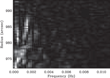
Figure 2. Power spectrum of the relative density fluctuations as a function of height. Here the power spectrum is normalized by the total power at each height. The color scale is linear with a maximum value of 0.15 shown in white and zero in black.
Download figure:
Standard image High-resolution imageThe magnitude of each peak has, in principle, an uncertainty of 100% (Press et al. 1992). This is because for a time series with N data points, the Fourier analysis determines the amplitude and phase at N/2 frequencies. In order to reduce the uncertainty it is necessary to average the power spectra. For example, a common choice is to bin the power spectrum in frequency. In order to preserve frequency resolution, we chose instead to average the power spectrum over the observed height range. This relies on the assumption that the power spectrum does not vary systematically with height. This appears to be the case based on Figure 2, where although there is some structure in the power spectrum versus height there is no clear trend. As our analysis was performed over 64 vertical spatial pixels, there are 64 measurements of the power spectrum, so the uncertainty in the average power spectrum is reduced to about 13%.
3.1.2. Velocity Fluctuations
Velocity fluctuations δv are observed as Doppler shifts of wavelength, δλ. We obtained a stationary time series by fitting λ(t) at each height, y, with a linear trend and determined the fluctuation relative to that trend. For the power-spectrum analysis of velocity fluctuations, we work directly with the wavelength data, δ λ(t, y), as the absolute magnitude of the power spectral peaks is not important. The typical rms amplitude of the wavelength fluctuations was about 0.012 Å. As δ v = c δ λ/λ0, where c is the speed of light and λ0 = 1394 Å; this corresponds to an rms velocity amplitude of about 2.6 km s−1. However, previous studies have shown that Doppler shift measurements of velocities underestimate the actual wave amplitudes due to the line-of-sight integration (McIntosh & De Pontieu 2012) and so are considered to provide a lower limit for the wave amplitudes. The Doppler shift measurements reveal the relative power spectrum, but absolute wave amplitudes are better estimated using line widths (see Section 3.3).
We obtained the Fourier power spectrum for δ λ(y, t) at each height using the same methods as for the intensity fluctuations (Figure 3). Again, there did not appear to be a trend in the power spectrum with height. So, the average velocity fluctuation power spectrum was found by normalizing the power spectrum at each height by the total power at that height and then averaging the normalized spectra over the studied height range.
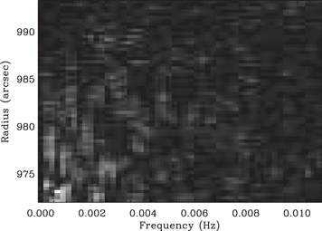
Figure 3. Same as Figure 2, but for the relative velocity fluctuations. The color scale is linear with a maximum value of 0.12.
Download figure:
Standard image High-resolution image3.2. Frequency Relation
The power spectrum for the density fluctuations, Pδ n (f), resembles the power spectrum for the velocity fluctuations, Pδ v (f), and they appear to differ only by a scaling of the frequency axis (Figure 4). Note that, as these power spectra were derived from the same number of underlying data points and were analyzed in the same way, the frequency axes are identical. In order to quantify the frequency scaling, we calculated a correlation coefficient between the two power spectra as a function of a scaling factor applied to the Pδ n (f) frequency axis. To calculate this correlation, we multiply the frequency axis for Pδ n (f) by a scaling factor α to obtain Pδ n (α f), which expands or contracts the power spectrum. As the frequency scale f is discrete, we would like the α f frequency values to match up with f frequency values, so it is necessary to interpolate Pδ n (α f) back to the original f axis. Once that is done, we compute the correlation coefficient, c, between the scaled Pδ n and original Pδ v spectra using the standard formula (e.g., Jenkins & Watts 1968)
where x and y represent the two quantities being compared,  and
and  are their average values, and N is the total number of data points. This correlation coefficient was repeated for a range of α values.

Figure 4. Average power spectrum for the density fluctuations (labeled δn; dotted curve), velocity fluctuations (labeled δv; dashed curve), and line width fluctuations (labeled δw; dashed–dotted curve), normalized to their respective maximum values. The solid curve shows the average power spectrum for the density fluctuations when its frequency axis is multiplied by a factor of 2. In that case, the peaks δn power spectrum align better with peaks in the δv and δw power spectra. The relative uncertainties in the normalized power are estimated to be about 13%.
Download figure:
Standard image High-resolution imageThe solid curve in Figure 5 shows the correlation coefficient between the power spectra for the δn and δv fluctuations as a function of the density power spectrum frequency scaling factor. Figure 5 shows the results for the Si iv 1394 Å line, but we also performed the same analysis for the 1403 Å line. In order to check the sensitivity to our averaging procedure, we also performed the same analysis on power spectra where we weighted the spatial averaging by the statistical significance of the peaks. In all cases, we found similar results. Based on the average peak location in all of the c(α) plots, we found α = 2.01 ± 0.12.
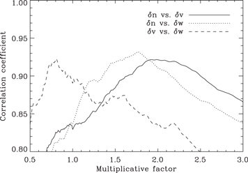
Figure 5. Correlation coefficient vs. scaling factor for the frequency axis for the power spectra of δn vs. δv (solid curve), δn vs. δw (dotted curve), and δv vs. δw (dashed curve). In each case, it is the first variable listed whose frequency axis is to be multiplied.
Download figure:
Standard image High-resolution image3.3. Line Widths and Line Width Fluctuations
The width, w, of a spectral line is set by instrumental broadening, thermal broadening, and nonthermal broadening  . Throughout, all widths refer to the 1σ Gaussian width. The median Si iv line width measured by IRIS in the off-limb region studied here was w = 0.12 Å. IRIS has winst = 0.011 Å (De Pontieu et al. 2014). The peak formation electron temperature for Si iv is Te = 8 × 10⁴ K (Dere et al. 2019). Assuming that the ion temperature is equal to the electron temperature, the corresponding estimated Si iv thermal width is wth = 0.023 Å. Thus, the IRIS line width is dominated by wnt. This nonthermal broadening is caused by unresolved fluid motions along the line of sight, such as due to waves. After subtracting the estimated instrumental and thermal width and converting to velocity units, we find that the median wnt = 24.2 km s−1. This can be interpreted as an estimate of the Alfvénic wave amplitude. Using a line width to estimate the wave amplitude is a more reliable estimate than using the Doppler shift, which only provides a lower limit for the wave amplitudes, as the broadening is not washed out by the line-of-sight integration (McIntosh & De Pontieu 2012; Pant et al. 2019). On the other hand, other flows can also contribute to wnt, so one can conservatively consider wnt to be an upper bound for the wave amplitudes.
We also observed fluctuations in the line width around the average value discussed above. The power spectrum of these δw fluctuations was analyzed using the same methods as for the intensity and wavelength. Figure 6 shows the δw power spectrum as a function of height, which has a frequency distribution that resembles that of the δλ fluctuations shown in Figure 3. Figure 5 illustrates the correlation analysis for the frequency scaling, which shows that the frequency scaling between the δv and δw fluctuations is 0.81, while the frequency scaling for δw versus δn fluctuations is 1.8. So, the δv and δw fluctuations have a similar power spectra, while the power spectra for the δn and δw fluctuations appear to have the same nearly factor of 2 frequency scaling that we previously found for the δn versus δv fluctuations. The rms amplitude of the δw fluctuations was about 0.01 Å, which corresponds to a velocity of 2.2 km s−1. This is very similar to the 0.012 Å amplitude of the Doppler shift fluctuations.

Figure 6. Same as Figure 2, but for the line width fluctuations. The color scale is linear with a maximum value of 0.13.
Download figure:
Standard image High-resolution imageAll of these results suggest that δw and δλ measure the same underlying fluctuations. One possible explanation is that they are both independently showing properties of the Alfvénic waves in the transition region. The δλ Doppler shift fluctuations might show oscillations back and forth along the line of sight, while the δw fluctuations may show broadening from structures where the back and forth motions are not resolved within a single pixel, for example due to unresolved small rotating structures. Another possibility is that the relation between δw and δλ is due to multiple flow components along the line of sight that are not resolved in our single-Gaussian fits. For example, if much of the plasma is stationary, but a fraction is Doppler shifted, the actual line would be a large Gaussian peak blended with a smaller slightly shifted Gaussian. When a single-Gaussian model is fit to such a line profile, the result will be an apparent Doppler shift in the line centroid and a slightly broader line width. Inspection of the fits did not reveal any clear evidence for two-Gaussian functions, but as the Doppler shifts are small compared to the line widths any secondary components may be difficult to resolve. From a pragmatic perspective, the δw fluctuations do not provide any information that is not already less ambiguously provided by the δλ analysis. So, it is not necessary to resolve the issue here.
3.4. Fluctuation Speeds
3.4.1. Density Fluctuations
We measured the propagation speed of the density fluctuations using both time-domain cross-correlation and frequency-domain cross-spectrum techniques. For the cross-correlation approach, we computed the cross-correlation function for δ I(t, yi ) at each height yi , with all larger heights δ I(t, yj ). The lag time τij at which the cross correlation peaks represents the travel time of the wave to go from yi to yj . We quantify τij as the first moment of the peak in the cross correlation and take the uncertainty to be the second moment of the peak. This gives us the lag time as a function of the height difference, τij (Δyij ). For each initial position i, we perform a linear least squares fit to τij versus Δyij , whose slope represents the propagation speed. We found that the cross correlation loses coherence after about 5 Mm, so we performed the fit over a height range of 4.5 Mm. From this method we found the density fluctuation velocity was vδ n = 75 ± 10 km s−1.
We also used the cross-spectrum method to estimate the velocity (i.e., phase speed) of the density fluctuations (Athay & White 1979). The cross spectrum gives the phase difference Δϕij (f) of the fluctuations between two heights yi and yj as a function of the frequency f. The time delay is then Δϕij (f)/(2π f). By computing the cross spectrum between each pair of heights, we inferred the delay time between those heights and then perform a linear fit to find the velocity (Figure 7), just as we did for the cross correlation. The advantage of the cross-spectrum method is that it can, in principle, measure dispersion in the fluctuations, i.e., identify whether the phase speed depends on the frequency. A disadvantage is that resolving the data along the frequency dimension increases the statistical uncertainty. For these data, the uncertainties were large enough that we cannot conclude anything about dispersion. Instead, we focus on a couple of peaks in the power spectrum (Figure 2) to find the velocity. We found that for the peak at f = 5.9 mHz vδ n = 75.4 ± 6.3 km s−1 and for f = 1.08 mHz vδ n = 97 ± 43 km s−1.

Figure 7. Wave travel time Δt versus height difference Δy derived from the cross-phase analysis for the intensity fluctuations at 5.9 mHz. The circles show the data derived from following the eight lowest pixels in the data set over a distance of 20 pixels. The solid line illustrates the average inferred wave speed of 75.4 km s−1.
Download figure:
Standard image High-resolution imageBased on these two methods, the phase speed for the density fluctuations was found to be about 75 km s−1. This can be compared to the theoretically expected sound speed,  , where γ = 5/3 is the adiabatic index, kB is the Boltzmann constant, and mi is the average ion mass. We take mi = 1.15 mp, with mp the proton mass, in order to account for a 5% helium concentration. This expression for cs also assumes that the ion temperature is equal to the electron temperature, which we estimate as the Si iv formation temperature of 8 × 10⁴ K; the expected sound speed is cs = 44 km s−1. So our measured vδn is similar too, though larger than, the expected sound speed. One possible explanation for the discrepancy is that the transition region may be multithermal or not in ionization equilibrium, so that the actual temperature could be larger than our rough estimate based on the Si iv formation temperature.
3.4.2. Velocity Fluctuations
The velocity fluctuations propagate much faster than the density fluctuations, so that they appear as nearly vertical lines in a height—time diagram. The very small travel times or phase delays between two heights and the uncertainties in the data, precluded a cross-correlation or cross-spectrum analysis. Instead, we quantified the phase speed by tracking the motion of features in the height—time plot (Figure 8). Moving features were initially identified by eye. Then, the time at which the feature was present at each height was determined by finding the centroid position (first moment) of the feature along the time axis. We performed a linear fit to the centroid time versus height in order to find the velocity of each identified feature. Based on eight identified features, we found a weighted mean speed of the velocity fluctuations of vδ v = 250 ± 20 km s−1. One should be cautious about taking this number to be too precise, due to the potential for systematic bias in the feature identification step.
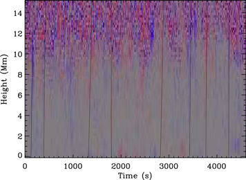
Figure 8. Time–distance plot of δλ fluctuations, which are proportional to δv fluctuations. The color scale is linear from ±0.34 Å, with red negative, blue positive, and gray zero. Black lines show the fit to tracked moving structures in the time–distance plot. The slopes of these lines indicate the speed.
Download figure:
Standard image High-resolution imageThis estimated speed is similar in magnitude to what is expected for Alfvén waves. The Alfvén speed is  , where B is the magnetic field strength, and ρ is the mass density. We take the mean particle mass (including electrons and ions) to be 0.6mp in the corona. Then for B ≈ 4 G and ne = 2.6 × 109 cm−3 (as described in the next section), we estimate VA ∼ 220 km s−1 s−1.
This estimate also confirms the suspected problem with the short travel times through the limited observed height range. As the vertical pixels span a height of 0.24 Mm per pixel and the cadence is Δt = 9.33 s, the theoretical Alfvén speed implies that the Alfvén waves move at a speed of about 7.3 vertical pixels per frame. The measured height range spans 64 vertical pixels, but the useful height range is more strongly limited by noise level. As a result, Alfvén waves are nearly vertical lines in the height—time plot, as we observe. We can say with confidence that the velocity fluctuations are significantly faster than the density fluctuations.
The empirical value for the Alfvén speed allows us to estimate the amplitude of the Alfvén wave relative to the average magnetic field, δ B/B0. For an Alfvén wave δ v/VA = δ B/B0. Thus, the estimated range for δB/B = 0.01–0.1, where the minimum value is based on the Doppler shift fluctuations, and the maximum value is based on the average line width.
3.5. Plasma Properties
We measured the density using the ratio of two O iv lines (Polito et al. 2016). In particular, we used the ratio of the 2s2 2p2 P1/2 − 2s 2p2 4 P1/2 transition at 1399.78 Å to 2s2 2p2 P3/2 − 2s 2p2 4 P5/2 transition at 1401.16 Å. There is a weak photospheric line in the wing of the 1401.16 Å line, but in the off-limb data both lines are unblended.
In order to use the O iv line intensity ratio as a diagnostic we first performed an absolute calibration of the IRIS data to convert from DN to intensity units (Tian et al. 2014a; Wülser et al. 2018). The intensities were then extracted from the spectrum in two ways. In one method, we fit Gaussian line profiles to the O iv lines in order to extract the amplitude, line width, and centroid. However, for low intensities the data are noisy, and the fits may be less reliable. To address that problem, we also integrated the spectrum directly to obtain the total intensity. Both methods resulted in similar intensity ratios and densities. To interpret the intensity ratio as a density, we used the CHIANTI atomic database (Dere et al. 1997, 2019).
Density measurements were most consistent in the height range between 970'' and 980''. Presumably because the lines were brightest at those lowest heights and the density there lies within the range at which the diagnostic is most sensitive. We found that the weighted mean density was  based on the Gaussian fit method and
  , based on the direct integration method. That is, ne = 2.6 ± 0.3 × 109 cm−3.
A potential systematic uncertainty is that the O iv formation temperature of 1.4 × 10⁵ K is somewhat higher than that of Si iv at 8 × 10⁴ K. There is not a sufficient range of ion species to perform a detailed temperature analysis, and the transition region is probably multithermal. Our results do not depend sensitively on the temperature, so wherever an estimate is needed we take Te ≈ 8 × 10⁴ K.
For comparing to theory, it is useful to estimate the plasma β, which is given by β = 8π ne kB Te/B2. Using our inferred density and estimated temperature, we find β = 0.73/B2, where B is the magnetic field strength in Gauss. We do not have a direct measurement of the polar magnetic fields. However, published estimates suggest that the magnetic field strength is in the range of 2–6 G (Tian et al. 2008; Wang et al. 2009; Janardhan et al. 2018). The corresponding range is β ≈ 0.02–0.18.
4. Comparison of Observations with PDI Theory
The apparent frequency-scaling relationship between the density and velocity fluctuations suggests that these oscillations are coupled to one another. One possibility is that this interaction occurs via PDI. Here, we discuss the observations in this context and show that they are consistent with theoretical predictions for PDI.
In PDI, a forward propagating pump Alfvén wave decays into a forward sound wave and a backward Alfvén wave. Our observations are consistent with seeing the pump wave and the secondary sound wave. Based on their speeds, the observed fluctuations are consistent with the density fluctuations representing sound waves and the velocity fluctuations being Alfvén waves. We found that the density fluctuations propagated at about 75 km s−1, which is similar to the expected sound speed. The velocity fluctuations propagated at about 250 km s−1, which is about the expected Alfvén speed. The expected backward propagating secondary Alfvén wave is not clearly seen, but it may be obscured because of its smaller amplitude and because the direction of propagation is difficult to resolve given the fast phase speed and limited height range.
In order to make a more detailed comparison with the predictions of the theory of PDI, we have numerically solved the dispersion relation for PDI from the theory of Derby (1978). This theory is based on magnetohydrodynamics (MHD) with a uniform background magnetic field, B0, and β not necessarily small. The equilibrium state of the plasma also includes a circularly polarized pump Alfvén wave of finite amplitude δ B, frequency ω0, and wavenumber k0, related by VA = ω0/k0. The dispersion relation for PDI is found by linearizing the MHD equations for parallel propagating fluctuations from this equilibrium state. This dispersion relation is given in Equation (17) of Derby (1978), which is a nonlinear algebraic equation involving a fifth-order polynomial of ω and k, which are the frequency and wavenumber of the daughter mode, respectively. There are two parameters, β and δ B/B0, in the dispersion relation.
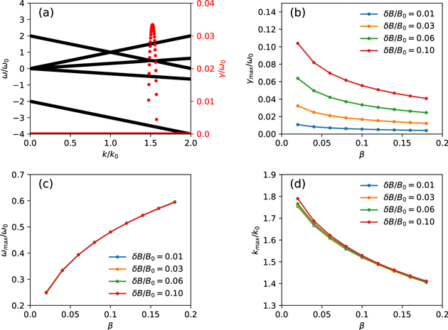
For discrete values of real k, we solve the dispersion relation numerically to obtain solutions for complex ω. The real part of ω is the real frequency of the daughter mode, while the imaginary part γ is the exponential growth rate for the amplitude of the mode. The growth rate for PDI depends on the two parameters, δ B/B0 and β (Derby 1978; Goldstein 1978). Figure 9(a) shows one example of this solution for δ B/B0 = 0.06 and β = 0.1, which are plausible parameters based on the observations. Figures 9(b)–(c) are plotted by solving the dispersion relation for a range of other values of δ B/B0 and β.
Figure 9. (a) Numerical solutions to the nonlinear dispersion relation for parametric decay instabilities of an Alfvén wave (Derby 1978) with δ
B/B0 = 0.06 and β = 0.1. The black dots, which blend together to appear as black lines, show real frequencies ω, and the red dots show growth rates γ, both of which are normalized to the frequency of the pump Alfvén wave ω0. The wavenumbers are normalized to the wavenumber of the pump wave k0 (note that ω0 = k0
VA
). At any given k there are five solutions, most of which are stable (i.e., γ = 0). The unstable solution near k/k0 = 1.53 corresponds to PDI, with a maximum growth rate ∼0.032, and frequency ∼0.48. (b) Growth rate, (c) frequency, and (d) wavenumber of the most unstable (largest γ) PDI mode for various combinations of δ
B/B0 and β. All three quantities depend on β, but  and kmax have little dependence on δ
B/B0. (In (c) four curves lie on top of one another.)
and kmax have little dependence on δ
B/B0. (In (c) four curves lie on top of one another.)
Download figure:
Standard image High-resolution image
Figure 9(b) shows the maximum growth rate for PDI for various combinations of δ B/B and β and demonstrates that the growth rate is largest for large pump wave amplitudes δ B/B0 and low β. This is also consistent with the theory of Sagdeev & Galeev (1969), which for the limit of small amplitudes and small β predicts γ/ω0 ≈ (1/2)(δ B/B0)β−1/4.
Figures 9(c) and (d) plot the frequency  and wavenumber
  , for which the maximum instability growth rate occurs. In both cases, these quantities are normalized by the frequency and wavenumber for the pump wave. Panels (c) and (d) show that
  and
and  depend almost entirely on β and not on the wave amplitude. For low β,
  (Sagdeev & Galeev 1969).
As the sound wave is produced by PDI, it is expected that the sound waves will be excited most strongly at the frequency  . Observationally, we found that the ratio
  . Figure 9(c) indicates that this corresponds to β ≈ 0.1. Our measured and estimated values for density, temperature, and magnetic field imply a range for β = 0.02–0.18. So, the β implied by the theory of the PDI based on the ratios of the observed fluctuation frequencies is in the middle of the estimated range based on our independent estimates of plasma properties.
Assuming the fluctuations are driven by PDI, we can estimate the growth rate from the measured wave amplitudes. The Alfvén wave amplitude can be expressed in terms of the velocity as δ B/B0 = δ v/VA. The rms amplitude of the velocity fluctuations from Doppler shift was 2.6 km s−1, which combined with VA ≈ 250 km s−1 gives an Alfvén wave amplitude of δ B/B0 ≈ 0.01. This is a lower bound as the line-of-sight integration tends to wash out the Doppler shifts. Using the average line width instead, we inferred a nonthermal velocity of vnt = 24.2 km s−1, corresponding to δ B/B0 ≈ 0.1. This is an upper bound, because the nonthermal velocity can be influenced by flows other than waves. As shown in Figure 9(b), the maximum growth rate of PDI is in the range from 0.005ω0 to 0.10ω0, depending on the wave amplitude and plasma beta. Taking observationally plausible values of β = 0.1 and δ B/B0 = 0.06, the growth rate of the PDI is about 0.035ω0. In absolute units, this is 2 × 10⁻⁴ s−1 for a pump Alfvén wave with a frequency of 10−3 s−1.
Although the observational evidence is consistent with PDI, the slow growth rate of the instability and the possible presence of large gradients in this region raise a challenge for this interpretation. For an VA = 250 km s−1 and growth rate γ = 2 × 10⁻⁴ s−1, the wave propagation length during a growth time is about 103 Mm, of order ∼ R⊙. The temperature, density, and magnetic field gradients in the corona are expected to have length scales shorter than this. Under these conditions, we expect the properties of PDI to be modified from the linear theory used above.
There are few theoretical studies of PDI in inhomogeneous plasmas (Tenerani & Velli 2013; Shoda et al. 2018). Tenerani & Velli (2013) have studied PDI numerically, using an expanding box model to discern the effects of solar wind expansion on the PDI. They found that expansion tends to reduce the growth rate, because the resonance condition changes as the solar wind flows outward. Numerical studies under conditions relevant to the lower solar atmosphere are needed in order to understand the effects of inhomogeneity in the observed region.
We should consider whether there are alternative interpretations of the observations other than PDI. One possibility is that the relation between the density and velocity fluctuations is the manifestation of some underlying wave mode having a velocity fluctuation at a harmonic of the compressional oscillation. There is strong evidence against this possibility as such a mode should have a single phase speed so that both the velocity and density fluctuations should move at the same speed, whereas here we find that the velocity fluctuation is significantly faster than the density fluctuation. Still, the velocity fluctuation speed is not measured as precisely or systematically as the other quantities discussed here, which is a systematic uncertainty that future measurements should aim to resolve.
It is also possible that the Alfvénic waves and density fluctuations are not directly coupled, but that the frequency relation arises as part of an unknown process that would excite both types of waves at lower heights. This possibility could potentially be distinguished from PDI by observing the direction of propagation of the Alfvén waves. PDI predicts both upward and downward propagating Alfvén waves, but in the absence of PDI we expect the waves to be propagating upward only. This assumes that there are no other sources of reflection and downward propagating waves besides PDI. Our analysis was not able to resolve this issue. The structures identified for the velocity fluctuation speed analysis were predominantly upward, presumably representing the pump Alfvén waves, although the height—time diagram also appears to show some downward moving fluctuations. In fact, the dominance of upward Alfvén waves in the process of PDI was also observed in numerical simulations (Li et al. 2022). To measure the power in both upward and downward propagating waves systematically, one could apply a two-dimensional Fourier analysis to the height—time diagram to generate a wavenumber–frequency (k − ω) diagram (see, e.g., Tomczyk & McIntosh 2009). Such an analysis was not possible for this data set due to the noise level and the limited height range, which limits the minimum resolvable wavenumber.
5. Conclusions
We find evidence for the first observation of PDI in the lower solar atmosphere near the transition region. Our analysis shows that the power spectrum of density fluctuations matches the power spectrum of the velocity fluctuations except for a scaling of the frequency axis. This scaling factor matches the frequency relationship between a pump Alfvén wave and the secondary sound wave it is theoretically expected to drive via PDI given the estimated plasma β estimated for the observed region.
Other possible processes that could explain the observed relation between the density and velocity fluctuations are that they are due to the same underlying wave mode or that the relation arises due to nature of the wave excitation process at lower heights. The wave mode hypothesis is unlikely, as the density and velocity fluctuations appear to be propagating at very different speeds. An explanation in terms of some unknown wave excitation process cannot be ruled out based on these observations. That possibility could be resolved by better quantifying the power in upward versus downward waves in future work. Developments in theory are also needed to understand how the inhomogeneity of the plasma properties in this region affect the properties of the PDI.
The observation of PDI in the transition region of the Sun has implications for broader models of turbulence and coronal heating. The observed region studied here is a fairly generic observation of the transition region at the base of a coronal hole, so it is likely that PDI is ubiquitous in such regions. This would support numerical models for coronal heating and solar wind acceleration (e.g., Shoda & Yokoyama 2016) that suggest PDI as a mechanism for promoting turbulence and heating. Future work should look for PDI in other structures. If PDI is indeed common, then PDI may be a fundamental process in the Sun that mediates the transfer of energy into the corona.
M.H. and D.W.S. acknowledge support from NSF STR grant 1384822 and NASA LWS grant 80NSSC20K0183. X.F. is supported by NASA LWS grant 80NSSC20K0377.