


Abstract
Rossby waves are found at several levels in the Sun, most recently in its supergranule layer. We show that Rossby waves in the supergranule layer can be excited by an inverse cascade of kinetic energy from the nearly horizontal motions in supergranules. We illustrate how this excitation occurs using a hydrodynamic shallow-water model for a 3D thin rotating spherical shell. We find that initial kinetic energy at small spatial scales inverse cascades quickly to global scales, exciting Rossby waves whose phase velocities are similar to linear Rossby waves on the sphere originally derived by Haurwitz. Modest departures from the Haurwitz formula originate from nonlinear finite amplitude effects and/or the presence of differential rotation. Like supergranules, the initial small-scale motions in our model contain very little vorticity compared to their horizontal divergence, but the resulting Rossby waves are almost all vortical motions. Supergranule kinetic energy could have mainly gone into gravity waves, but we find that most energy inverse cascades to global Rossby waves. Since kinetic energy in supergranules is three or four orders of magnitude larger than that of the observed Rossby waves in the supergranule layer, there is plenty of energy available to drive the inverse-cascade mechanism. Tachocline Rossby waves have previously been shown to play crucial roles in causing seasons of space weather through their nonlinear interactions with global flows and magnetic fields. We briefly discuss how various Rossby waves in the tachocline, convection zone, supergranule layer, and corona can be reconciled in a unified framework.
Export citation and abstract BibTeX RIS

Original content from this work may be used under the terms of the Creative Commons Attribution 4.0 licence. Any further distribution of this work must maintain attribution to the author(s) and the title of the work, journal citation and DOI.
1. Introduction
Rossby waves are a form of inertial wave, found somewhere in all rotating spherical bodies containing fluid, particularly on or in rotating planets and stars. The restoring forces in all inertial oscillations are the combination of Coriolis force and pressure gradient forces. Rossby waves generally propagate in longitude, with the direction of propagation determined by other properties, such as the thickness of the spherical shell as a fraction of the radius of the body. Rossby waves were first recognized for the Earth's atmosphere (Rossby 1939), and are well known to occur in oceans, probably also in the Earth's liquid core (Hide 1966; Raphaldini & Raupp 2020), and in other planetary atmospheres. Light curves of Kepler space mission recently showed the indication of Rossby waves near the surfaces of many stars with different spectral types (Van Reeth et al. 2016; Saio et al. 2018). The waves could also be important in the dynamics of many different astrophysical objects (Zaqarashvili et al. 2021). Rossby waves are central to modern numerical weather prediction models, and are critical for understanding and predicting evolving patterns of solar magnetic activity.
Since the first discovery of solar Rossby waves (McIntosh et al. 2017; Loptien et al. 2018) a rapidly growing amount of evidence has shown that the Sun also contains Rossby waves (Hanasoge & Mandal 2019; Liang et al. 2019; Mandal & Hanasoge 2020; Hathaway & Upton 2021); it is then very likely that other stars with convection zones also contain them. An earlier report of evidence of solar Rossby waves by Kuhn et al. (2000) has been shown by Williams et al. (2007) to instead be evidence of corrugations in the lower solar atmosphere from supergranules below. Evidence of Rossby waves has now been seen in both solar velocities and magnetic structures in the solar atmosphere. Near-surface helioseismic measurements have revealed them, as have surface flow fields and patterns. Global coronal brightness patterns and coronal bright points show evidence of Rossby waves. There are differences between the velocity and magnetic feature measures of Rossby waves, but such differences could in part be evidence of Rossby waves originating in different depths in the Sun's photosphere, and below and above as well. There is also theoretical and modeling evidence of Rossby waves in the solar tachocline, which plausibly are generated due to global magnetohydrodynamics there (Dziembowski & Kosovichev 1987; Gilman & Fox 1997; Dikpati & Gilman 2001; Zaqarashvili et al. 2010; Balk 2014; Raphaldini & Raupp 2015; Dikpati et al. 2018a), and nonlinearly interact with the spot-producing toroidal magnetic fields and differential rotation to cause the short-term seasonal or quasi-annual/quasi-biennial variability observed in the surface solar activity and space weather (Dikpati et al. 2017, 2018b).
It is well known from theory and models that Rossby waves have different properties, particularly their longitudinal direction of propagation and their frequency, as functions of longitudinal wavenumber, depending on the thickness of the layer they reside in compared to the radius of the rotating body. All Rossby waves arise from the conservation of potential vorticity as fluid particles move in a rotating fluid. Potential vorticity is defined as the fluid vorticity measured in an absolute frame of reference, divided by the product of the fluid shell thickness and the fluid density. In a thin 2D fluid shell such as the Earth's lower atmosphere neither thickness nor density variations are important, so potential vorticity varies in the same way as absolute vorticity, and all models show that Rossby waves propagate retrograde relative to the rotating frame because fluid particles displaced toward the equator spiral to the west against the rotation direction. By contrast, fluid columns aligned with the axis of rotation in a thick fluid shell outside the tangent cylinder to its inner boundary, whose fluid density, and thickness parallel to the rotation axis, decline in the outward direction, as in a rotating star, lead to prograde propagating Rossby waves (see, e.g., Glatzmaier & Gilman 1981). From both the thickness and density gradients, outward moving fluid columns spiral in the direction of rotation, leading to the prograde propagation. To achieve these prograde Rossby waves requires that the Sun be rotating fast enough so that the flows outside the equatorial tangent cylinder tend to align with the rotation axis. This property has not yet been established in the Sun; it could be that the Sun is simply not rotating fast enough for these particular Rossby waves to be present.
The primary property of Rossby waves that has been detected in the various solar measurements described in the references cited above is their frequency as a function of longitudinal wavenumber. In particular, both helioseismic and surface correlation tracking measurements find the retrograde phase speed, of an amount consistent with the fluid shell in which the waves reside being thin. This means they are like Rossby waves in a thin planetary atmosphere such as the Earth, despite the fact that while the Earth's troposphere is no more than one pressure scale height thick, the outermost layer of the Sun's convection zone is many scale heights deep. In addition, the Earth's troposphere average vertical stratification is subadiabatic, conducive to nearly horizontal flow with nearly hydrostatic balance in the local vertical direction, which leads to flows that are extremely large in horizontal scale compared to the thickness of the layer. By contrast, the outer layers of the solar convection zone have superadiabatic stratification and contain vigorous convection everywhere (granulation), whose flow is certainly neither hydrostatic nor primarily horizontal. Yet Rossby waves characteristic of a thin stably stratified atmosphere are seen. This reveals a form of paradox for the Sun, which we will discuss.
Henceforth in this paper our aim is to explore theoretically the generation of Rossby waves observed in velocities near the top of the convection zone. In our judgment there are only two possible ways such waves can be excited and maintained. One is that they are generated in situ; the other is that they propagate up to the top from wherever they are generated below. Here we focus on in situ generation. Separately, upward propagation of Rossby waves generated below is under study. In situ generation of Rossby waves requires an in situ energy source. One possibility is the Sun's latitudinal differential rotation, which could be unstable to Rossby waves. In that case, the Rossby waves would be energetically active, taking kinetic energy from the differential rotation, which itself would have to be maintained by some other mechanism. This would require Reynolds stresses (correlations between longitude and latitude motions) that transport angular momentum from low latitudes to high, down the gradient of angular velocity. But all theoretical models for the differential rotation do exactly the opposite, transporting angular momentum toward the equator to maintain it against turbulent diffusion by smaller scales. And measures of angular momentum transport by flows, such as correlations of longitude and latitude motions of sunspots (Gilman & Howard 1984), also show angular momentum transport toward the equator, but being a magnetic measure, these data may be reflecting flow correlations coming from much deeper levels of the convection one. Furthermore, the Rossby waves observed through their associated fluid velocities appear to be energetically neutral; that is, they have no Reynolds stress associated with them. So there must be some other energy source to excite and maintain Rossby waves. Here we explore whether the horizontal motions in supergranulation can provide this energy source.
2. Rationale for Supergranulation as the Excitation Source of Rossby Waves
So how can the apparent paradox of finding Rossby waves with virtually horizontal motion in a fully convective medium be resolved? Stated another way, while stable stratification of a thin rotating spherical shell is sufficient to result in Rossby waves, given an excitation mechanism, it may not be necessary. It is well known that Rossby wave modes with no vertical motion can, at least in theory, even exist in atmospheres of arbitrary vertical density profile (see, e.g., p. 379 of Pedlosky (1987). They are called barotropic modes, and can exist even without requiring hydrostatic equilibrium. Historically in meteorology it has generally been assumed that if unstable stratification is present and the system is experiencing convection (or possibly other small-scale motions), Rossby waves will not be favored. But that does not rule out them being present. Convectively driven Rossby waves have been invoked for deep atmospheres of giant planets (Liu & Schneider 2011) and in more general theory (Tikhomolov 1996). Apparently this is what is happening in the supergranule layer of the Sun. By any measure the kinetic energy of both supergranulation and granulation is orders of magnitude higher than that of the observed Rossby waves. One implication of this fact is that while Rossby waves in the supergranule layer may be useful as diagnostic tools, they are very unlikely to be dynamically significant in the supergranule layer, since there is so much more energy in the much smaller scales of motion.
Given how large the kinetic energy of granulation and supergranulation is compared to the observed Rossby waves, if even a small amount of this energy could leak into global scales of flow, it would be enough to maintain the observed kinetic energy of the Rossby waves in the depths where granulation and supergranulation are found. This transfer of energy from small to large scales is well known to turbulence modelers as inverse cascade, and is well known to occur in stably stratified thin rotating spherical shells. But here too it may not be essential that the shell be stably stratified.
Supergranulation is better suited than granulation to be the source of the energy to excite Rossby waves through the possible inverse-cascade mechanism, for multiple reasons. First, from observations, supergranulation flow is predominantly horizontal flow, as are Rossby waves. The predominance of horizontal over vertical motions in supergranules implies they are rather shallow, perhaps no more than 30 Mm, no more than 4% of the solar radius. By contrast, granulation observations show mostly vertical flow. Second, the horizontal scale of supergranulation is only one order of magnitude smaller than that of Rossby waves (Rossby waves are always global in thin layers, but supergranulation by inspection is not), and granulation is between two and three orders of magnitude smaller in scale. Third, supergranules last long enough (∼1 day) to be modestly influenced by Coriolis forces, but granulation lifetimes are much too short (<10 minutes) to feel that influence. Finally, while there is no doubt that granulation is a form of convection, with many numerical models predicting the scale and turnover time, the same is less clear for supergranulation. There is still some debate about whether it is convection at all. In fact, it has been proposed that supergranulation itself is driven by an inverse cascade of kinetic energy from the even more energetic granulation. Thus, the idea of inverse cascades of energy playing important roles in solar fluid dynamics and MHD in convection zones has already been invoked. Rincorn & Rieutord (2018) have given a recent comprehensive review of observations, models, and theory of supergranulation, which includes the points we have discussed above.
3. Model to Link Supergranules with Rossby Waves
Ideally it would be best to explore whether the inverse cascade of energy from small scale can generate near-surface Rossby waves or not is by using a global high resolution thin shell model for convection, one that fully resolves at least supergranulation, and even granulation. But to our knowledge no such model of this resolution has been used, mainly because it would require far too much supercomputer time (due to the high spatial and time resolution needed) to do a meaningful simulation involving inverse cascade of energy from supergranulation and especially granulation. This is particularly a limitation if supergranulation itself is driven by an inverse cascade from granulation. Also, there does not appear to be any generally accepted theory of supergranulation that correctly predicts its horizontal scale and pattern. So we have chosen a different strategy, using a global model that focuses on horizontal motions and has enough horizontal resolution to include scales of motion that are an order of magnitude smaller than Rossby waves, as supergranulation is.
Note that our aim is not to develop a theoretical model for supergranulation, but to initialize our global model with kinetic energy at only the smallest scales, and explore their dynamical interactions with other global-scale motions. Then the simulation experiments will determine whether an inverse energy cascade is possible in reaching global scales; if possible, how efficient is the inverse-cascade process, and what the properties are of the global motions that are excited. Do they have the right properties of Rossby waves to compare with solar observations? The initial kinetic energy at small scales will contain a lot of horizontal divergence as well as some amplitude in the vertical component of vorticity, just as supergranules do. Finally, we acknowledge that the supergranule layer, unlike the tachocline, is not clearly distinct from the rest of the convection zone below (or above, in the case of the tachocline). However, it is the layer where the convection zone changes from larger scale motions substantially influenced by Coriolis forces (Rossby number <1), to motions that are at most only slightly influenced by Coriolis forces (Rossby number >1). This difference, in its own way, does support the idea of treating it as a dynamically distinct layer in models of solar fluid dynamics.
All of the characteristics described above are included in the hydrodynamic version of the global nonlinear shallow water model of Dikpati (2012). The major difference from the Sun is that this model does not include convection explicitly because it is stably stratified, and it is very limited in vertical resolution, so it only focuses on the shallow-water mode, which is essentially a quasi-3D barotropic mode. Also, there is a close correspondence between the shallow water system and a stratified fluid with an equivalent depth (Pedlosky 1987). What this means is that for each propagating Rossby wave in a stratified fluid there is a wave with the same propagation speed in a homogeneous layer of the equivalent depth. This property was originally derived by Taylor (1936) and it is valid for all wave modes in stratified and compressible atmosphere. This shallow-water layer also contains another form of small-scale motion, also driven by buoyancy forces, namely, horizontally propagating gravity waves. This is important because the model is free to determine whether the kinetic energy introduced at the smallest scales goes into driving a wide range of gravity waves, or it in fact does inverse cascade into global scales to excite Rossby waves, or both. We recognize that there are no actual gravity waves generated in the supergranule layer because it is superadiabatically stratified; we are instead representing in the initial conditions the horizontal motions of supergranules. Therefore, the numerical experiments we will perform are analogous to those we would perform with a fully convective thin shell, but more efficient by orders of magnitude. We think of this approach as an analog to the convection cascade problem, rather than as a form of it. We will report on a series of numerical experiments that include cases with no rotation, solid rotation, and differential rotation to determine the role of rotation and differential rotation for transferring energy to the largest spatial scales from supergranule-like scales.
3.1. Equations
Over the last several decades nonlinear hydrodynamic shallow-water models have been applied for studying global oceanic and atmospheric dynamics (see, e.g., p. 387 of Pedlosky 1987). Such models, as well as the generalized versions, including magnetohydrodynamics, have been extensively applied for studying global solar dynamics (Gilman 2000; Zaqarashvili et al. 2010; Klimachkov & Petrosian 2017; Dikpati et al. 2018b). A full set of nonlinear hydrodynamic and magnetohydrodynamic shallow-water equations, applied to study tachocline instabilities, have been presented in an inertial frame of reference in spherical coordinates (see, e.g., Dikpati & Gilman 2001; Gilman & Dikpati 2002). Here we focus primarily on the hydrodynamic shallow-water system, and present the equations in the rotating reference frame, corotating with the core-rotation rate.
Basic formulation of a global nonlinear shallow-water model, including physical assumptions, approximations, and boundary conditions, applied to the Sun have already been presented in various papers (see, e.g., Dikpati et al. 2018b), which also provide detailed formulations of energy integrals in closed form. We do not repeat them here. In brief, shallow-water models are quasi-3D models with a much larger horizontal extent than thickness. The variations in the horizontal direction are much larger than in the vertical direction. Due to the thinness of the fluid layer compared to radius of the astrophysical body divergence of the radii and the density variation are ignored in the momentum and mass continuity equations. Traditionally, shallow-water models are hydrostatic in the vertical because the horizontal spatial scale of the motions is much larger than the thickness, but it has recently been shown (Jalali & Dritschel 2021) that such models can be extended to include nonhydrostatic motions whose horizontal scale is comparable to the thickness of the layer. We have not employed that extension here, but it may be useful in the future.
Before we write the full set of nonlinear hydrodynamic shallow-water equations in the frame rotating with core-rotation rate (ωc ), we discuss the application of the shallow-water model in our case here. The supergranulation layer of the Sun is thin, with thickness no more than a few percent of the solar radius. Therefore, for the simulations that follow, we use a global thin spherical shell. Its undisturbed thickness varies with latitude according to whether the shell is rotating, differentially rotating, or not rotating. In our case, the variations in thickness are all small, but the dynamical perturbations to the thickness are very important because they allow for gravity waves that can absorb energy put in at the smallest scales of the model, without giving rise to energy transfer to excite global-scale Rossby waves. Thus, in this model the nonlinear mode-mode interactions can choose to inverse cascade and/or to get absorbed in gravity waves.
If we denote λ as longitude, ϕ as latitude, t as time, u as the longitudinal velocity in the rotating frame, v the latitudinal velocity, and h the height deformation of the top surface, then the dimensionless governing shallow-water equations are given by
In Equations (1) and (2) above, the parameter G is no longer a measure of the actual effective gravity of the supergranule layer, but rather a parameter to set the characteristic frequencies of gravity waves present in the model. The dimensional parameters within G, such as the radius, layer thickness, and gravity, have somewhat different values than were originally chosen for the application of the model to the tachocline (radius larger, gravity smaller, thickness in the same range), but the appropriate G values to include gravity waves that are relatively high frequency compared to Rossby waves are in the same range as they were for the tachocline case. Gravity waves in this model have frequencies proportional to G1/2, so the smaller G is, the lower the frequency. We take a G value large enough that the model gravity waves propagate much faster than Rossby waves, so they are quite distinct. We take G = 10 for all cases studied. To evaluate G, we use an estimate of the thickness of the supergranule layer. In order to separate the timescales of Rossby and gravity waves, G just has to be large enough. In this study G has been specified to be of value 10. By following the definition of equivalent height as given in Pedlosky (1987), the thickness of the supergranule layer would be somewhat larger than the equivalent height, since the latter is close to ∼1 scale height. So if we consider an equivalent height of that layer, the value of G would be greater than 10, for which the dynamics of the model will be similar because the behavior of modes was found to change the regime from high G to low G below about G = 1 (Dikpati 2012).
3.2. Solution Method
Nonlinear shallow-water equations have been solved by Dikpati and colleagues using pseudo-spectral schemes. Since the details can be found in Dikpati (2012) (see also Dikpati et al. 2018b), here we briefly describe the major steps, and describe certain small differences in the present simulations compared to that of TNOs (tachocline nonlinear oscillations).
To solve Equations (1)–(3) we perform the following steps: (i) compute u, v, and h in a Gaussian grid of ϕ − λ; certain nonlinear terms are computed in real space and then are converted to spectral space; (ii) for time evolution, first kick-start using the fourth-order Runge–Kutta method, then apply the Adams–Bashforth method; (iii) momentum is checked and balanced every few steps; (iv) in order to avoid ringing/Gibb's phenomena, a small spectral viscosity is added; (v) a semi-implicit scheme is used to integrate the effect of very high-frequency gravity waves. For the length of integrations we have done, the small spectral viscosity added makes no measurable difference in the constancy of the total energy of the system with time. Velocities do not decay in total, which we will see later in the results section while discussing our simulation results.
In the TNO study, Dikpati et al. (2018b) focused on low longitudinal wavenumbers m up to m = 10 or so, and the evolution of the model-system containing spot-producing magnetic fields was advanced for several months. However the present study requires all possible l and m in spherical harmonics representations of u, v, and h. With m ≤ l, we consider all possible m for l up to 21 and 42, respectively, in the T21 and T42 models. The computation is done in a 4.5 petaflop supercomputer "Cheyenne" at the NCAR-Wyoming supercomputer center, using OpenMP parallelization.
To perform a simulation run for 1 day, 500 cpu hours are required in a T21 model. But in a T42 model, this time increases by about a factor of 10. Therefore, we demonstrate only one case of our simulations in a T42 model, and the rest we do using a T21 model. Performing simulations of one case in both resolutions also confirms the validity of the numerical scheme. The T42 model truly captures the supergranule scale, but due to being too expensive, we do almost all our simulations in a T21 model. T21 is not fine enough to truly include supergranule scale horizontal motions; however, if similar results are obtained using both the T42 and T21 models, we can safely use the T21 model for exploring various numerical experiments.
3.3. Initial Conditions
For the initial conditions in all cases below we put kinetic energy in almost all l, m modes to ensure nonlinear interaction, but with the spectrum in m heavily weighted toward the highest wavenumbers m allowed in the model; this spectrum peaks at m = 35 for the T42 model and m = 15 for the T21 version, above which it falls off sharply to the highest m allowed, namely, m = 42 and m = 21, respectively. We also include initial potential energy in the form of undulations of the top surface to further enhance the ability of the model to stimulate gravity waves on all spatial scales.
We compute the radial component of vorticity and horizontal divergence present in the initial motions. We know that Rossby wave velocities are almost all vortex motions with very little divergence. By contrast, supergranule horizontal motions are mostly divergent as estimated from results in Langfellner et al. (2015) and Böning et al. (2015). We select the initial velocities in such a way as to reflect these characteristics of supergranulation. The vorticity ζ and horizontal divergence δ in our initialization are given, respectively, by

and

Since energy is a scalar quantity it is straightforward to compute the kinetic energy in the initial state as a function of m. But the vorticity and divergence, being or containing vectors, can be computed at each grid point of the domain. To compute the mean-square vorticity and divergence as function m at t = 0, we integrate the square of these quantities over the entire domain for each m. A similar methodology is used for the calculation of mean-square vorticity, which is often called enstrophy in fluid mechanics (see, e.g., Weiss 1991; Umurhan & Regev 2004).
How the system responds to the initial kinetic energy at small scales critically depends on the magnitude of the energy. Small initial energy means the nonlinear advection terms in Equations (1) and (2) will always be small compared to horizontal pressure gradients and Coriolis forces, and even compared to local accelerations (∂u/∂t, ∂v/∂t). There will be no preference for Rossby waves over gravity waves modestly influenced by rotation. That is clearly not the situation in the Sun's supergranule layer, where the kinetic energy of horizontal supergranulation flow is three or four orders of magnitude larger than the Rossby waves observed. If the initial kinetic energy in the system is large enough to be responsible for producing significant nonlinear advection terms, mode-mode nonlinear interactions in small-scale motions can lead to a different quasi-stable state in the system. While the nonlinear advection terms in the equations of motion couple modes with different l and different m together to excite other modes with other l, m values, in rotating spherical geometry there is a second mechanism for mode coupling, namely, the Coriolis forces, which couple modes of the same m but differing l values. In the general case, both mode coupling mechanisms operate.
4. Results
4.1. T42 Model Simulation with Solid Rotation
As previewed above, we first carry out a simulation with the high resolution T42 model, which truly captures supergranule scale. Figure 1(a) shows the initial kinetic energy spectrum for this simulation, which peaks around m = 35, similar to where supergranulation energy peaks. Initially, there is essentially no energy at low m. Figure 1(b) shows the initial distribution of squared vorticity and horizontal divergence by wavenumber m, which shows that at the highest m, which represent supergranule scale horizontal motions, the motions have little vorticity compared to their divergence, consistent with observations. In fact, all but the very lowest m modes have more initial divergence than vorticity. And both are small for m < 15 or so compared to higher m. This ensures that initial conditions are not favored for producing large vortical motions.

Figure 1. (a) Initial kinetic energy assigned to each longitudinal wavenumber m (summed over all possible l) at the start of the T42 simulation. (b) Mean-square vorticity and horizontal divergence in initial state for each m.
Download figure:
Standard image High-resolution imageCan the Coriolis forces acting on the small-scale divergent motion generate large vortical motions as the dynamics evolve? Can mode-mode nonlinear interactions carry kinetic energy in wavenumber space from large to small m, where Coriolis forces have much greater influence on the flow?
Three snapshots of the evolving kinetic energy spectra in l, m space are shown in Figure 2. The movie shows their continuous evolution (attached in the caption of Figure 2). The total calculation shown is for 1.7 days. We see that the energy very quickly migrates from high m and l to low m, l, to modes of less than 6,6 or so. Each of these modes contains far more kinetic energy than do high individual m's at the start of the simulation. Thus, we see that an inverse cascade of energy via mode-mode interactions can quickly take energy from supergranule scales and deposit it in global low m modes that are likely to be Rossby waves.

Figure 2. Three snapshots during the evolution of kinetic energy spectra in spectral space, for the initial solid rotation, in a T42 model. Continuous evolution can be seen in the animation movie at https://drive.google.com/file/d/1uF-2GUVu5vgd2CnMoCye-H0D9zgunp6n/view?usp=sharing.
Download figure:
Standard image High-resolution imageThese low m modes now contain mostly vorticity, which is characteristic of Rossby waves. Having obtained the basic inverse-cascade phenomena in a T42 model, several numerical experiments as well as analysis need to be performed to understand the features of these low m modes. However, the T42 model is extremely expensive: producing a 1.7 day run uses 36 cores × 12 hr per run × 45 runs, which is approximately 20,000 core hours. Therefore, for the feasibility of completing the necessary simulations, we do all subsequent simulations reported below with the T21 version of the model, which is roughly 10 times faster. The T21 model can retain all the characteristics of the T42 model, just with less scale separation between the smallest resolved scales and global scales.
4.2. T21 Model Simulation with Solid Rotation
Figure 3 shows the initial kinetic energy spectrum for a simulation at T21 summed over l for each m. For this case the spectrum peaks around m = 15, in contrast to the the T42 case shown in Figure 1, where it peaks near m = 35. We also see in Figure 3 that the vorticity and divergence mean-square amplitudes are similar to those for the T42 case, but of course peaking at a lower wavenumber. For the T21 simulations, the horizontal divergence is initially much larger than the vorticity for all longitudinal wavenumbers.

Figure 3. (a) Initial kinetic energy assigned to each longitudinal wavenumber m (summed over all possible l) at the start of the T21 simulation. (b) Mean-square vorticity and horizontal divergence in initial state for each m.
Download figure:
Standard image High-resolution imageFigure 4 shows a sequence of energy spectra during an evolving solution. Panel (a) shows the spectra shortly after the initialization (about 0.18 day). Here kinetic energy is spread over a wide range of wavenumbers, but concentrated at the high wavenumber end. As time progresses (panels (b), (c)) one can clearly see energy migrating to both low l and low m, and by panel (d) the highest energy concentrations are in l, m at 6,6 and below. By about 2.4 days and onward (see the bottom two panels, (e) and (f), the spectrum is stabilizing with dominant energies present in m = 1−4 with corresponding  . These are most likely global-scale Rossby waves. In the accompanying video, it is possible to see waves of kinetic energy migrating from high to low m with time. This appearance is partly due to potential energy at high m in the initial state being converted to kinetic energy of the same m as the calculation proceeds. This initial potential energy is providing a source of energy more extended over time, but it is also limited by the constraint that the total energy, kinetic plus potential, is pretty accurately conserved in these simulations, very much like what we saw in the TNO simulations (see, e.g., Figure 3(a) of Dikpati et al. 2017).

Figure 4. Snapshots of kinetic energy spectra in spectral space, for initial solid rotation, for T21 simulation runs. Six panels capture the characteristic features of this spectra during time evolution. Continuous time evolution can be seen at https://drive.google.com/file/d/13UlysyOnoYbPnifj3yBiYLeTKYbpbRwm/view?usp=sharing.
Download figure:
Standard image High-resolution imageIt is to be noted that the energy spectra cannot reach a fully stable state because of the presence of large nonlinearity. The spectra reach a quasi-stable state, in which the dominant m = 1−4 modes continue nonlinear exchange of energies among themselves in a slow rate (compare panels (e) and (f) of Figure 4), but no evidence of the energy cascading back to higher wavenumbers is seen even in the longest simulation of 25 day duration. A small difference between the solid rotation simulations performed using a T21 model and T42 model is that in the T21 model the Rossby waves are even more concentrated at the lowest m's, but with very similar overall evolution and final spectral profiles.
Figure 5 shows how kinetic (panel (a)) and potential (panel (b)) energies migrate in m-space as a function of time. In Figure 5(a) we present the kinetic energy for each longitudinal wavenumber m for all possible spherical harmonic indices l and display the evolution of the kinetic energy in a contour plot, in which m is the vertical axis and t the horizontal axis. The constant energy contours in panel (a) show how the kinetic energy is being transferred from high m to low m. The peak in kinetic energy, denoted by yellow in this PARULA color map (dark blue–sky blue–green–yellow), migrates smoothly from wavenumber m = 15 down to a band of energy in wavenumbers 1–4, with a peak at m = 2,3. Note also that only a small or negligible amount of kinetic energy ends up in the m = 0 band, which implies latitudinal differential rotation. This result suggests that in the solar supergranule layer, the inverse cascade of energy from supergranule scales to larger scale does not play a significant role in the generation and sustenance of observed latitudinal rotation gradient. But it has been known for many years that vertical momentum transfers by supergranulation may be responsible in significant measure for the near-surface shear layer observed there (Gilman & Foukal 1979; Hotta et al. 2015; Matilsky et al. 2019). Finally, we note that there appear to be weak bands of kinetic energy at higher wavenumbers that show migration toward both lower and higher m with time. These represent some combination of gravity waves and nonlinear mode-mode interactions that at times are reflecting back toward higher m with time.
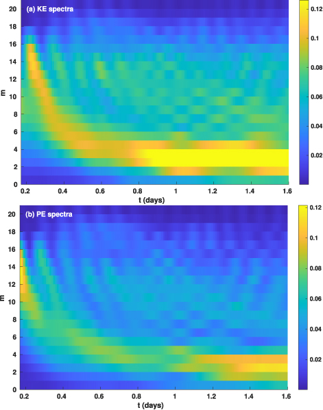
Figure 5. Top and bottom panels respectively display kinetic and potential energies (dimensionless units) in each m (i.e., summed over all possible l's) as function of time, to display inverse cascading with time in T21 simulation runs. In each panel the energy with time in each m is labeled on the left axis at the bottom of that band.
Download figure:
Standard image High-resolution imageWe can see in the bottom panel (b) of Figure 5 that the potential energy also moves from high to low m in spectral space in about the same time interval, but with a small shift in time by about a few to several hours with respect to the movement of the kinetic energy spectra. Note that the shell thickness variations that determine it are closely spatially correlated with the horizontal velocities. This is because Rossby waves are nearly geostrophic, with vortical velocities swirling round high and low pressure centers, consistent with a near balance between horizontal pressure gradient and Coriolis forces.
Figure 6 shows that the total energy, kinetic plus potential, is conserved over the length of the T21 simulation, despite the presence of a small amount of spectral viscosity at the highest wavenumbers. The simulations presented here are essentially for an ideal HD setup. We see several interesting features revealed from Figure 6. First, some out of phase oscillations with time between kinetic and potential energies are evident as the simulation proceeds. This is expected because the kinetic and potential energy reservoirs can nonlinearly exchange energies between them, here in an approximate timescale of gravity waves. We also see that the kinetic energy slowly grows with time at the expense of the potential energy of the system. This is also a clear evidence that the Rossby waves are getting generated in the system. Much longer simulations reported in Dikpati (2012) and Dikpati et al. (2017) show the same precision of total energy conservation of the system.

Figure 6. Evolution of kinetic (red), potential (blue), and total (black) energies (dimensionless units) (summed over all possible l's and m's) as function of time for the T21 simulation runs.
Download figure:
Standard image High-resolution imageWe bring out further properties of the emerging Rossby waves by constructing synoptic maps of the flow and height fields, and by measuring the phase speed of the Rossby wave patterns on these maps. Figure 7 shows a sequence of three synoptic maps of the horizontal flow vectors and the variations in the thickness of the single layer of the shallow-water model. We can see clearly that as time advances, the initial pattern, dominated by small scales, evolves over time to one with global organization of flow and thickness into N-S bands at a much lower wavenumber. These bands are the manifestation of low longitude wavenumber Rossby waves. Over time, there are slow variations in the total pattern, as well as migration of the pattern in the retrograde direction (right to left in Figure 7), which is characteristic of classical Rossby waves. A more detailed analysis reveals that there are nonlinear interactions among these Rossby waves, contributing to time variations in the amplitude of each wave. From such data it may be possible to define lifetimes of individual Rossby waves, in a way analogous to what is done in helioseismological studies of solar acoustic waves.

Figure 7. Three snapshots of synoptic map during evolution of vortical flows (arrow vectors) superimposed on height deformation (color map), for initial solid rotation. Red denotes the height or high pressure relative to equilibrium pressure and blue the depression or low pressure regions. Continuous evolution can be seen in the animation movie available at https://drive.google.com/file/d/1oM-Iq79E8UwfW_--Bc3086APcvvIh41A/view.
Download figure:
Standard image High-resolution imageOur initial flow pattern, concentrated at high m, contained much more horizontal divergence than vertical vorticity. What has changed as a result of the inverse cascade? Figure 8 shows the mean-square vorticity and divergence after about 4 days of simulation. We see that now there is much more vorticity than divergence, especially at low m. This has occurred as a result of Coriolis forces acting on the flow at all m, coupled with the inverse cascade of kinetic energy, which inevitably results in vorticity being concentrated where in m space the velocity amplitudes are the largest. High vorticity compared to divergence is a fundamental characteristic of Rossby waves. Since Figure 8 is a snapshot of vorticity and divergence rather than an average, we should expect the envelope of vorticity amplitudes will not be smooth at any given time. This accounts for the somewhat smaller amplitude in the m = 5 mode compared to its immediate neighbors. At another time, m = 5 might be larger than its neighbors. The nonlinear interactions among Rossby waves with neighboring wavenumbers will continually fluctuate the amplitudes relative to each other.

Figure 8. Evolved mean-square vorticity and horizontal divergence after about 4 days for each m.
Download figure:
Standard image High-resolution imageWe can also see in Figure 8 that there is a small amount of vorticity and divergence in the m = 0 mode. The divergence is associated with the time dependent meridional circulation, obviously much weaker than latitudinal flow for m > 0 modes. Coriolis forces acting on this circulation generates a small amount of vorticity in the small induced differential rotation. This small effect is concentrated in middle and high latitudes where the Coriolis forces are stronger. As can be seen in Figure 8, this feature is quite weak compared to the Rossby waves induced by the inverse cascade.
4.3. T21 Simulation with Differential Rotation
In this section, we simulate the mode-mode interactions when the T21 model is initialized with a differential rotation of the form as derived from helioseismic observations (see, e.g., Charbonneau et al. 1999):

So for these cases we have a prescribed initial differential rotation velocity for the longitudinal motion u for the m = 0 mode, but then we allow the system to evolve as it will according to the nonlinear dynamics, still conserving total energy (kinetic plus potential energies) of the system.
For G = 10, we know that the differential rotation given by Equation (7) is hydrodynamically stable to perturbations unless s4 is large compared to s2. When we simulated the nonlinear interactions among large m modes, including a pole-to-equator differential rotation of 28% equally contributed by s2 and s4 terms, we get very similar results to those with no differential rotation because this differential rotation is stable. A very similar inverse cascade of kinetic energy occurs in this case, but the Rossby wave longitudinal phase speeds are altered somewhat by the presence of the differential rotation.
The case with unstable differential rotation is more interesting. For this case we distributed the same 28% pole-to-equator differential rotation contributed by s2 and s4 terms as s2 = 0.04 and s4 = 0.24. This profile is unstable with perturbation e-folding growth time of about 5 months. Figure 9 shows the kinetic energy spectrum plotted in l, m space, analogous to that shown in Figure 4 for the case of solid rotation. We again see evidence of an inverse energy cascade, but one that appears less vigorous than without differential rotation present, in that kinetic energy is somewhat less concentrated at the very lowest wavenumbers, and with somewhat more energy remaining in the high wavenumbers. What is happening here is that the kinetic energy is coming into low l, m modes both from higher l, m and from the differential rotation itself, resulting in some oppositely directed energy cascades, leading to peak energy for modes l, m of 3 and 4, rather than 1 and 2 as in Figure 4. In some sense, the low m modes 1 and 2, which are unstable, push back against the inverse energy cascade.
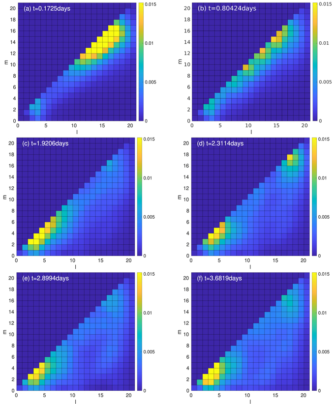
Figure 9. T21 model evolution of kinetic energy spectra in spectral space, for a pole-to-equator differential rotation of 28% that is unstable to hydrodynamic perturbations.
Download figure:
Standard image High-resolution image4.4. Longitudinal Phase Speeds for Rossby Waves with Different Background and/or Initial States
We can estimate the phase speed in longitude for each longitudinal wavenumber m from synoptic maps made at a sequence of times, and tracking the distance each peak in vorticity or thickness moves. We do this by creating images of velocities filtered for each m mode, in which all l's are present. Because the system is nonlinear, the movement is not always at the same speed, and there are amplitude changes as well, arising from various mode-mode interactions due to the nonlinear fluid advection terms in the equations of motion. Gravity waves also cause occasional rapid movements in latitude, during which the tracked vortex pattern may fade out and reappear. Therefore, a phase-speed estimate is a formidably difficult task. However, we manage this by tracking simultaneously a few vortices, so that all do not fade out at the same time. Thus, the estimates are reasonably stable, and consistent with each other. We compare all phase speeds measured in this way with the classical Rossby wave formula for phase speed, originally derived by Haurwitz (1940), given in dimensional form as

in which Ωc is the rotation rate of our coordinate system, and as above, l is the spherical harmonic index.
Figure 10 shows measures of the westward (retrograde) propagation speeds of Rossby waves with longitudinal wavenumbers between 1 and 10, all measured dimensionally in units of degrees of longitude per day, a familiar measure for solar rotation observations. The classical Rossby wave speed is denoted with black filled circles, together with two cases starting from solid rotation, one with large initial kinetic energy perturbations at high m (deep blue circles), the other with medium kinetic energy perturbations (sky-blue circles), and finally the phase speeds for a case with large initial kinetic energy perturbations at high m along with an initial latitudinal differential rotation, the profile of which is unstable to perturbations for m = 1 and 2 (orange circles). In order to avoid clumsiness in the plot, the error bar has only been put in one curve, namely, for the high-perturbation case with solid rotation. It is to be noted that the error is slightly more for low m modes due to their faster speeds.

Figure 10. Retrograde phase speed of each m measured in degrees per day. To avoid crowding, the error bar is put in only one plot, namely, in the high-perturbation case with solid rotation.
Download figure:
Standard image High-resolution image
We can immediately see in Figure 10 that all cases show very similar profiles of phase velocity as functions of longitudinal wavenumber m, even the case for which the differential rotation profile used is itself unstable for m = 1 and 2. Our interpretation of the differences in phase speed is that, unlike the original Rossby–Haurwitz waves, our simulated Rossby waves are large enough in amplitude to themselves be nonlinear; just as finite amplitude acoustic waves commonly travel faster than the sound of speed, so too these Rossby waves travel faster than their linear counterparts. The results that the medium initial perturbation in the kinetic energy of high m modes are faster than the Haurwitz waves by about half the amount for the high initial kinetic energy modes supports this interpretation.
By contrast to solid rotation, for the case with unstable differential rotation present, the Rossby waves are a little slower retrograde than the Haurwitz formula (see the orange-filled circles in Figure 10). This is because the positive differential rotation in low latitudes reduces the retrograde propagation speed by a small amount. But these waves are still propagating retrograde. Herein lies a possible paradox. It is well known that in rotating shear flow in channels, differential rotation is unstable to nonaxisymmetric (m > 0) perturbations only if the phase speed of the growing wave falls within or close to the range of differential rotation; see, e.g., the so-called semicircle theorem of Drazin & Howard (1962), (Pedlosky 1987, see Chapter 7, p. 514). For a thin spherical shell like the Sun's supergranule layer, this means unstable Rossby waves must have phase speeds less than the maximum rotation rate at the equator, but not much less than the rotation rate at the poles (the limit being set by a factor proportional to the latitude derivative of the Coriolis parameter, the β-effect in meteorological parlance). Certainly the very retrograde speed for m, l = 1 modes in the Haurwitz formula are ruled out as unstable modes. So what Rossby waves are appearing in Figure 10 for this case? They are in fact a set of neutral Rossby waves, much like those for the solid rotation cases. Examination of a time sequence of synoptic maps for this case indeed shows that both neutral and unstable waves are present, with very large variations with time in phase speed and mode structure with latitude, as unstable and neutral waves compete with and interact to produce the total map. The unstable waves have their origin in the initial differential rotation, while the neutral, retrograde propagating waves are driven by the inverse energy cascade, just as in the solid rotation cases. The competition between these waves of different origin is most intense for the m = 3 and 4 modes, each supplying energy respectively from lower and higher m, leading to the peak energies seen there.
It is worth emphasizing that the difference in longitudinal phase speeds between energetically neutral Rossby waves uninfluenced by differential rotation, and Rossby waves excited by instability of differential rotation, is very large: the m = 1 neutral wave has a retrograde phase velocity equal to the rotation rate of the system itself, which means to an observer looking at the Sun from faraway the wave would appear to not be rotating at all. By contrast, the unstable wave would be rotating with the Sun with a rate less than the maximum rate at the equator, likely a rate between that and the minimum rate at the poles, or perhaps slightly less than the polar rate.
Given the phase velocity results described just above, some comments about implications of these results for interpreting the various observations of solar Rossby waves are in order. Since unstable Rossby waves must have phase velocities within the range of differential rotation, meaning they cannot have fast retrograde speeds, the fast retrograde waves observed in the supergranule layer must be energetically neutral waves, which from observations appears to be so. While this does not rule out the possibility that unstable Rossby waves are present but not yet helioseismically observed, it makes such a discovery unlikely. Rossby waves in the tachocline excited by instability of the combination of differential rotation and toroidal field there acquire a phase speed equal to the rotation rate of the latitude where the narrow-banded toroidal field, from which sunspots likely emerge, peaks. This property may explain the Rossby wave speeds detected from coronal bright points (McIntosh et al. 2017; Krista et al. 2018). Since a strong toroidal field (say 10–15 kGauss) is needed to produce this result, this is strong evidence of tachocline origin of Rossby wave properties seen in the corona, and of the strength of the toroidal field in the tachocline.
4.5. No Rotation
For comparison with cases with rotation, we ran a brief T21 simulation with rotation switched off. This is done by simply setting ωc
= 0 in Equations (1) and (2) so Coriolis forces are absent. With Coriolis forces present, the factor  couples modes of different spherical harmonic index l. Without Coriolis forces, the nonlinear coupling of modes comes only from the velocity advection terms. Without rotation we see no evidence of an inverse cascade that piles up energy at the lowest m. Obviously without rotation, there are no nonlinear mode-mode interactions involving different m's, and hence an inverse cascade is not possible. The energy spectra in this case fail to show an organized pattern over the duration of the simulation. This should not be surprising because without rotation the fluid does not know where the poles are. Any orientation is equally likely; the system is rather degenerate, with many patterns of modes equally likely. The organizing effect of rotation is missing.
5. Possible Comparisons to Observations
It is tempting to compare the energy spectra from our simulations with the observed spectra of Rossby waves reported. But it is important to realize that those Rossby wave frequencies were found from power spectra of the local vertical component of vorticity, which should isolate Rossby waves because in them vorticity dominates over horizontal divergence. Since vorticity involves the horizontal derivatives of velocity, such a power spectrum for Rossby waves with l = m should vary like m2 relative to a kinetic energy spectrum of the same Rossby waves. So for the same modes, we should find that the mean-square vorticity spectrum, which is related to the vorticity power spectrum, should peak at a higher m than does the kinetic energy spectrum for the same waves. From the observational plots of the power spectrum, this appears to be the case, but power spectra peaks are more reliable for finding frequencies than mean-square amplitudes.
Typical Rossby wave velocity amplitudes were estimated from helioseismic observations to be a few meters/second, but no information has been given so far about how this varies with m. Furthermore, given the differences between the physics of our model and the solar supergranule layer, detailed comparisons seem premature. But our results show that, under the influence of rotation, energy in horizontal motions with supergranulation scales can readily inverse cascade to global-scale Rossby waves. This inverse cascade starts from supergranulation scale high m modes that themselves contain very little vorticity, while the Rossby waves induced by the inverse cascade contain much more vorticity than horizontal divergence, as we should expect.
It is also worth noting that the inverse-cascade mechanism we have described here is so efficient that kinetic energy is cascaded to global from supergranule scales in a time very close to the observed lifetimes of supergranules, i.e., approximately 1 day. Since supergranules do not decline in amplitude much during that time, if this inverse-cascade mechanism is at work in the Sun, supergranules must be converting some other form of energy, probably potential energy of the superadiabatic stratification, into kinetic energy at a similar rate. Inverse cascade from granules to supergranules must be on this timescale or even shorter because the typical granule lifetime is 5–10 minutes.
6. Comparisons to Other Related Models
We are not aware of another global model that has been applied to the supergranule layer to explore the possibility of inverse energy cascades. However, there exists a set of global model simulations, applied instead to the solar tachocline, that has some similar characteristics, but also differences. A thin, stably stratified spherical shell model, which includes finite turbulent diffusivities (Miesch 2001), generates both Rossby and gravity waves, and also does not make the geostrophic assumption. It, too, simulates the effect of introducing kinetic energy at the highest resolved wavenumbers, and produces an inverse energy cascade, in this case driven by penetrative convection coming from the bottom of the convection zone, just above the tachocline. The relative strength of Rossby and gravity waves generated is a function of the rotation rate and degree of subadiabaticity.
The model we are presenting here is ideal HD with very small numerical viscosity. However, since inverse cascade was found even when turbulent diffusion was included in the model by Miesch (2001), it is expected that we should also get inverse cascade when our model operates in diffusive regime instead of ideal HD. Perhaps the inverse cascade will take longer to generate Rossby waves when we include turbulent diffusion; how much longer will be explored in the future.
We found in our simulations almost all of the kinetic energy initially at high m, representing horizontal velocities in supergranules, has migrated in wavenumber space to Rossby wave scales. In the Sun, of course, this supergranule scale kinetic energy would be continually resupplied by convection on supergranules and smaller scales, namely, by conversion from potential energy of the unstable stratification in the supergranule layer. This has to operate fast enough to keep the supergranules at their observed amplitudes—this is possible because the transfer to the largest scales takes place on a timescale of a few days, longer than the lifetime of a supergranule. In the future a more general model could include resupply of supergranule energy and dissipation in the form of drag on the global scales.
7. Integrated Picture of Rossby Waves in the Sun
Here we briefly paint a conceptual picture of Rossby waves in the Sun, and how their roles may be different at different radii from the solar core.
Tachocline: Here Rossby waves are likely generated by global MHD instability of the combination of differential rotation and toroidal magnetic fields present. Therefore, these waves are energetically active, taking energy from the longitude averaged state to grow, followed by saturation and return of energy to the mean differential rotation and toroidal field. These waves have shown demonstrated potential to organize global patterns of magnetic activity at the solar surface, such as active regions and active longitudes (see, e.g., Dikpati & McIntosh 2020). Nonlinear mode-mode interactions among MHD Rossby waves have also been demonstrated to simulate time variations of magnetic activity within a sunspot cycle (see, e.g., Raphaldini et al. 2019). When the frequencies and longitudinal wavenumbers of individual modes are different, they interact as triads to produce other modes of distinct amplitude variations on both longer and shorter timescales.
Lower and mid-convection zone: MHD Rossby waves excited below may penetrate some distance into the convection zone. In addition, global-scale convection there may have some longitudinal propagation characteristics of Rossby waves. From globally averaged effects of nonlinear convection, these depths may be slightly subadiabatic, further favoring the presence of Rossby waves. An additional possibility for generating Rossby waves is that turbulent convection at the bottom of the convection zone penetrates into the overshoot part of the tachocline and creates there its own reverse energy cascade to generate energetically neutral Rossby waves. These would be distinct from those created by instability of the differential rotation and toroidal field in the tachocline. But at these depths helioseismic evidence says the largest scales of convection have amplitudes of only a few tens of meters per second, an order of magnitude smaller than for supergranules. To compete with Rossby waves from global HD and/or MHD instability of toroidal field and differential rotation, almost all the kinetic energy in the convection would have to be cascaded into larger scale Rossby waves, which seems unlikely. By contrast, only 10−4 to 10−3 of the kinetic energy of supergranules is needed to generate Rossby waves of the observed amplitude in the supergranule layer.
Supergranulation layer: Here we have argued that nonlinear inverse cascades of kinetic energy from horizontal motions in supergranules will excite energetically neutral, hydrodynamic Rossby waves detectable by helioseismic and feature tracking techniques, as are observed. The Rossby waves observed at these levels in the Sun cannot be unstable to the differential rotation found there, since they are propagating retrograde too fast for instability to occur.
Solar atmosphere: Particularly in the magnetically dominated corona there are patterns of rotating coronal structures, such as bright points, on global and much smaller scales that have some properties of Rossby waves, particularly their longitudinal propagation speeds. It is very unlikely these represent Rossby waves generated in the corona, but rather properties of Rossby waves propagated vertically along field lines from levels below. The patterns of largest spatial scale could be coming from deeper regions like the tachocline.
While we have in this discussion considered the role of Rossby waves separately in each radial interval, Rossby waves driven in one layer, for example, the supergranulation layer, may well extend in layers above and below. For the supergranule layer, waves should penetrate below to some depth. However, since the fluid density increases rapidly with depth (density scale height small), the velocity amplitude for such waves should decline rapidly, since the kinetic energy of the waves cannot increase with depth without an additional energy source in the layer below. By the same reasoning in reverse, we might expect Rossby wave amplitudes to increase with radius just above the supergranule layer in the lower solar atmosphere, but there the dominant forces are changing rapidly with increasing radius, due to magnetic fields increasingly filling the space.
If the above picture of Rossby waves in the Sun is essentially correct, then it follows that measurements of Rossby waves by different techniques at different radii in the solar interior and atmosphere could easily give somewhat different answers, without necessarily being inconsistent with each other.
8. Summary and Conclusions
Rossby waves are now being observed and/or modeled in multiple domains of the Sun: tachocline, convection zone, and corona. Most recently they have been observed in the supergranule layer. These Rossby waves have retrograde phase speeds very similar to classical Rossby waves derived for a thin rotating spherical shell by Haurwitz (1940), despite the fact the supergranule layer is full of small-scale convection (granules and supergranules) that are very unlike Rossby waves. Rossby waves in the Earth's atmosphere and oceans are typically found in subadiabatically stratified thin layers, where vertical motions tend to be inhibited, clearly a different dynamical situation. The Sun apparently does not need subadiabatic stratification as a precondition for Rossby waves. How does the Sun do this?
We have used hydrodynamic rotating shallow-water model simulations to show how substantial kinetic energy in small-scale horizontal motions leads quickly to an inverse cascade of energy to global-scale Rossby waves that excites waves of retrograde phase speeds and other characteristics similar to the linear Haurwitz modes. Depending on the initial kinetic energy included, these Rossby waves are more or less nonlinear, with phase velocities that somewhat exceed that of the classical linear waves, as would be expected, by analogy with linear and nonlinear acoustic waves. These results are about the same for solidly rotating and differentially rotating initial states. They are also similar for simulations with the T21 and T42 models. If the differential rotation present initially is known from linear instability theory to be unstable to hydrodynamic perturbations, these modes also appear, but with very different phase speeds, as required to be unstable. Observations of the supergranule layer have not yet detected this class of waves, perhaps because the differential rotation observed there is not unstable, or quickly push back energies from unstable Rossby waves with low m to the neutral ones with higher m's.
Given that there are three to four orders of magnitude more kinetic energy in the horizontal motions in supergranules than in the observed amplitudes of Rossby waves in the supergranule layer, only a small amount of supergranule kinetic energy needs to be inverse cascaded to global scales to excite the Rossby wave amplitudes observed. The results reported here support the concept that supergranulation itself is the source of excitation of Rossby waves in the supergranulation layer. These results also motivate the need to do well resolved global rotating convective simulations for realistic supergranules to achieve the same inverse-cascade effect to excite Rossby waves similar to those observed. But the computing power needed to do that may be multiple supercomputer generations away from becoming reality. Short of that more distant goal, we have already found a similar inverse cascade when doubling the resolution of the shallow-water model, which allows inclusion of truly supergranule scale horizontal motions, but T42 model simulations to obtain inverse cascade is too expensive to perform many experiments. Within the physics of this model, there appears to be no limit on the range of spatial scales the inverse cascade can cross to get to global scales.
Taking a step back from our simulations at the supergranule layer, we have surveyed how Rossby waves are being manifested in the Sun all the way from the tachocline to the corona. Rossby waves do different things in the different radial domains. These include destabilizing the latitude gradient of rotation and toroidal fields in the tachocline, leading to surface patterns of magnetic activity and seasons of space weather, to creating a spectrum of neutral Rossby waves in the supergranule layer exited by supergranules themselves, to causing longitudinally propagating coronal structures, linked magnetically to MHD Rossby waves in the tachocline and bottom of the convection zone.
We thank A. Malanushenko for reviewing the entire manuscript and for providing helpful comments. We extend our thanks to an anonymous reviewer for a thorough review of an earlier version of the manuscript, and for the constructive comments, which have helped significantly improve our paper. This work is supported by the National Center for Atmospheric Research, which is a major facility sponsored by the National Science Foundation under cooperative agreement 1852977. We acknowledge support from several NASA grants, namely, M.D. acknowledges NASA-LWS award 80NSSC20K0355, NASA-HSR award 80NSSC21K1676, subaward from NASA-DRIVE Center award 80NSSC20K0602 (awarded to Stanford), and a subaward from NASA-HSR award 80NSSC18K1206 (awarded to NSO). We acknowledge COFFIES DRIVE Center team activity, which has enabled us to pursue this solar Rossby waves research as a team. T.V.Z. was supported by the Austrian Fonds zur Förderung der Wissenschaftlichen Forschung (FWF) project P30695-N27 and by Shota Rustaveli National Science Foundation of Georgia (project FR-21-467). J.W. acknowledges funding by the European Research Council (ERC) under the European Union's Horizon 2020 research and innovation program with grant agreement No. 818665 "UniSDyn". M.D. acknowledges 1 million core hours used in this study, from high-performance computing in Cheyenne through NCAR's Strategic Capability computing grant of 12 million core hours with award number NHAO0020, and also divisional computing grant P22104000 provided to HAO by NCAR's Computational and Information Systems Laboratory.