


Abstract
Supernova remnants (SNRs) are important objects in investigating the links among supernova (SN) explosion mechanism(s), progenitor stars, and cosmic-ray acceleration. Nonthermal emission from SNRs is an effective and promising tool for probing their surrounding circumstellar media (CSM) and, in turn, the stellar evolution and mass-loss mechanism(s) of massive stars. In this work, we calculate the time evolution of broadband nonthermal emissions from Type Ib/c SNRs, whose CSM structures are derived from the mass-loss history of their progenitors. Our results predict that Type Ib/c SNRs make a transition of brightness in radio and γ-ray bands from an undetectable dark for a certain period to a rebrightening phase. This transition originates from their inhomogeneous CSM structures in which the SNRs are embedded within a low-density wind cavity surrounded by a high-density wind shell and the ambient interstellar medium (ISM). The "resurrection" in nonthermal luminosity happens at an age of ∼1000 yr old for a Wolf-Rayet star progenitor evolved within a typical ISM density. Combining with the results of Type II SNR evolution recently reported by Yasuda et al., this result sheds light on a comprehensive understanding of nonthermal emissions from SNRs with different SN progenitor types and ages, which is made possible for the first time by the incorporation of realistic mass-loss histories of the progenitors.
Export citation and abstract BibTeX RIS

Original content from this work may be used under the terms of the Creative Commons Attribution 4.0 licence. Any further distribution of this work must maintain attribution to the author(s) and the title of the work, journal citation and DOI.
1. Introduction
Core-collapse supernovae (SNe) are classically divided into two major classes: Type II SNe and Type Ib/c SNe (Elias et al. 1985; Wheeler & Harkness 1986). This classification is based on the presence or absence of absorption lines from H and He in their spectra around the maximum light. The difference is believed to originate from the differences in the nature of their progenitor stars and the associated mass-loss histories. The classification of SN types is hence important for the investigation of stellar evolution of massive stars and their explosion mechanism(s).
The rate of Type Ib/c SNe is estimated to be about one-third of their Type II counterpart (e.g., Smith et al. 2011). However, a smoking-gun observational evidence for a Type Ib/c supernova remnant (SNR) is still absent. Type Ib/c SNe are also noteworthy from the perspective of the production of neutron star systems and millisecond pulsars (e.g., Tauris & Savonije 1999; van den Heuvel 2009; Wang et al. 2021), and theoretical studies of Type Ib/c SNe have developed rapidly in the past few decades (e.g., Smith 2017; Yoon 2017; Woosley 2019; Ertl et al. 2020; Woosley et al. 2020, 2021). On the other hand, detailed evolution and emission models for Type Ib/c SNRs are still scarce in the literature, which, however, are essential for their future identifications and a comprehensive understanding of the SNR population. In fact, there are only a few examples of known Galactic SNRs that are speculated to bear a Type Ib/c origin, such as RX J1713.7−3946 (Katsuda et al. 2015). A theoretical study linking SNe and SNRs (Yasuda et al. 2021, hereafter YLM21) in a self-consistent evolution model is an urgent and crucial task.
In this work, we first prepare self-consistent circumstellar medium (CSM) models taking into account the stellar evolution and mass-loss history of a Type Ib/c progenitor using one-dimensional hydrodynamic simulations. Second, we calculate long-term time evolution of the SNR dynamics and the resulting nonthermal emissions produced by the interaction of the SNR with their CSM environments up to an age of 104 yr. In Section 2, we briefly introduce our simulation method for the hydrodynamics, particle acceleration, and the construction of CSM models aided by knowledge from SN observations and progenitor models. In Section 3, we show the results on the nonthermal emissions from Type Ib/c SNRs with different progenitor masses and CSM structures and their detectability by currently available and future detectors. Discussion and conclusions can be found in Sections 4 and 5, respectively.
2. Method
2.1. Particle Acceleration and Hydrodynamics
We use the well-tested CR-Hydro hydrodynamic code as in YLM21, which has also been used recently in Yasuda & Lee (2019, hereafter YL19) and decades of previous works referenced therein. This code simultaneously calculates the hydrodynamic evolution of an SNR coupled to the particle acceleration at the SNR shocks and the accompanying multiwavelength emission in a time- and space-resolved fashion. In this section, we introduce the CR-Hydro code briefly; for further details, see YL19 and YLM21.
This code solves the hydrodynamic equations written in Lagrangian coordinate m, which assumes a spherical symmetry and includes feedback from efficient cosmic-ray (CR) production via nonlinear diffusive shock acceleration (DSA):


The code also solves the diffusion−convection equation written in the shock rest frame assuming a steady-state and isotropic distribution of the accelerated particles in momentum space (Caprioli et al. 2010a, 2010b; Lee et al. 2012):
In the above equations, ρ, Pg , and u are the mass density, pressure, and flow velocity of thermal gas, respectively; PCR = ∫4π p2 fp dp is the CR pressure; and fp (x, p) is the phase-space distribution function of the accelerated protons. By adopting the so-called thermal-leakage model (Blasi 2004; Blasi et al. 2005) as a convenient parameterization for the DSA injection term Qp (x, p), we can obtain the semianalytic solution of fp (x, p) (Caprioli et al. 2010a, 2010b; Lee et al. 2012), for which the explicit expression can be found in YL19 and YLM21. The treatment of the magnetic field strength B(x) and the spatial diffusion coefficient D(x, p) of the accelerating particles can also be found in YLM21.
In addition, we parametrically treat the electron distribution function as ![${f}_{e}{(x,p)={K}_{\mathrm{ep}}{f}_{p}(x,p)\exp [-(p/{p}_{\max })}^{{\alpha }_{\mathrm{cut}}}]$](https://content.cld.iop.org/journals/0004-637X/925/2/193/revision1/apjac3b49ieqn1.gif) . Kep typically takes a value between 10−3 and 10−2, which is limited by SNR observations so far. The determination of the maximum momenta pmax and the cutoff index αcut is done in the same way as in YL19.
. Kep typically takes a value between 10−3 and 10−2, which is limited by SNR observations so far. The determination of the maximum momenta pmax and the cutoff index αcut is done in the same way as in YL19.
The accelerated particles are advected to the downstream and are assumed to be comoving with the post-shock gas flow by magnetic confinement. Both the freshly accelerated particles at the shock and the advected particles interact with their surrounding gas to produce multiwavelength nonthermal emissions and meanwhile lose their energies through radiation and adiabatic expansion. In our models, we include nonthermal radiation mechanisms by synchrotron radiation, inverse Compton (IC) scattering, nonthermal bremsstrahlung from the accelerated electrons, and pion production and decay from proton−proton interactions (π0 decay) by the accelerated protons. In this study, only the cosmic microwave background (CMB) radiation is considered for the target photon field of IC for generality, but this can be modified when we target any specific SNR.
We note that our code is similar in construction to that used in some previous works (Ptuskin et al. 2010; Zirakashvili & Ptuskin 2012). Zirakashvili & Ptuskin (2012) conducted simulations of SNR evolution and particle acceleration in detail, in which they consider models typical of Type Ia SNRs evolving in a uniform interstellar medium (ISM)−like environment. In this work, we have included a few additional physical components such as radiative cooling, a treatment of magnetic field amplification (MFA) from resonant streaming instability (Bell 1978a, 1978b), and a spatially inhomogeneous CSM environment for core-collapse SNRs motivated by the time-dependent mass-loss histories of their progenitors prior to explosion, as we will discuss in more detail in the next section.
2.2. Circumstellar Medium and SN Ejecta
In this study, we first construct CSM models for a Type Ib/c SNR by performing hydrodynamic simulations in which stellar winds from the progenitor run into a uniform ISM. We account for the stellar evolution and mass-loss histories of the SN progenitor under a grid of model parameters inspired by observations. These results are used as the initial conditions for calculating the subsequent long-term evolution of the SNR.
The progenitor of a Type Ib/c SN is usually linked to massive OB-type stars with zero-age main-sequence (ZAMS) mass ≥10 M⊙ in a binary system. When the progenitors evolve to red supergiants (RSGs) after their main sequence (MS), their envelopes fill the Roche lobe and the hydrogen envelopes are stripped by a Roche lobe overflow (RLOF). As a result, they evolve to a helium or carbon−oxygen star called a Wolf-Rayet (W-R) star, which eventually explodes via core collapse. The stellar wind blown in the MS and W-R phases is fast because of the compactness of the OB and W-R stars, and the total amount of mass lost in these phases is relatively small. On the other hand, the mass-loss mechanism in the RLOF phase is still under discussion. Two channels can be considered: (i) the material stripped by RLOF is spread out into the circumstellar environment in the form of a stellar wind, and (ii) the stripped gas accretes onto the companion stars. It strongly depends on the binary properties such as the mass ratio and separation of the two stars. For simplicity, we treat the accretion efficiency as a parameter (βacc) in our models, so that  , where
  and
and  are the mass-loss rates of the donor star and the accretion rate onto the secondary star, respectively. This procedure is known as a wind RLOF model (Mohamed & Podsiadlowski 2012; Abate et al. 2013; Iłkiewicz et al. 2019). An effective mass-loss rate is then obtained as
  . In this paper, we consider two extreme cases of βacc = 0 and βacc = 1 and adopt the βacc = 0 case for our main results. Results from the βacc = 1 case are discussed in the Appendix for reference.
The evolution of helium stars up to core collapse is well studied by simulations (e.g., Yoon 2017; Woosley 2019; Ertl et al. 2020; Vartanyan et al. 2021; Woosley et al. 2021), from which the mass lost in each evolutionary phase and the ejecta mass Mej can be determined for a given ZAMS mass. In this study, we consider two cases for the ZAMS mass in our fiducial models, i.e., a 12 M⊙ (model A) and 18 M⊙ (model B) progenitor star. For comparison, we prepare two additional models (models C and D) in which the ZAMS mass is the same but the mass loss in the MS stage is not taken into account.
We note that there is another possible way for the stars to explode as Type Ib/c SNe. A star more massive than MZAMS ≥ 30 M⊙ may evolve as a single star from MS to RSG and becomes a W-R star if its mass-loss rate is high enough to strip off their entire hydrogen envelope in the RSG phase. These stars also have massive helium cores, and finally explode as the ordinary Type Ib/c SNe with a high mass-loss rate in the W-R phase as well (Yoon 2017; Woosley 2019; Ertl et al. 2020; Woosley et al. 2021). We will discuss the results of a single-star evolution model with MZAMS = 30 M⊙ in the Appendix.
The typical mass-loss rate  , wind velocity Vw
, and time duration τphase in each mass-loss phase are
, wind velocity Vw
, and time duration τphase in each mass-loss phase are  , Vw
∼ (1 − 3) × 103 km s−1, and τphase ∼106–107 yr for the MS phase;
, Vw
∼ (1 − 3) × 103 km s−1, and τphase ∼106–107 yr for the MS phase;  , Vw
∼ 10–100 km s−1, and τphase ∼ 103–104 yr for the RLOF phase; and
, Vw
∼ 10–100 km s−1, and τphase ∼ 103–104 yr for the RLOF phase; and  , Vw
∼ (1 − 3) ×103 km s−1, and τphase ∼ 105–106 yr for the W-R phase (e.g., Smith 2017; Yoon 2017; Woosley 2019; Ertl et al. 2020; Woosley et al. 2021). We use a time-independent, constant mass-loss rate and wind velocity during each phase for simplicity. The exact values used in the models are summarized in Table 1.
, Vw
∼ (1 − 3) ×103 km s−1, and τphase ∼ 105–106 yr for the W-R phase (e.g., Smith 2017; Yoon 2017; Woosley 2019; Ertl et al. 2020; Woosley et al. 2021). We use a time-independent, constant mass-loss rate and wind velocity during each phase for simplicity. The exact values used in the models are summarized in Table 1.
Table 1. Model Parameters
| Model | MZAMS | Wind Phases |

| Vw | Mw | τphase | Mej |
|---|---|---|---|---|---|---|---|
| (M⊙) | (M⊙ yr−1) | (km s−1) | (M⊙) | (yr) | (M⊙) | ||
| A | 12 | MS | 5.0 × 10⁻⁸ | 2000 | 0.5 | 1.0 × 10⁷ | |
| RLOF | 8.5 × 10⁻⁴ | 10 | 8.5 | 1.0 × 10⁴ | |||
| W-R | 5.0 × 10⁻⁶ | 2000 | 0.5 | 1.0 × 10⁵ | 1.0 | ||
| B | 18 | MS | 6.0 × 10⁻⁸ | 2000 | 0.3 | 5.0 × 10⁶ | |
| RLOF | 1.27 × 10⁻³ | 10 | 12.7 | 1.0 × 10⁴ | |||
| W-R | 1.0 × 10⁻⁵ | 2000 | 1.0 | 1.0 × 10⁵ | 2.5 | ||
| C | 12 | RLOF | 9.0 × 10⁻⁴ | 10 | 9.0 | 1.0 × 10⁴ | |
| W-R | 5.0 × 10⁻⁶ | 2000 | 0.5 | 1.0 × 10⁵ | 1.0 | ||
| D | 18 | RLOF | 1.3 × 10⁻³ | 10 | 13.0 | 1.0 × 10⁴ | |
| W-R | 1.0 × 10⁻⁵ | 2000 | 1.0 | 1.0 × 10⁵ | 2.5 | ||
Note. Wind parameters and ejecta properties for a Type Ib/c SNR. The wind temperature is set to T = 104 K, SN explosion energy  , power-law index of the ejecta envelope nej = 10, and stellar remnant mass Mrm = 1.5 M⊙ (Woosley et al. 2020) in all models. We also assume n = 1.0 cm−3 and T = 104 K for the outer ISM region.
Download table as: ASCIITypeset image
The SN ejecta mass in each model is calculated as  , where Mrm is the compact remnant mass after explosion. For the ZAMS mass range we consider in this work, Mrm is typically 1.3−1.6 M⊙ (Woosley et al. 2020). Mrm = 1.5 M⊙ is adopted in all models here. For the SN ejecta structure, we use the power-law envelope model in Truelove & McKee (1999) for all of our models:

where ρc, rc, and rej are the core density, core radius, and ejecta size, respectively, which can be obtained by mass and energy conservation. We assume an explosion kinetic energy  and the power-law index of the envelope
  (e.g., Matzner & McKee 1999; Chevalier & Fransson 2006). The ejecta masses in each model are summarized in Table 1.
The results of our stellar wind simulations are shown in Figure 1. Panel (a) shows the radial density distribution of the CSM created by the stellar wind from a Type Ib/c SN progenitor. Panel (b) shows the gas temperature as a function of radius. The red and blue solid lines correspond to the results of the 12 M⊙ (model A) and 18 M⊙ (model B) cases in both panels, respectively. The dashed lines represent the models for which the mass loss in the MS phase is not considered for comparison (models C and D). As the initial condition for the wind simulations, we assume a uniform ISM with nISM = 1.0 cm−3 and T = 104 K in all of our models.
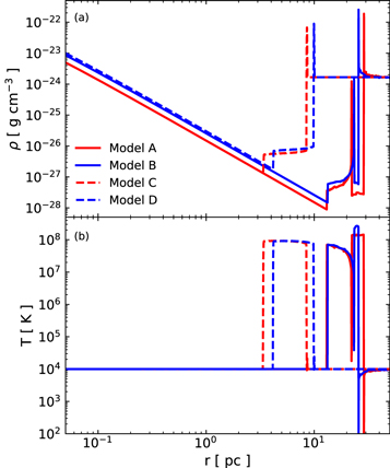
Figure 1. CSM models for a Type Ib/c SNR. Panel (a) shows the gas density as a function of radius, and panel (b) shows the gas temperature. The red (blue) solid line corresponds to the low (high) progenitor mass case. The dashed lines show the results from models for which the mass loss in the MS phase is not considered for comparison.
Download figure:
Standard image High-resolution imageFrom the results of models A and B, we can see that the CSM structure can be broken into five characteristic regions from the outer to inner radii: (i) uniform ISM, (ii) MS shell, (iii) MS bubble, (iv) W-R shell, and (v) W-R wind. The formation mechanism and features of the MS shell and MS bubble have been explained in detail in YLM21. Because the RLOF wind is characterized by a high mass-loss rate but slow velocity and a short time period, a dense (ρ ≥ 10−20 g cm−3) and compact (r ≤ 0.1 pc) structure with a power-law profile in density is formed. On the other hand, the subsequent W-R wind has a higher velocity and longer time duration than that in the RLOF phase. The fast W-R wind hence sweeps up all of the above structures created by previous phases of mass loss and creates a W-R shell at r ∼ 20 pc. This result implies that the more compact structures in the CSM created before the W-R phase are most probably washed away by the subsequent W-R wind and accumulate onto the dense W-R shell. This can also be seen in the two extra models (the βacc = 1 model and the MZAMS = 30 M⊙ single-star model) to be discussed in the Appendix. The differences in the CSM structure between models A and B are coming from the slight difference in the mass-loss rate and time duration in each pre-SN evolution phase, which leads model B to have the MS shell shifted inward and the W-R shell shifted outward, and the size of the MS bubble is reduced compared to model A.
On the other hand, because models C and D do not include the mass loss in the MS phase intentionally, the CSM structures in these models are relatively simple and can be divided into three main regions: (i) uniform ISM, (ii) W-R shell, and (iii) W-R wind. One unique feature of these models is that the W-R shell is located at a small radius r ∼ 10 pc. In these models, the W-R wind first sweeps up the dense CSM material from the RLOF phase (whose structures are almost identical to those of models A and B), beyond which the CSM density is higher than models A and B because a tenuous MS bubble is absent without the mass loss in the MS phase taken into account. The formation of the W-R shell thus happens in a shorter timescale than models A and B since the expanding W-R wind cavity is sweeping up the ISM material in the downstream, which has a much higher density than the tenuous MS bubble. The rapidly accumulating mass in the W-R shell leads to a stronger deceleration of the cavity expansion and hence a smaller cavity size prior to core collapse. There are no drastic differences between models C and D. Overall, the (non)existence of the MS mass-loss phase gives rise to the most significant variation in the hydrodynamic structure of the CSM among the models considered in this work.
In the next step, we employ these results as the initial conditions for our simulations of the subsequent SNR evolution after explosion. We note that we do not consider the effect of metallicity in the wind models and the SNR simulations, and we assume a solar abundance for simplicity. We will discuss this treatment in Section 4.
3. Results
Equipped by the CSM models described in Section 2.2, we next calculate the hydrodynamic evolution of a Type Ib/c SNR up to an age of 104 yr, and the nonthermal emissions resulted from the interaction of the SNR blast wave with the CSM environments.
3.1. Hydrodynamics
Figure 2 shows the time evolution of the SNR radius Rsk (top panel), shock velocity Vsk (middle panel), and the magnetic field B(x) at the shock position (bottom panel) for each model. Similar to YLM21, we also plot the results from a Type Ia SNR model for comparison (see YL19 and YLM21 for details). Observational data of selected core-collapse SNRs are also overlaid as black data points. These SNRs are chosen from the γ-ray source catalog of Fermi (Acero et al. 2016) and H.E.S.S. (HESS Collaboration et al. 2018a), and the exact values and references can be found in YL19.
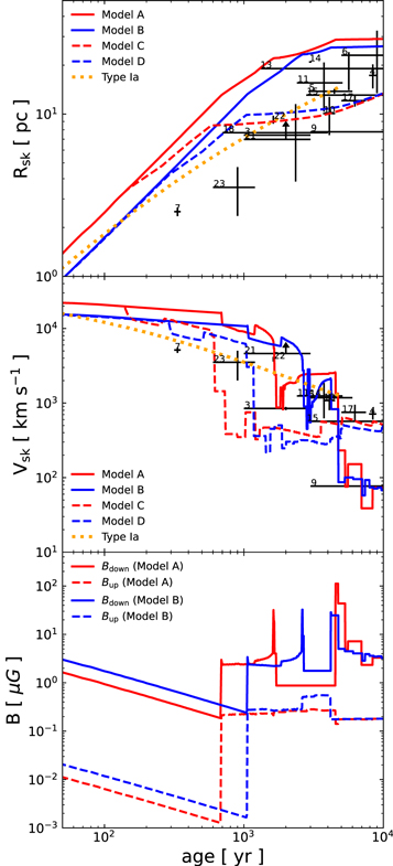
Figure 2. The hydrodynamic evolution of a Type Ib/c SNR. The top panel shows the time evolution of the forward shock radius, the middle panel shows the shock velocity as a function of SNR age, and the bottom panel shows the magnetic field at the immediate upstream and downstream of the shock. The line formats in the top and middle panels are the same as in Figure. 1. The orange dotted lines are taken from model A2 in YL19 for comparison (see text). Actual observational data of selected core-collapse SNRs are overlaid, for which the references can be also found in YL19. In the bottom panel, the red (blue) line shows the magnetic field strengths near the forward shock from model A (B). The solid (dashed) lines represent values measured at the immediate downstream (upstream) of the forward shock.
Download figure:
Standard image High-resolution imageWe first look at the results of models A (red solid line) and B (blue solid line) in the top and middle panels. In the early phase (t ≤ 1000 yr), the SNR forward shock freely expands into the tenuous unshocked W-R wind with a velocity ∼10,000 km s−1. Afterward, at an age of 1000 yr ≤ t ≤ 5000 yr, the SNR blast wave collides with the W-R shell, and the shock speed decreases to ≤1000 km s−1. The shock eventually breaks out from the W-R shell into the low-density hot MS bubble, and the shock velocity is restored to ∼2000 km s−1. In the late phase (t ≥ 5000 yr), the blast wave hits a dense wall at the MS shell and decelerates to ≤100 km s−1. As the shock sweeps up the large amount of gas contained inside the MS shell, the SNR makes a transition to its radiative phase and slowly expands into the ISM region after the shock breaks out from the MS shell. The differences between these models are mainly in the timings of transition into each dynamical phase as stated above, which in turn originate from the differences in the mass-loss rates and durations in each pre-SN evolutionary phase, as well as the ejecta mass.
From models C (red dashed line) and D (blue dashed line) in the top and middle panels, we find that the evolution in the early phase is similar to models A and B as the SNR expands into the unshocked W-R wind until it hits the termination shock and starts decelerating at an age ∼ 100 yr. Afterward, the shock collides with the dense W-R shell and slows down to a velocity of the order of 100 km s−1 at an age of around 1000 yr. As this happens, the SNR again sweeps up a large amount of gas inside the W-R shell and enters the radiative phase. When the radiative shock runs into the ISM region, the expanding hot SN ejecta heated by the reverse shock pushes the cold dense shell formed behind the radiative forward shock outward, causing the forward shock velocity to oscillate (see, e.g., Lee et al. 2015). The differences between these models are the same as what we have described above. From these results, we can see that the (non)existence of an MS bubble critically affects the dynamical evolution of a Type Ib/c SNR.
In the bottom panel, we can see that the magnetic field strengths at the immediate downstream of the shock (solid lines) are amplified from those in the upstream (dashed lines). Their evolution reflects closely the CSM structure and the shock velocity, which are critical parameters for the particle acceleration efficiency and therefore the strength of the CR-driven magnetic turbulence.
3.2. Nonthermal Emissions
Figure 3 shows the light curves of the 1 GHz radio continuum (panel (a)) and γ-ray emissions in the 1–100 GeV band (panel (b)) and the 1–10 TeV band (panel (c)). 3 The line formats and colors are the same as in Figure 2. The contributions from IC and π0 decay are independently plotted in Figure 4. The corresponding spectral energy distribution (SED) of each model is plotted in Figure 5 at four characteristic ages from left to right, which is explicitly indicated in the upper right corner of each panel.
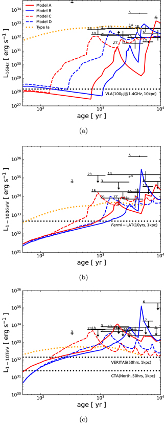
Figure 3. Light curves of the 1 GHz radio continuum (panel (a)) and γ-ray emissions integrated over the 1–100 GeV band (panel (b)) and the 1–10 TeV band (panel (c)) are shown. The line formats are the same as in Figure 2. The detection limits of VLA in panel (a), Fermi-LAT in panel (b), and VERITAS and CTA in panel (c) are plotted with black dotted lines. The results from multiwavelength observations of selected SNRs as shown in Figure 2 are also overlaid.
Download figure:
Standard image High-resolution image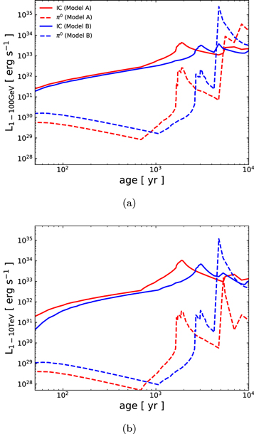
Figure 4. Same as panels (b) and (c) of Figure 3, but the contribution from each emission component is shown separately. The solid (dashed) line shows the IC (π0 decay) component, and the red (blue) color represents the results from model A (B).
Download figure:
Standard image High-resolution image
Figure 5. Broadband SED from a Type Ib/c SNR with different progenitor masses and CSM models (top to bottom) and at different ages (left to right). The exact age is shown in each panel in the upper right corner. The emission components correspond to synchrotron (blue solid), IC (magenta dashed), nonthermal bremsstrahlung (green dotted–dashed), and π0 decay (red dotted). The distance from a source is assumed to be 1 kpc.
Download figure:
Standard image High-resolution imageFrom the results of models A and B, we can observe that both the GeV and TeV γ-ray luminosities gradually increase with time, while the radio counterpart decreases during the first 1000 yr. This can be understood as follows. The dominant emission mechanism for the radio emission is synchrotron radiation, while that for the γ-rays is IC for both the GeV and TeV bands (see Figure 4 and the left panels of Figure 5). The synchrotron emissivity is proportional to both the total number of the nonthermal electrons and the square of the downstream magnetic field strength. While the wind density drops with radius as r−2 so that the injection rate becomes smaller with time, the number of accelerated electrons integrated over the volume of the SNR does increase with time as they are advected and accumulate in the downstream. The magnetic field strength immediately upstream from the shock is proportional to r−1 from the density structure, and the field strength behind the shock further decreases from adiabatic expansion and flux conservation as the shocked gas advects downstream, assuming that the magnetic fields are frozen in the shocked plasma. The overall synchrotron flux hence decreases with the expansion of the SNR. On the other hand, the IC emissivity is proportional to the product of the number of accelerated electrons and the energy density of the target photon field. Because the CMB is assumed as the photon target of IC in this work, which is constant in space, IC flux increases with time as the shock keeps accelerating electrons from the inflowing wind material.
After that, as the shock approaches the W-R shell, the luminosities in both radio and γ-rays increase with time and reach their first maxima at ∼2000–3000 yr. Until ∼4000–5000 yr, the SNR expands and breaks out into the tenuous MS bubble, and the nonthermal emission suffers a decay of 1–2 orders of magnitude from the rapid adiabatic loss, but this declination does not make the SNR undetectable by current and future instruments because the spatial extent of the MS bubble is compact as we have already explained in Section 2.2. Finally, the SNR collides with the dense MS shell and becomes bright again in all wavelengths. Once the shock enters the ISM region, it becomes hard for the shock to accelerate particles efficiently anymore owing to its low velocity, and the luminosities gradually decrease with time via adiabatic loss again.
As mentioned in Section 2.2, the W-R shells in models C and D are located at smaller radii than those in models A and B (see Figure 1 again), so that the luminosities begin to rise earlier from a few hundred years and reach maximum brightness at around 1000 yr. Until 10,000 yr, the luminosities stay at more or less the same level except for slight oscillations originating from the velocity fluctuation of the radiative shock as seen in Figure 2.
From the SED in Figure 5, we can also see a steepening of the π0 decay spectra in all models, which comes from the steepening of the underlying proton spectrum. The power-law index of the proton spectrum is roughly obtained as  , where Stot is the effective compression ratio (e.g., Caprioli et al. 2009), which is determined by the difference between the shock velocity and the velocity of the magnetic scattering centers. In situations where MFA is efficient, the effective compression ratio can become smaller than 4 and the resulting proton spectra hence steepen. As a result, when π0 decay is the dominant emission channel in the late evolutionary phase, the total γ-ray spectrum is characterized by a soft spectrum.
We note that the luminosity of the "Type Ia" model referenced here is relatively large compared to the Type Ib/c models, especially in the early phase. This is stemming from differences in the assumed DSA injection rate χinj and the surrounding ISM/CSM environment. The injection rate χinj determines the amount of particles injected into the acceleration process and the resulting acceleration efficiency (see, e.g., Blasi 2004; Blasi et al. 2005). Here we have adopted χinj = 3.6 for the Type Ia model and χinj = 3.75 for the Type Ib/c models based on YL19. More importantly, according to our CSM models, Type Ib/c SNRs expand into a tenuous wind cavity, whereas the Type Ia model adopts a uniform ISM-like environment with nISM = 0.1 cm−3 as in YL19. While the absolute luminosities do depend on the DSA parameters, which should be constrained by observation data of individual SNRs, our results show that the light curve of a Type Ia SNR evolving in a more or less uniform ISM is expected to be much flatter and uncharacteristic compared to the remnants of Type Ib/c SNe, for which the latter heavily anchors to the highly inhomogeneous structure of the CSM environment and hence the progenitor mass-loss history.
We can now assess the observational detectability of a Type Ib/c SNR based on our models. The sensitivities of various instruments are plotted in all panels in Figure 3 with black dotted lines. For the radio band, we compare the detection limit of the Very Large Array (VLA) with our models. The sensitivity for a targeted observation of objects like radio galaxies and active galactic nuclei is ∼100 μJy at 1.4 GHz (e.g., Schinnerer et al. 2004; Simpson et al. 2012), and the lower limit from a source at a distance of 10 kpc therefore corresponds to ∼2 × 1028 erg s−1. We note that nontargeted sky surveys have much shallower sensitivities, but this does not affect the following discussion and our main conclusion. We use the sensitivity of the Fermi Large Area Telescope (Fermi-LAT) for the GeV γ-rays and VERITAS (Very Energetic Radiation Imaging Telescope Array System) and the Cherenkov Telescope Array (CTA) for TeV γ-rays. Based on 10 yr of survey data 4 (see, for details, Abdollahi et al. 2020; Ballet et al. 2020), the flux sensitivity of Fermi-LAT in the 1–100 GeV range is ∼2 × 10⁻¹² erg cm−2 s−1, which corresponds to a luminosity ∼4.8 × 1032 erg s−1 for a γ-ray source at 1 kpc. Those of VERITAS and the northern telescopes of CTA in the 1–10 TeV band with an observation time of 50 hr are ∼6 × 10⁻¹³ erg cm−2 s−1 and ∼10−13 erg cm−2 s−1, respectively. 5 For a source at a distance of 1 kpc, the detection limits are ∼1.4 × 1032 erg s−1 and ∼2.4 × 1031 erg s−1. In this calculation, we do not take other effects like interstellar absorption into account.
Our results show that Type Ib/c SNRs are most probably too faint to be observed in radio and GeV γ-rays in the first 1000 yr after explosion, although they can potentially be detected as a TeV-bright SNR in the CTA era if they are close by (≲1 kpc). On the other hand, the SNRs are bright enough to be detectable in all wavelengths from 1000 to 10,000 yr after the blast wave has swept through the low-density W-R wind and starts to interact with the denser CSM beyond the W-R wind. We can conclude that Type Ib/c SNRs are very likely to experience a "resurrection" in nonthermal brightness, meaning that they are too dark to be observable in the first 1000 yr but rebrighten significantly afterward until 10,000 yr. If the MS bubble does not exist, even younger SNRs can become detectable. However, we note that while the occurrence of the "resurrection" is a robust prediction of our models, its exact timing depends on various additional factors that we have not fully explored in our parameter space, such as the nature of the progenitors, including their ZAMS masses and mass-loss rates, as well as the surrounding ambient environment in which they evolve (e.g., in or near a giant molecular cloud).
4. A Comparison with Type II SNRs
4.1. Light Curves
The present results as complemented with the results of YLM21 provide a new picture of SNR evolution highlighted by the difference between Type II and Ib/c SNRs, which is directly linked to their progenitor evolution. Figure 6 compares the model light curves of Type II SNRs from YLM21 and Type Ib/c SNRs presented in this study. The red lines correspond to Type II remnants (see models A and B in YLM21) and the blue lines to Type Ib/c objects (this work). The solid and dashed lines represent models with MZAMS = 12 and 18 M⊙, respectively. In YLM21, the authors proposed that Type II SNRs are very likely to experience a "dark age" in which the SNRs become too faint to detect in multiwavelength for a prolonged period of time. Meanwhile, this work suggests that Type Ib/c SNRs can experience a "resurrection" after a certain age. Combining these results, and for a fixed condition of the ambient ISM, it can be found that Type II SNRs tend to be bright when Type Ib/c ones are faint, and vice versa. These results suggest a profound implication that there may exist an observational bias in the detected SNR population, in which there is a correlation between the SNR ages and their originating SN types and progenitor natures, thus providing an additional tool for the back-engineering of the observed SNRs and linking them to their progenitor stars and SN explosions.

Figure 6. Comparison of Type II SNRs (red lines; YLM21) and Type Ib/c SNRs (blue lines; this work). Solid lines plot the results of the MZAMS = 12 M⊙ model, and dashed lines show those of the 18 M⊙ model for both colors. The detection limits of various detectors are also plotted with black lines as shown in Figure 3.
Download figure:
Standard image High-resolution imageHowever, the determination of SNR age (and distance for that matter) is usually a nontrivial task. Except when an SNR is identified with historical SNe like Tycho's and Kepler's SNR, the age is generally obtained from the sigma-D relation (e.g., Poveda & Woltjer 1968; Clark & Caswell 1976; Case & Bhattacharya 1998), which can involve large uncertainties. Suzuki et al. (2020) show that the dynamical age from fitting the apparent diameter with the Sedov solution provides good agreement with the plasma age inferred from X-ray observations of the nonequilibrium ionization plasma in several SNRs (see their Figure 9). Further improvements in the accuracy of age determination through multiwavelength observations are hence critical for linking any observed core-collapse SNR to its progenitor origin and SN type.
4.2. Spectral Properties
In addition, we found that our results well reproduce the observations of several γ-ray-bright SNRs as well in terms of their spectral properties. As mentioned above, Type II SNRs are bright in γ-rays in their early evolutionary phase. As shown by Figure 4 in YLM21, their dominant γ-ray emission process is via π0 decay. On the other hand, Type Ib/c SNRs are γ-ray bright in ages when their Type II counterparts tend to become faint, with the primary emission component being IC emission (see top panels of Figure 5). From these results, one can expect that the γ-ray spectrum of an SNR is characterized by (i) a flat spectrum produced by π0 decay at a very young age (≤1000 yr old) as dominated by a Type II origin, (ii) a hard spectrum from IC emission at intermediate ages (≤5000 yr old) with a Type Ib/c origin, and (iii) a soft spectrum at older ages (≥10,000 yr old) independent of SN type (i.e., a mixture of Type II and Ib/c SNRs) as the shock has collided with the dense MS shell and decelerates, with π0 decay being the dominant emission component. In panel (a) of Figure 7, we plot our simulation results for the SEDs in the sub-GeV to 100 TeV band of Type II SNRs and Type Ib/c ones at the indicated characteristic ages. Meanwhile, panel (b) shows the observed γ-ray SEDs of a few core-collapse SNRs. Indeed, we can see that very young objects like Cas A do exhibit a relatively flat spectrum (Acciari et al. 2010; Yuan et al. 2013; Ahnen et al. 2017; Abeysekara et al. 2020), while SNRs a few × 103 yr old like RX J1713.7−3946 (Abdo et al. 2011; HESS Collaboration et al. 2018b), Vela Jr (Tanaka et al. 2011; HESS Collaboration et al. 2018c), and G150.3+4.5 (Devin et al. 2020) show harder spectra, and the more evolved middle-aged SNRs like IC 443 and W44 (Ackermann et al. 2013) typically show very soft spectra. While this general agreement does not necessarily imply that the picture above is applicable for every single individual object, our results imply in general a strong correlation of the γ-ray spectral properties of an SNR with its progenitor nature and hence the mass-loss history and CSM structure.
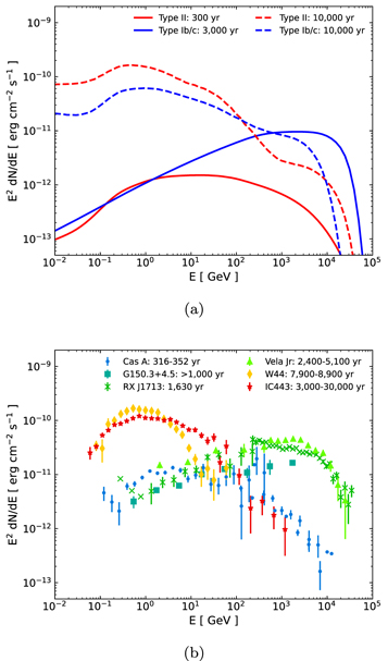
Figure 7. (a) Simulated γ-ray SED from this work and YLM21. Red lines show the results of model A in YLM21 at 300 yr (solid) and 10,000 yr (dashed), and blue ones correspond to those of model A in this work at 3000 yr (solid) and 10,000 yr (dashed). (b) SEDs of several core-collapse SNRs. References of each SNR: Cas A (Ahnen et al. 2017; Abeysekara et al. 2020), G150.3+4.5 (Devin et al. 2020), RX J1713 (HESS Collaboration et al. 2018b), Vela Jr (Tanaka et al. 2011; HESS Collaboration et al. 2018c), W44 (Ackermann et al. 2013), and IC 443 (Albert et al. 2007; Ackermann et al. 2013). The values of age estimations are taken from SNRcat (Ferrand & Safi-Harb 2012, and http://www.physics.umanitoba.ca/snr/SNRcat/).
Download figure:
Standard image High-resolution imageWe emphasize that this transition of the SED properties is expected only when we consider the mass-loss histories of the progenitors. For example, YL19 also attempted to calculate the time evolution of core-collapse SNRs with a method similar to this work, but they assumed that the SNRs are embedded within a simple power-law CSM (ρ ∝ r−2) without considering the pre-SN mass-loss history. Their more simplistic models did not predict such an SED transition described above regardless of the choice of parameters such as the mass-loss rate, whereas the transition emerges naturally in this work and YLM21 by using more self-consistent CSM models linked to the evolution of the progenitor stars. Moreover, a mixture of SN types is found to play an important role as well.
4.3. Additional Remarks
One caveat is that our simulation is one-dimensional and we assume that the SN progenitors evolve into an ISM with a fixed density of 1 cm−3. However, many core-collapse SNRs are known to have asymmetrical morphologies, and some of them are known to be interacting with high-density materials like molecular clouds as mentioned above. Hence, we do not expect that our results can be applied to explain detailed properties of every individual SNR. The investigation of multidimensional effects and the diversity of the surrounding ISM is postponed to a future work. Nonetheless, we believe that our one-dimensional but sophisticated evolution models succeed in capturing a big picture of how the pre-SN evolution of the progenitors, which spans millions of years, can be linked to the observational properties (nonthermal emission in particular for this work) of their SNRs thousands of years after the explosion.
Another additional factor that we have not explored yet is the effect of a nonsolar metallicity. We assume a solar abundance throughout our simulation box, while we expect that the W-R wind should possess a metal-rich composition such as helium and/or carbon−oxygen. However, we note that this does not affect our main results because the dominant nonthermal emission mechanisms while the blast wave is inside the W-R wind are from synchrotron in radio and IC in GeV–TeV band, respectively, for which the effect from an altered metallicity is mainly on the free electron number density. We can estimate that the change of the density in a helium-rich environment is only about a factor different from that in an environment with a solar-like abundance. This error is much smaller than the uncertainties from poorly constrained parameters such as the mass-loss properties, distance, and so on. We hence ignore the metallicity for our calculations of nonthermal emissions here as a secondary effect. A future follow-up study will include other processes such as heavy ion acceleration and escape in the stellar wind as well (Biermann et al. 2010; Ohira & Ioka 2011; Aguilar et al. 2015a, 2015b, 2017) and investigate their effects on the resultant nonthermal emission properties.
Finally, it is illustrative to discuss other possible subtypes of SNRs beyond what we have modeled so far. For example, almost 10% of all core-collapse SNe are classified as Type IIb (Smith et al. 2011), of which the representative remnant objects include the Galactic SNR Cassiopeia A (Borkowski et al. 1996; Krause et al. 2008). Their progenitors are believed to be helium stars embraced by a thin hydrogen envelope that is not completely stripped off by the binary interaction and stellar winds. They show a diversity in the CSM density, but it is generally larger than the W-R wind case and close to the RSG wind. As such, we expect that Type IIb SNRs will evolve in a similar manner to Type II SNRs. In addition, the diversity in the CSM density and thus in the final mass-loss rate is suggested to be linked to the timing of the binary interaction (Maeda et al. 2015), which may reflect expected diversity in the initial binary configuration leading to SNe IIb (Ouchi & Maeda 2017). Therefore, theoretical investigation adopting realistic mass-loss history for SNe IIb will provide an interesting possibility to further constrain the details of the stellar evolution scenarios and roles of the binary interaction toward SNe. An expansion of our work to model other possible types of SNRs will be found in a follow-up paper.
5. Conclusion
Nonthermal emission from various types of SNRs is an effective probe of their surrounding environment and hence the nature and evolution of their progenitor stars. Following the method of YLM21, who focused on Type II SNRs, we have conducted simulations of the long-term evolution of Type Ib/c SNRs interacting with their CSM in this work, taking into account the mass-loss history of their progenitors. The nonthermal emissions produced by the interactions between the accelerated CRs and the surrounding environment are presented.
We show that the nonthermal emissions from Type Ib/c SNRs are faint and below the sensitivities of current and near-future detectors in the early phase when the SNR blast wave is inside the unshocked W-R wind region (t ≤ 1000 yr), except if the source is extremely close (d ≤ 1 kpc) and the TeV emission can be potentially picked up by future observatories such as CTA. These objects are also predicted to be nonthermally bright after the SNR shock has begun to penetrate through the W-R wind shell (t ≥ 1000 yr). As the SNR shock passes through the dense shell at around 2000–3000 yr, the brightness of SNRs decreases gradually owing to the weakening of the shock and fast adiabatic cooling in the hot compact MS bubble until 5000 yr. Finally, they collide with the dense MS shell and rebrighten again, but they gradually lose their punches once more because of the rapid deceleration of the shock into the radiative phase. We conclude that the nonthermal emission from most Type Ib/c SNRs should experience a "resurrection" at some point (∼1000 yr for a typical ambient ISM density of n = 1 cm−3) for progenitors with ZAMS mass MZAMS ≤ 18 M⊙. While the exact values of the timescales mentioned above are dependent on the (non)existence of the MS bubble, the ejecta mass, the wind and ISM properties, and so on, our conclusion on the predicted general evolution of a Type Ib/c SNR stays robust because it is independent of any fine-tuning of parameters.
We have also compared the results in this work to a previous study on Type II SNRs as reported in YLM21. We show that while Type II SNRs are expected to be bright in the first 1000 yr or so but faint afterward for a few × 103 yr in both radio and γ-rays, Type Ib/c SNRs are showing opposite evolution characteristics, i.e., they are predicted to be dark in the early phase but rebrighten after an age of about 1000 yr, assuming an n = 1 cm−3 ISM density. This contrasting behavior leads to an evolutionary picture for the SNR population that is found to be compatible with the γ-ray observation of core-collapse SNRs, in particular the observed broadband spectral properties against the SNR ages, which cannot be reproduced by simplistic models without considering the mass-loss histories of the SN progenitors. Another profound implication from our results is that there is a possible observational bias in the current and future SNR observations, i.e., the SN type and progenitor origin of an observed SNR are correlated to its age or evolutionary phase. By the inclusion of other SN subtypes (probably including the different kinds of Type Ia SNRs as well), and as further observational constraints become available in the future, we plan to expand our work to provide a more complete description of the SNR population as a whole.
H.Y. acknowledges support by JSPS Fellows grant No. JP20J10300. S.-H.L. acknowledges support by JSPS grant No. JP19K03913 and the World Premier International Research Center Initiative (WPI), MEXT, Japan. K.M. acknowledges support from JSPS KAKENHI grants JP18H05223, JP20H04737, and JP20H00174.
Appendix A: Additional Models
As mentioned in Section 2.2, we have included two additional models here for reference: (i) a model in which all the matter stripped off by RLOF is accreted onto the secondary star (i.e., βacc = 1; hereafter model E), and (ii) a model in which a massive star with MZAMS = 30 M⊙ evolves as a single star without binary interactions (hereafter model F). Figure A1 shows the CSM density profiles for the two models, and the model parameters are summarized in Table A1. Figure A2 plots the time evolution of their nonthermal radio and γ-ray luminosities. The red and blue solid lines correspond to models E and F, respectively, and we also overplot the results of the fiducial model B as a comparison.
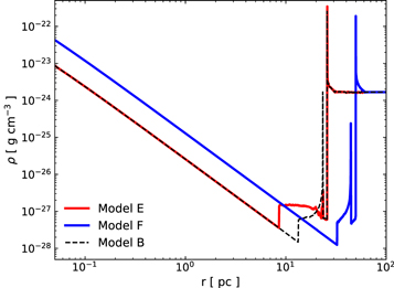
Figure A1. Radial density profiles of the CSM for the two additional models. The red solid line corresponds to model E (βacc = 1), and the blue solid line corresponds to model F (MZAMS = 30 M⊙). The black dashed line shows the result of model B for comparison.
Download figure:
Standard image High-resolution image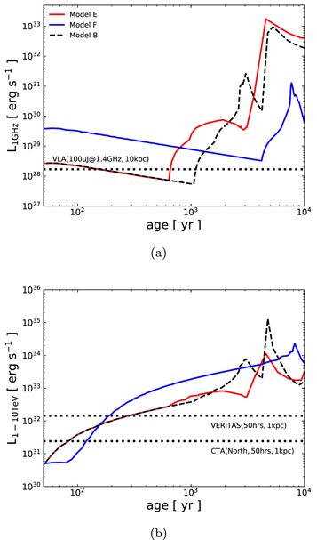
Figure A2. Light curves in (a) 1 GHz radio continuum and (b) 1–10 TeV band for the additional models. The line formats are the same as in Figure A1, and the detection limits as shown in Figure 3 are also shown.
Download figure:
Standard image High-resolution image
Table A1. Parameters of Two Additional Models
| Model | MZAMS | Wind Phases |

| Vw | Mw | τphase | Mej |
|---|---|---|---|---|---|---|---|
| (M⊙) | (M⊙ yr−1) | (km s−1) | (M⊙) | (yr) | (M⊙) | ||
| E | 18 | MS | 6.0 × 10⁻⁷ | 2000 | 0.3 | 5.0 × 10⁶ | |
| RLOF | 0.0 | 10 | 0.0 | 1.0 × 10⁴ | |||
| W-R | 1.0 × 10⁻⁵ | 2000 | 1.0 | 1.0 × 10⁵ | 2.5 | ||
| F | 30 | MS | 5.0 × 10⁻⁷ | 2000 | 2.0 | 4.0 × 10⁶ | |
| RSG | 5.0 × 10⁻⁵ | 10 | 18.0 | 3.6 × 10⁵ | |||
| W-R | 5.0 × 10⁻⁵ | 2000 | 5.0 | 1.0 × 10⁵ | 3.5 | ||
Note. The wind parameters and ejecta properties of two additional models are shown. Other details are as written in the footnote of Table 1.
Download table as: ASCIITypeset image
A.1. Model E
From Figure A1, we can see that there are two major differences between models E and B. One is that the density in the W-R shell is smaller by more than two orders of magnitude in model E; the other is that the termination shock is sitting at a more inner region in the W-R wind. These are caused by their differences in the CSM formation history. As the matter stripped off from the progenitor by RLOF in model E is accreting onto the secondary star without contributing to the CSM gas distribution, the mass swept by the subsequent W-R wind is much smaller than in model B, and the W-R shell contains a much smaller mass. This also leads to a faster expansion of the W-R wind toward the outlying ISM, resulting in the termination shock propagating further inward against the outgoing unshocked W-R wind in the last 105 yr.
These differences in the CSM structure are directly reflected in the light curves shown in Figure A2. In model E, the SNR shock collides with the termination shock at an earlier time, and the luminosities in both energy bands start to rise from ∼600 yr. The luminosities reach their maximum values at ∼2000 yr but are smaller than in model B because the mass inside the W-R shell is much smaller. This implies that if βacc ≃ 1, it becomes more difficult to detect Type Ib/c SNRs, especially in γ-rays.
A.2. Model F
One of the distinctive features of model F is a higher mass-loss rate in each wind phase as shown in Table A1, which is reflected by the higher density in the wind in Figure A1. Another difference is that the main mass-stripping mechanism is not via binary interaction but the RSG wind. Nevertheless, the CSM structures of models B and F are found to be qualitatively similar to each other, except that it is more spread out in radius for model F. As explained in Section 2.2, the high-velocity wind from the W-R star sweeps the RSG wind up quickly, forming a similar CSM structure to that in model B. The W-R wind in model F has a high ram pressure from the higher mass-loss rate; therefore, the wind shell is formed at a more outer region.
From Figure A2, we find that these types of SNRs expand into the high-density wind region for about 4000 yr, and they are brighter in both radio and γ-rays than SNRs with a lower-mass progenitor in binaries for the first 1000 yr or so. They do, however, become relatively faint in radio afterward, during 1000–4000 yr, due to the fact that the SNR shock is still interacting with the unshocked power-law W-R wind, while in model B it has already collided with the dense W-R shell. From this point on, the light curves exhibit a similar behavior to model B. This result suggests that a detection of bright nonthermal emission from a very young Type Ib/c SNR (e.g., a couple hundred years old) may imply a high-mass single star for the progenitor, but most probably it will be difficult to distinguish between a single star and binary origin solely from the observed nonthermal emission properties because the details in the pre-SN mass-loss history are almost washed away in the emergent CSM structure by the fast W-R wind prior to explosion.
Footnotes
- 3
We note that X-ray emission is also important for deciphering the properties of SNRs. X-rays from SNRs are produced by not only synchrotron radiation but also thermal components including bremsstrahlung, various continua, and line emission from the hot plasma confined between the forward and reverse shock. By focusing on the nonthermal components in this work, we postpone the presentation of light curves in the X-ray bands to a future work in which a proper implementation of the thermal emission will be included.
- 4
- 5
VERITAS specifications from https://veritas.sao.arizona.edu/about-veritas/veritas-specifications, and CTA performance from https://www.cta-observatory.org/science/ctao-performance/.