


Abstract
We present observations during the interval 2006–2014 of 27 day and 13.5 day periodic oscillations in the ionospheric sporadic E (Es) layer. This is a thin, dense layer composed of metallic ions in the Earth's upper atmosphere between 90 and 130 km. Lomb–Scargle spectral and wavelet analyses reveal that these pronounced periodicities observed from ground-based ionosondes and GPS/GNSS radio occultations are associated with high-speed solar winds generated from persistent coronal holes on successive 27 day solar rotations. The 27 day and 13.5 day oscillations in the Es layers are dependent on latitude, showing a higher magnitude of periodicities at low latitudes between 0° and 15° and at high latitudes between 45° and 90° (10%–14%) than those at midlatitudes between 15° and 45° (4%–10%). The 27 day and 13.5 day oscillations in the high-latitude Es layers correlate well with the geomagnetic activity Dst and Ap indices, and these periodic oscillations become more significant at the solar maximum (2000–2003 and 2011–2014) than at the solar minimum.
Export citation and abstract BibTeX RIS

Original content from this work may be used under the terms of the Creative Commons Attribution 4.0 licence. Any further distribution of this work must maintain attribution to the author(s) and the title of the work, journal citation and DOI.
1. Introduction
Variability in near-Earth interplanetary and terrestrial parameters is affected by the Sun. The Earth's upper atmosphere and ionosphere are strongly modulated by solar activity, which exhibits 11 yr, annual, and interannual (semiannual, seasonal, 27 day, and diurnal) periods. Many studies have identified clear solar–terrestrial connections in meteorological (Schlegel et al. 2001; Scott et al. 2014a; Owens et al. 2014; Maycock et al. 2015), ionospheric (Rishbeth & Mendillo 2001; Scott et al. 2014b; Lockwood et al. 2016b), auroral (Silverman 1992; Vázquez et al. 2006; Xing et al. 2012; Zhang et al. 2020), geomagnetic (Svalgaard & Cliver 2010; Chi et al. 2016; Owens et al. 2016a; Lockwood et al. 2019b), magnetospheric (Petrinec et al. 1991; Lockwood et al. 2019a, 2020), and cosmogenic isotope (McCracken et al. 2004; Lockwood 2006; McCracken & Beer 2007; Owens et al. 2016b) observations.
The 11 yr solar cycle is one of the most prominent variations in the solar wind and heliospheric magnetic field (Owens et al. 2018). Many previous studies have concentrated on the response of the F-layer and topside ionosphere to the 11 yr solar cycle (Allen 1948; Cliver et al. 1998). Rishbeth & Mendillo (2001) found that the solar ionizing radiation, the solar wind/geomagnetic activity, and the meteorological effects are the likely causes of F2-layer variability. Spectral analyses of the long-term changes in the critical frequencies of F2 layers (foF2) and total electron content (TEC) confirm a dominant 11 yr solar cycle variation (Khaitov et al. 2014; Tang et al. 2014).
The approximately 27 day synodic rotation period of the Sun is one prominent short-term periodic variation in the solar wind and near-Earth interplanetary parameters (Beck 2000). The recurrence of geomagnetic activity is attributed to the passage of high-speed solar winds at Earth, which originate from persistent coronal holes at low heliographic latitudes on successive solar rotations (Chi et al. 2018). Lei et al. (2008b) reported the ionospheric response of periodic oscillations in global mean TEC to the earthward high-speed streams of solar wind that arise from such coronal holes. The 9 day and 13.5 day periodicities in the F2 peak electron densities (NmF2) are associated with the 27 day solar-rotation period (Wang et al. 2011). The 9 day periodic oscillations were also found in the upper atmospheric densities caused by a triad of solar coronal holes that occurred roughly 120° apart in solar longitude (Lei et al. 2008a; Yi et al. 2017).
The ionospheric sporadic E (Es) layer at altitudes between 90 and 130 km is of particular interest in ionospheric investigations, because it is a thin layer composed of terrestrial metallic ions of meteoric origin near the boundary between the upper atmosphere (containing the ionosphere) and the lower neutral atmosphere (Cai et al. 2019; Yu et al. 2019a). The plasma irregularities in Es layers can significantly affect signals from the Global Positioning System (GPS)/Global Navigation Satellite System (GNSS) by causing a temporary loss of phase lock between the two frequencies in use to eliminate ionospheric propagation effects (Yue et al. 2016; Yu et al. 2020). Diurnal and semidiurnal atmospheric tides are known to dominate the short-term variations in Es layers (Mathews & Bekeny 1979). Meteorological processes including mesoscale convective weather, thunderstorms, and wave activities from the troposphere can influence the short-term variations in mesospheric metallic atoms and ions (Davis & Johnson 2005; Johnson & Davis 2006; Yu et al. 2015, 2017, 2019b). In addition, planetary waves are responsible for the periodicities of 2, 5, 10, and 16 days in the Es layers (Haldoupis et al. 2004). Recent work reported a response of the mesospheric neutral metal layers to the 27 day solar rotation cycle (Wu et al. 2019). However, the relationship between the 27 day solar rotation and the short-term periodicity in the abundance of metallic ions within Es layers has not been fully explored before.
The long-term series of ionospheric data recorded at Sodankylä, Finland and Slough, UK have proved invaluable in identifying the signatures of the 27 day solar rotation in the Es layers during solar maximum and minimum periods. In this paper, the effect of the 27 day solar rotation on the terrestrial metallic ions is investigated. It is worth noting that in early studies of sporadic-E no 27 day recurrence could be detected (e.g., Wells 1946) and a great many subsequent studies of the phenomenon only looked at the means, medians, and occurrence frequencies over 27 day intervals. The correlation between the 27 day periodic oscillations in Es layers and changes in the disturbance storm time (Dst) index and the geomagnetic activity Ap index is analyzed. Based on satellite radio occultation (RO) data, the dependence of the Es formation on the solar rotation is studied, by analyzing the periodic responses of Es layers at low to high latitudes. The mechanisms involved in the formation of sporadic E layers are thought to be wind shear effects (which dominate the formation of midlatitude Es layers) and the effects of plasma instabilities accompanied by strong electric fields with intense magnetic activities (which dominate at low latitudes and at high latitudes). Understanding the influences of solar rotation on the lower ionosphere is of vital importance to the study of the solar–terrestrial connection and possible processes that enable the solar-wind energy to impact the Earth's atmospheric weather systems via the global electric circuit (Jánský et al. 2017).
2. Data Description
The ionosonde data used in this study were obtained from the UK Solar System Data Centre (UKSSDC, www.ukssdc.ac.uk) at the Rutherford Appleton Laboratory (Davis et al. 2013) and the Data Centre of the Chinese Meridian Project (Wang 2010). All the ionosonde observations were manually scaled. The UK ionospheric monitoring group has made long-term observations of the ionosphere at Slough (51.5°N, 0.6°W) in the UK from 1931 to 1995. The high-latitude ionosonde data at Sodankylä, Finland (67.4°N, 26.6°E) from 1993 to 2018 were also used to study the behavior of the Es layers in the auroral zone. A total of 16 ionosonde stations listed in Table 1 were used to investigate the global Es layers. The critical frequencies of Es layers (foEs) data were analyzed. The parameter foEs represents the peak radio frequency returned from the Es layers and it is a measure of the peak electron concentration via the relation  , where Ne
is the peak electron concentration (in m−3).
, where Ne
is the peak electron concentration (in m−3).
Table 1. Ionosonde Stations Used in the Wavelet Analysis of the Global Variations in the 27 day Oscillations in foEs
| No. | St. Code | St. Name | Lat. | Long. | Mag. Lat. | Mag. Long. | Years | 12–30 day Power | Ratio of Power |
|---|---|---|---|---|---|---|---|---|---|
| (deg) | (deg) | (deg) | (deg) | (MHz2) | (%) | ||||
| 1 | SO166 | Sodankylä | 67.40 | 26.60 | 63.90 | 119.74 | 2006–2014 | 0.30 | 8.41 |
| 2 | MH453 | Mohe | 52.00 | 122.50 | 42.10 | −167.78 | 2010–2014 | 0.15 | 6.49 |
| 3 | ML449 | Manzhouli | 49.60 | 117.50 | 39.55 | −171.82 | 2008–2014 | 0.50 | 9.14 |
| 4 | BP440 | Beijing | 40.30 | 116.20 | 30.22 | −172.56 | 2006–2014 | 0.36 | 5.48 |
| 5 | WU430 | Wuhan | 30.50 | 114.40 | 20.41 | −173.91 | 2010–2014 | 0.37 | 6.08 |
| 6 | 09429 | Chongqing | 29.50 | 106.40 | 19.36 | 178.72 | 2008–2014 | 0.55 | 4.34 |
| 7 | GU421 | Guangzhou | 23.10 | 113.40 | 13.02 | −174.70 | 2008–2014 | 0.45 | 5.67 |
| 8 | SA418 | Sanya | 18.30 | 109.40 | 8.21 | −178.45 | 2007–2014 | 0.30 | 6.65 |
| 9 | CS31K | Cocos Is | −12.20 | 96.80 | −21.91 | 168.41 | 2008–2014 | 0.19 | 13.61 |
| 10 | DW41K | Darwin | −12.45 | 130.95 | −21.51 | −155.61 | 2006–2014 | 0.20 | 11.53 |
| 11 | BR52P | Brisbane | −27.53 | 152.92 | −34.16 | −130.49 | 2006–2014 | 0.30 | 7.36 |
| 12 | CB53N | Canberra | −35.32 | 149.00 | −42.34 | −133.21 | 2006–2014 | 0.33 | 5.74 |
| 13 | HO54K | Hobart | −42.92 | 147.32 | −50.04 | −133.28 | 2006–2014 | 0.29 | 7.52 |
| 14 | GH64L | Christchurch | −43.42 | 172.34 | −46.79 | −106.08 | 2006–2011 | 0.31 | 9.01 |
| 15 | MQ55M | Macquarie Island | −54.50 | 159.00 | −59.69 | −115.72 | 2006–2013 | 0.36 | 10.10 |
| 16 | MW26P | Mawson | −67.60 | 62.90 | −73.08 | 111.63 | 2006–2014 | 0.45 | 16.24 |
Download table as: ASCIITypeset image
GNSS RO is a relatively new meteorological remote sensing technique to observe atmospheric parameters such as temperature, water vapor content, and pressure. Irregularities in the electron concentration of the intense metallic ions within Es layers can have significant effects on the amplitude and phase of GNSS RO signals. These effects on the GNSS RO signals can be exploited for ionospheric global investigations. Previous works indicate that the amplitude scintillation S4 index from RO signals can be used as a proxy for the intensity of Es layers (Arras & Wickert 2018; Resende et al. 2018; Yu et al. 2019a). The global data on critical frequencies of the Es layer (foEs) from 2006 to 2014 have been derived based on the Constellation Observing System for Meteorology, Ionosphere and Climate (COSMIC) S4max data set (Yu et al. 2019a, 2020). An advantage of the foEs data derived from the COSMIC satellites is that it enables a full global coverage of this parameter. Based on the RO data, the latitudinal variations and the global behavior of Es layers can be investigated, combined with observations from the global ground-based ionosondes.
The solar wind and geomagnetic activity are characterized by the solar wind speed, solar 10.7 cm radio flux (F10.7), and geomagnetic activity Dst and Ap indices. The solar wind observations are taken from the OMNIWeb database including those obtained by the IMP 8, Wind, and ACE spacecraft. The geomagnetic activity Ap index is provide by the UKSSDC and the Dst index is provided by the World Data Center, Kyoto, Japan.
3. Observational Results
3.1. 27 day Periodicity and Its Harmonic Oscillations in Es Layers
Figure 1(a) shows the variations in daily mean foEs values in the period 1993–2018 from the ionosonde at Sodankylä, Finland. The observed foEs shows the dominant annual and 11 yr solar cycle variations. The dominant influence on the ionosphere at periods around 27 days is the solar rotation and the corotation of long-lived (meaning lasting several solar rotations) structure in near-Earth interplanetary space and the "lighthouse" effects of similarly long-lived regions of enhanced solar irradiance at relevant wavelengths (Harrison & Lockwood 2020). The period of such variations can vary but is generally close to the Carrington rotation interval of 27.26 days (the period of rotation of the solar photosphere at 26° heliographic latitude, close to the average latitude of sunspots and active regions). The only other period close to this is the lunar orbit period, which generates the sidereal monthly tide component of period 27.55 days. Studies of the power spectra of "geomagnetic tides", caused by the solar and lunar gravitational effects on ionospheric currents, find this component to usually be undetectably small (e.g., Love & Rigler 2014), and the largest effects seen are "13 day" or "semimonthly" variations at period 27.55/2 = 13.78 days, which are strongest in the equatorial electrojet following a stratospheric warming (e.g., Park et al. 2012). Hence we here take variations seen near 27 days to be due to solar rotation. To analyze the short-term variations in Es layers related to the 27 day solar rotation cycle, a sixth-order Butterworth filter has been applied in the time series of foEs. This low-pass temporal filter can separate the long-term and short-term trends of foEs and does not change the temporal phase. The cutoff period is 60 days. The filtered foEs with periods more than 60 days is shown as a dark pink line while the raw data are shown in light pink. In this study, we concentrate on the variability in the short-term periodicities, so we subtract the filtered foEs from the raw data and obtain the residual foEs (δfoEs) with periods less than 60 days, as shown by blue lines.
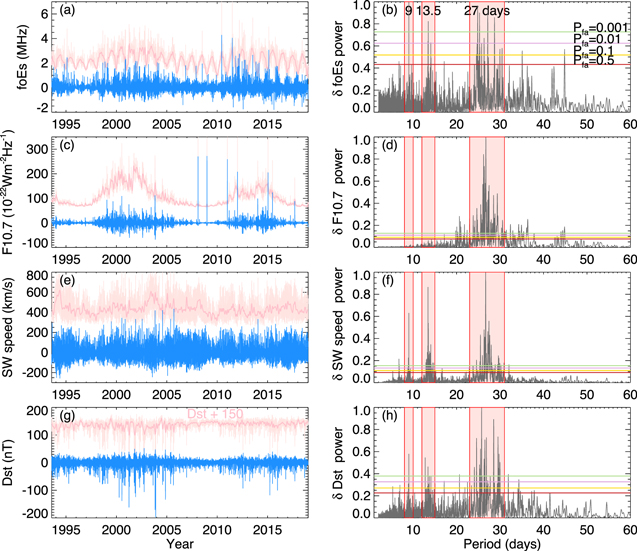
Figure 1. High-frequency fluctuations with a period band between 1 and 60 days (left panels) and the corresponding normalized Lomb–Scargle periodogram (right panels) of the daily mean foEs (MHz) from a high-latitude ionosonde at Sodankylä, Finland (67.4°N, 26.6°E), F10.7 (10−22 W m−2 Hz−1), solar wind speed (km s−1), and Dst index from 1993 to 2018. In the left panels, the blue lines represent the high-frequency fluctuations (1–60 day period), after subtracting the climatological changes with periods longer than 60 days (dark pink) from the raw data (light pink), by using a low-pass Butterworth filter of sixth order in time with a cutoff period of 60 days. The right panels are the corresponding normalized Lomb–Scargle periodograms; the predominant spectral peaks at approximately 9, 13.5, and 27 days are represented by the red shaded area. The horizontal lines represent the false-alarm probabilities of 50%, 10%, 1%, and 0.1%.
Download figure:
Standard image High-resolution imageTo study the short-term periodic oscillations in δfoEs, a Lomb–Scargle spectral analysis (Lomb 1976; Scargle 1982) was conducted. Figure 1(b) shows the normalized Lomb–Scargle periodogram, while the horizontal lines correspond to false-alarm probabilities of 50%, 10%, 1%, and 0.1%. The predominant spectral peaks in the short-term changes of foEs are at periods of approximately 27, 13.5, and 9 days. The 27 day periodicity can also be observed in the daily F10.7 (Figures 1(c) and (d)), the solar wind speed (Figures 1(e) and (f)), and the Dst index (Figures 1(g) and (h)), but the 13.5 day and 9 day periodicities were not found in the F10.7 corresponding to the second and third harmonics of the 27 day solar rotation cycle. Recurrent fast solar wind streams, known as corotating interaction regions (CIRs), originate from persistent coronal holes on successive 27 day solar rotations. (Gosling & Pizzo 1999; Chi et al. 2018). Recurrent geomagnetic activity at the 27 day periodicity is often attributed to CIRs. The periodicities of 13.5 days and 9 days in the geomagnetic activity and the ionosphere are produced by high-speed solar winds from two or three large coronal holes that are persistent and longitudinally separated on successive solar rotation cycles (Vršnak et al. 2007; Lei et al. 2008a). The results indicate that the 9 day, 13.5 day, and 27 day periodic oscillations in Es layers are more likely associated with the variations in recurrent geomagnetic activity and fast solar wind streams than with the solar extreme ultraviolet (EUV) radiation.
Wavelet analysis (Torrence & Compo 1998) can determine the dominant periodicities and show how the magnitude of these fluctuations varies in time. Figure 2 shows the results of the wavelet analysis of foEs from the Sodankylä ionosonde. Figure 2(a) shows the daily mean original foEs (black lines in the top panel), and the reconstructed time series of foEs from the wavelet transform (green lines in the bottom panel). The reconstruction of the time series using the wavelet transform has an rms error (RMSE) of 0.05 MHz. The wavelet spectrum in Figure 2(b) shows a band of the significant annual variation in foEs. The variations of 0.5, 1, 2, 3, and 4 MHz are contoured. The cross-hatched regions on either edge indicate where edge effects become important. In addition to the seasonal, semiannual, and annual variations, the oscillations near the periods of 13.5 and 27 days become more evident at solar maximum (2000–2003 and 2011–2014) than at solar minimum. This is confirmed by the average power spectrum of foEs (Figure 2(c)), which shows the peaks at 13.5 and 27 days. The power at 27 days is significantly above the 95% confidence level represented by a dashed line. Figure 2(d) shows the relationship between the oscillations at periods near 27 days including its subharmonics of 13.5 days and the geomagnetic activity Dst index. The scaled-averaged wavelet power is the weighted sum of the wavelet power spectrum over a certain period to give a measure of the average variance versus time as proposed by Torrence & Compo (1998). The scaled-averaged power is defined as the weighted sum of the wavelet power spectrum over scales s1 to s2:

Figure 2. Results of the wavelet analysis of foEs from the Sodankylä ionosonde during 1993–2018. (a) Daily mean original foEs (black) and the reconstructed time series of foEs (green) from the wavelet transform. (b) Wavelet analysis of daily mean foEs using a continuous Morlet transform. (c) Average wavelet power spectrum of foEs. The 95% confidence level is shown as a dashed line. (d) Scale-averaged wavelet power of foEs as the weighted sum of the wavelet power spectrum over the periods between 13.5 and 27 days (actually 12–30 days). The variation in the daily scale-averaged wavelet power is shown as a black line. The variation in the 27 day smoothed daily minimum Dst index is shown as a red line, with the hourly Dst index represented by the pink dots.
Download figure:
Standard image High-resolution image

where δj and δt are the empirical factors for scale averaging, and Cδ is the empirical reconstruction factor. j1 and j2 represent scales in a certain band over which wavelet power is calculated. The scale-averaged wavelet power can be used to study the changes in amplitude of wavelet power of one frequency over a scale range. The weighted scaled-averaged wavelet power spectrum of foEs between 13.5 and 27 days (actually 12–30 days) is shown as a black line. It shows a clear correlation between 12 and 30 day power of foEs and the periodic changes in the 27 day smoothed daily minimum Dst index (red line) over the solar cycles. An upper limit of 30 days ensures that solar rotation periods (centered on the Carrington period of 27.26 days) are always captured. However, often there are two "sectors" of toward and away (from the Sun) heliospheric field polarity, which means that solar rotation effects often give periodicities of around 13.5 days, which are captured by using the lower limit of 12 days. At some times (particularly sunspot maximum) there can be three or four (or even more) sectors, and the higher-frequency harmonics of the solar rotation frequency that they generate will not be captured by this band. The hourly Dst index is represented by the pink dots. The Dst index is an important parameter to quantify the disturbance of the geomagnetic field in a magnetic storm (Shen et al. 2017). Note that Dst is increasingly negative for enhanced geomagnetic activity. During solar maximum, the 12–30 day power of foEs is significantly above the 95% level, along with the occurrence of the intense geomagnetic storms (indicated by Dstmin ≤ −100 nT). Although there is some evidence for "active longitudes" in solar active regions, persistent solar longitudinal structure is weak and so F10.7, like other electromagnetic emissions (at EUV, UV, and infrared radiation/visible wavelengths) shows almost no periodicities that are harmonics of the solar rotation period. On the other hand the sector structure of the interplanetary magnetic field (with sectors of field pointing toward and away from the Sun) means that harmonic periods at frequencies near 13.5 and 9 days are much stronger. Hence it is not surprising that they are seen in solar wind speed and the Dst geomagnetic response. That they are seen strongly in the foEs response is therefore significant and implies a strong influence of the solar wind. Note that a lunar tidal effect would be dominant at around 13.5 days with much weaker lines at 27 and 9 days, and this is inconsistent with the foES spectrum shown in Figure 1(b).
Many researchers have studied the time lag between the response of the ionospheric F-layer and geomagnetic activity (Zhang & Holt 2008; Ren et al. 2018). The time lag of the response of different ionospheric parameters to the 27 day solar rotation cycle ranges from 0 to 3 days. The time lag of the 27 day variation in Es layers from the Sodankylä ionosonde in response to the geomagnetic activity is investigated as shown in Figure 3. Figure 3(a) shows the cross-correlation function between the 12–30 day wavelet power of foEs and the 27 day smoothed daily minimum Dst index as a function of time lag during 1993–2018. The correlation coefficient with a time lag ranging from −15 to 15 days is analyzed. The maximum cross-correlation is −0.433 at a time lag of 11 hr. The correlation becomes lower before and after this time lag. This reveals that the ionospheric time delay of Es layers at altitudes of 90–130 km to the geomagnetic activity Dst index is approximately 11 hr. For the maximum cross-correlation, its density scatter plot and a scatter plot of the 27 day smoothed daily minimum Dst versus the 12–30 day wavelet power are shown in Figures 3(b) and (c). The observations in the density scatter plot were binned in 1.0 (Dst) × 0.005 MHz2 (wavelet power).
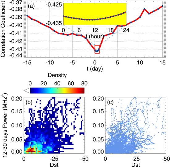
Figure 3. Correlation between the periodic oscillations between 12 and 30 days (mainly 13.5 day and 27 day) in Es layers from the Sodankylä ionosonde and the magnetic activity Dst index during 1993–2018. (a) Cross-correlation coefficient between the 12 and 30 day wavelet power in foEs and the 27 day smoothed daily minimum Dst index as a function of time lag t. (b) and (c) Density scatter plot and scatter plot of the 27 day smoothed daily minimum Dst vs. the 12–30 day wavelet power with the maximum cross-correlation at a time lag of 11 hr. The observations in the density scatter plot were binned in 1.0 (Dst) × 0.005 MHz2 (wavelet power).
Download figure:
Standard image High-resolution imageFigure 4 corresponds to Figure 3 but uses the Ap geomagnetic index instead of Dst: it shows the correlation between the oscillations at periods of 12–30 days in Es layers from the Sodankylä ionosonde and the magnetic activity Ap index during 1993–2018. The cross-correlation function between the 12–30 day wavelet power of foEs and the 27 day smoothed daily Ap index as a function of time lag is shown in Figure 4(a). The maximum cross-correlation is 0.402 at a time lag of 25 hr. The different time lags are consistent with the different responses of Dst and Ap indices to the interplanetary magnetic field (IMF) (Davis et al. 1997; McPherron et al. 2004; Adebesin 2016). The Dst index shows a decrease several hours after the southward turnings of the IMF (Lockwood et al. 2016a), while the Ap index shows a rise around the time of the southward turnings. The time delay between these two geomagnetic activity indices is approximately 14 hr, based on the analyses of the maximum cross-correlations in Figures 3 and 4. The density scatter plot and scatter plot of the 27 day smoothed daily mean Ap versus the 12–30 day wavelet power for the maximum cross-correlation are shown in Figures 4(b) and (c). The observations in the density scatter plot were binned in 0.6 (Ap) × 0.005 MHz2 (wavelet power).
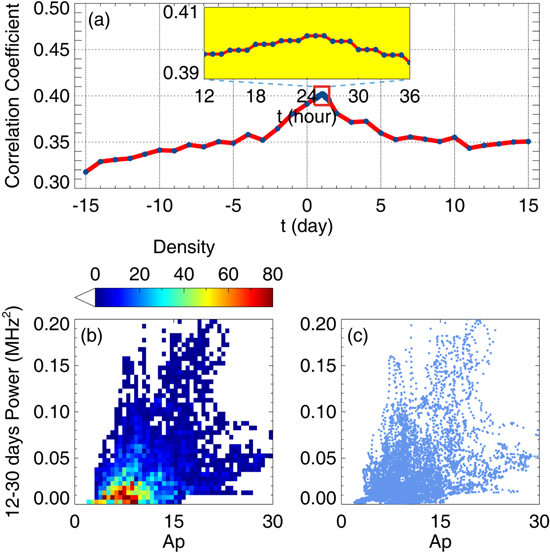
Figure 4. Correlation between the periodic oscillations between 12 and 30 days (mainly 13.5 days and 27 days) in Es layers from the Sodankylä ionosonde and the magnetic activity Ap index during 1993–2018. (a) Cross-correlation coefficient between the 12–30 day wavelet power of foEs and the 27 day smoothed daily mean Ap index as a function of time lag t. (b) and (c) Density scatter plot and scatter plot of the 27 day smoothed daily mean Ap vs. the 12–30 day wavelet power with the maximum cross-correlation at a time lag of 25 hr. The observations in the density scatter plot were binned in 0.6 (Ap) × 0.005 MHz2 (wavelet power).
Download figure:
Standard image High-resolution imageFigure 5 shows the results of the wavelet analysis of foEs at Slough (51.5°N, 0.6°W) during the period 1957–1995. The Dst index is available from 1957, therefore the ionosonde data before 1957 are not investigated. The reconstruction of the time series using the wavelet transform has an RMSE of 0.03 MHz. The annual, semiannual, and quasi-seasonal variations are apparent in the wavelet spectrum of foEs in Figure 5(b). However, the 13.5 day and 27 day periodic oscillations in foEs at Slough are not as significant as those at Sodankylä. In Figure 5(c), the peaks at periods of 13.5 and 27 days are both below the 95% confidence level (dashed line). The correlation between the 12–30 day wavelet power and the daily Dst index is not evident as shown in Figure 5(d).
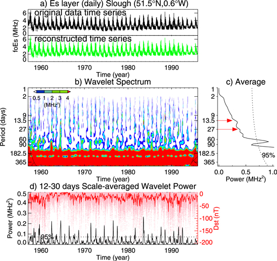
Figure 5. Results of the wavelet analysis of foEs from the Slough ionosonde during 1957–1995. (a) Daily mean original foEs (black), and the reconstructed time series of foEs (green) from the wavelet transform. (b) Wavelet analysis of daily mean foEs using a continuous Morlet transform. (c) Average wavelet power spectrum of foEs. The 95% confidence level is shown as a dashed line. (d) Scale-averaged wavelet power as the weighted sum of the wavelet power spectrum over the periods between 13.5 and 27 days (actually 12–30 days). The variation in the daily 12–30 day scale-averaged wavelet power is shown as a black line. The variation in the 27 day smoothed daily minimum Dst index is shown as a red line, with the hourly Dst index represented by the pink dots.
Download figure:
Standard image High-resolution image3.2. Global Variations in the 27 day Oscillations in Es Layers
The global observations of Es layers can be derived from the amplitude scintillation S4 index from GNSS RO signals. Yu et al. (2020) have derived the global foEs from the COSMIC S4max data during 2006–2014. To investigate the global 27 day oscillations in Es layers and compare with the ground-based observations by ionosondes, the foEs data derived from the COSMIC during 2006–2014 are analyzed. The top panel in Figure 6 shows the foEs along the 60°N–90°N latitude band derived from the COSMIC S4max data. The green line in the bottom panel shows the reconstructed data from the wavelet transform. The reconstruction of time series has an RMSE of 0.01 MHz. Figure 6(b) shows the wavelet spectrum of foEs with enhancements of oscillations at the annual, semiannual, seasonal, 27 day, and 13.5 day periods. The strong fluctuations at periods of 13.5 and 27 days can also be found in the average power spectrum in Figure 6(c), and are at the 95% confidence level (dashed line). A significant 27 day oscillation in Es layers can be found at the high-latitude Sodankylä ionosonde (Figure 2), but not at the midlatitude Slough ionosonde (Figure 5). This indicates that the 13.5 day and 27 day oscillations related to the 27 day solar rotation cycle are dependent on the latitude.
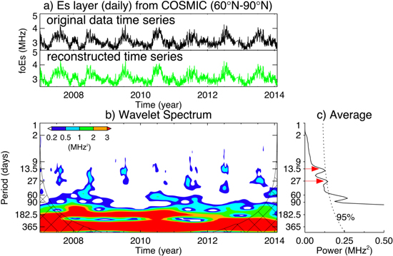
Figure 6. Results of the wavelet analysis of foEs derived from the COSMIC S4max along the 60°N–90°N latitude band during 2006–2014. (a) Daily mean original foEs (black), and the reconstructed time series of foEs (green) from the wavelet transform. (b) Wavelet analysis of daily mean foEs using a continuous Morlet transform. (c) Average wavelet power spectrum of foEs. The 95% confidence level is shown as a dashed line.
Download figure:
Standard image High-resolution imageFigure 7 shows the weighted scaled-averaged wavelet power spectrum of foEs derived from the COSMIC S4max data at different latitude bands during 2006–2014. The 12–30 day (mainly 13.5 day and 27 day) oscillations at high latitudes in the Northern and Southern Hemispheres have a power of 0.02–0.06 MHz2 above the 95% confidence line. The 12–30 day power at high latitudes is stronger than that at midlatitudes and low latitudes. The overall spectrum is consistent with the results from ground-based ionosondes, in which the Es layers present a more significant 27 day oscillation at the high latitude of the Sodankylä ionosonde than at the midlatitude Slough ionosonde. However, there are differences in the temporal behavior shown in Figure 2(b). For the Sodankylä data (Figure 2(b)) the peaks for periods near 27 days occur primarily at sunspot maximum. A similar but smaller solar-cycle dependence is present for the COSMIC data. The high-latitude peaks in the 12–30 day power of foEs are a summer phenomenon: for the Northern Hemisphere they are midway through each calendar year and in the Southern Hemisphere they are near its start, which is consistent with a summer maximum of high-latitude Es layers in previous studies (Kirkwood & Nilsson 2000).

Figure 7. Weighted scale-averaged wavelet power of foEs from the COSMIC S4max between 13.5 and 27 days (actually 12–30 days) in different latitude bands in both hemispheres during 2006–2014. The variations in the daily 12–30 day scale-averaged wavelet power are shown as black lines (high latitudes: 60°–90°), green lines (midlatitudes: 30°–60°), and blue lines (low latitudes: 0°–30°). The 95% confidence level is shown as a dashed line. The variation in the 27 day smoothed daily minimum Dst index is shown as a red line, with the hourly Dst index represented by the pink dots.
Download figure:
Standard image High-resolution imageFigure 8 shows the global map of the scale-averaged wavelet power of foEs at periods of 12–30 days from COSMIC in a 10° × 10° grid during the period 2006–2014. The geomagnetic latitude contours of 60°, 70°, and 80° are represented by red (blue) lines in the Northern (Southern) Hemisphere. The geomagnetic equator is also plotted as a yellow line. The 12–30 day scale-averaged wavelet power of foEs is strong at high latitudes in both hemispheres, indicating that the 13.5 day and 27 day oscillations in Es layers dominate the high-latitude regions. The auroral-type Es layers were found to occur at high latitudes, and are associated with magnetic and auroral activities (Hunsucker & Owren 1962). At high latitudes, the wind shear effect is not as efficient as at midlatitudes (Gubenko et al. 2018; Yu et al. 2019a). Therefore, the auroral Es layers are thought to be caused by magnetic-field-aligned plasma irregularities (Kirkwood & Nilsson 2000). The two-stream and gradient-drift instabilities occur in the auroral region accompanied by strong electric fields (Gubenko et al. 2018). The formation of midlatitude Es layers is mainly controlled by wind shear, and it is modulated less by the 27 day solar rotation. The weak 12–30 day power is visible at midlatitudes between 15° and 45°. In addition, due to the effect of Lorentz forcing on the ion convergence of Es plasma, the weak Es layers form troughs along the 70°N–80°N and 60°S–70°S geomagnetic latitude bands (Yu et al. 2019a), and thus present weak 12–30 day oscillations. Another interesting feature is the relatively strong 12–30 day wavelet power of Es layers near the magnetic equator. The formation of the equatorial Es layers is attributed to the magnetic-field-aligned irregularities associated with the equatorial electrojet. The formations of auroral and equatorial Es layers are both associated with an intense current flow, which is found to increase with intense magnetic activities (Whitehead 1970). The auroral and equatorial Es layers with 13.5 day and 27 day periodic oscillations are both modulated by the solar rotation cycles through magnetic activity. In addition, 16 ground-based ionosonde stations, which have at least five years of continuous manually-scaled data at the same period as COSMIC RO data during 2006–2014, are further used to study the 27 day oscillations in Es layers on a global scale. The circles represent the locations of 16 ionosondes used in the wavelet spectrum analysis, with the size of these symbols denoting the 12–30 day wavelet power. It should be noted that the signals of 13.5 day and 27 day periodicities are more clearly identified from the ionosonde observations than the COSMIC satellites. The 12–30 day power of Es layers from ionosondes is generally larger than that from satellites. The details of foEs data from 16 ionosonde stations and the 12–30 day power are listed in order of decreasing north latitude in Table 1.

Figure 8. Global distribution of the scale-averaged wavelet power of foEs at periods of 12–30 days from COSMIC in a 10° × 10° grid during 2006–2014. The locations of 16 ionosonde stations are shown as circles with the 12–30 day wavelet power of foEs from each ionosonde represented by the size of symbols. The details of ionosonde stations are listed in Table 1. The geomagnetic equator and the geomagnetic latitudes of 60°, 70°, and 80° in the Northern and Southern Hemispheres are plotted.
Download figure:
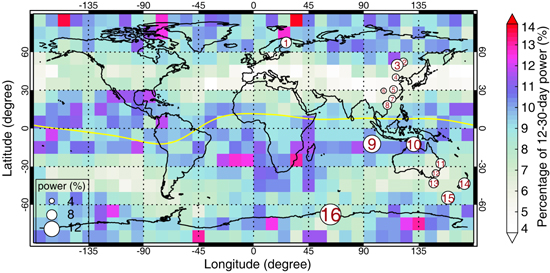
Standard image High-resolution imageFigure 9 shows the percentage of the scale-averaged wavelet power of foEs at periods of 12–30 days from COSMIC in a 10° × 10° grid during the period 2006–2014. The global map of wavelet power shows a significant enhancement within low-latitude and high-latitude bands. The 12–30 day oscillations account for 10%–14% of all variations in foEs at low latitude and high latitude. The 12–30 day power of foEs is 4%–10% at midlatitudes. This reveals that the 13.5 day and 27 day periodic oscillations in the Es layers are evident at low latitudes and high latitudes, but are not significant at midlatitudes. The wavelet spectral results of 16 ground-based ionosonde stations present a consistent result, with the percentage of the 12–30 day power represented by the size of the circles on the map.
Figure 9. Global distribution of the percentage of the scale-averaged wavelet power of foEs at periods of 12–30 days from COSMIC in a 10° × 10° grid during 2006–2014. The locations of 16 ionosonde stations are shown as circles with the 12–30 day wavelet power of foEs from each ionosonde represented by the size of symbols.
Download figure:
Standard image High-resolution image
4. Discussion and Conclusions
We have reported a signature of the 27 day periodic oscillation (and its harmonic) in the Es layers associated with the 27 day solar rotation period. The pronounced periodicities of 27 and 13.5 days are dependent on latitude. The equatorial and auroral Es layers present significant 13.5 day and 27 day periodic oscillations. The power of the 12–30 day (mainly 13.5 day and 27 day) wavelet spectra accounts for 10%–14% of all variations in foEs at low latitudes between 0° and 15° and high latitudes between 45° and 90°. The weak 12–30 day oscillations are visible at midlatitudes between 15° and 45°, and account for 4%–10% of all variations in foEs. The 27 day and 13.5 day oscillations in high-latitude Es layers correlate well with the geomagnetic Dst and Ap activity indices. The spectral analyses suggest that the 27 day periodic oscillations of the terrestrial metallic ions within Es layers are associated with recurrent geomagnetic activities, which are related to high-speed solar winds generated from persistent coronal holes on successive 27 day solar rotations. The 13.5 day and 27 day oscillations in the Es layers become more evident at solar maximum (2000–2003 and 2011–2014) than at solar minimum.
The diurnal and semidiurnal atmospheric tides are well known to dominate the short-term variations in Es layers (MacDougall 1974; Cai et al. 2017; Yu et al. 2020). The diurnal tidal modulation is significant at low latitudes between 0° and 30° and high latitudes between 75° and 90°. The semidiurnal tidal modulation is significant at midlatitudes between 30° and 75° (Yu et al. 2020). Gravity waves and planetary waves (PWs) also have an effect on Es layers (Haldoupis et al. 2004; Gu et al. 2014; Yuan et al. 2014). The 7 day PW periodicity was found in the time series of foEs from a longitudinal chain of ionosondes in 1993 August–September, and presents a link between Es layers and PWs (Haldoupis & Pancheva 2002). Our study reveals that the 27 day solar rotation modulates the abundance of metallic ions within Es layers and contributes to the 9 day, 13.5 day, and 27 day periodicities in the short-term variability of Es layers.
Wu et al. (2019) reported a 27 day response of neutral metal layers to the solar rotation in the mesosphere and lower thermosphere regions. The mean column density of modeled Na, K, and Fe atoms decreases approximately 3% with rising temperature in response to the 7% increase in solar spectral irradiance. The changes of neutral metal layers are explained by the role of ion–molecule chemistry due to the temperature anomalies. The 27 day response of metal layers is significantly stronger at solar maximum than at solar minimum. As shown in Figure 2, the metallic ions within Es layers represented by foEs from a high-latitude ionosonde at Sodankylä, Finland, contain 13.5 day and 27 day oscillations related to the 27 day solar rotation. The 13.5 day and 27 day oscillations in metallic ions are much stronger at solar maximum than at solar minimum. The 27 day responses of metallic ions are likely associated with those of metal atoms, because the metal composition in the upper atmosphere is dependent on the interaction of chemical reactions, photochemical reactions, and electrodynamics (Plane et al. 2015). The atomic O mixing ratio increases in response to enhanced EUV radiation (Wu et al. 2019). The increased O reduces molecular ions back to atomic metal ions (e.g., FeO+ + O → Fe+ + O2), and thus prevents dissociative recombination to neutral metal atoms. Besides, dielectronic recombination of the metal ions (Fe+ + e− → Fe + h ν), and the recombination reactions from metal ions to form molecular ion clusters (Fe+ + N2 + (M) → Fe+ · N2) that then recombine with electrons, both have negative temperature dependences. The recombination reactions get slower with rising temperature in the mesosphere and lower thermosphere (MLT) region. The metal atoms decrease and metal ions increase in response to increasing solar irradiance. Therefore, the ion–molecule chemistry caused by temperature anomalies, associated with the 27 day periodic solar rotation, would be expected to influence the abundance of metallic ions in the ionosphere. The 9 day periodic variation was found in the meridional component of diurnal tides (Yi et al. 2021), and could potentially enhance the wind shear necessary to form an Es layer.
In Figure 9, the low-latitude Es layers occurring over oceans tend to present stronger 13.5 day and 27 day oscillations than those over the continents. It has been shown that negative cloud-to-ground strokes with large impulse charge moments and high peak currents are predominantly produced in oceanic thunderstorms (Sato & Fukunishi 2003). The associated halo (spatially diffuse glow within the nighttime lower ionosphere at 80 km altitude), occurs more frequently above oceanic thunderstorms (Lu et al. 2018). The electric field and gravity waves generated by intense thunderstorms can affect the lower ionosphere (Davis & Johnson 2005; Davis & Lo 2008; Yu et al. 2015). Rahmani et al. (2020) showed clear influences of thunderstorms on the lower ionosphere by using GNSS data. There is evidence that lightning rate is modulated by high-speed solar wind streams at Earth (Scott et al. 2014a). The heliospheric magnetic field (HMF) in near-Earth space typically reverses within a CIR and it can influence the lightning rate (Owens et al. 2014). The CIR effect on lightning is proposed to result from compression of the HMF and its interaction with the terrestrial system via the global electric circuit (Lam et al. 2013). The strong 27 day oscillations in metallic ions within Es layers at altitudes between 90 and 130 km indicate a modulation associated with CIRs, which affects the local ionospheric potential and perturbs the atmospheric electric circuit (Wilson 1921), and hence couples into weather-forming regions (Owens et al. 2015).
The persistent CIR pattern was particularly pronounced between 2007 and 2008, when the 27 day periodic variation in atmospheric electricity becomes apparent (Harrison et al. 2013). During the 2007–2008 solar minimum, the 27 day cyclic atmospheric changes were related to solar-induced variations in energetic particles, but not related to variations in solar UV radiation (Harrison & Lockwood 2020). In Figure 2(b), a similar individual signal of 27 day periodic oscillations in Es layers during the 2007–2008 solar minimum was also found in the wavelet spectrum of foEs. It shows that the strong 27 day cyclic change of metallic ions within Es layers occurs not only at solar maximum, but also at solar minimum when there is a strong solar rotation effect. Because plasma irregularities in Es layers can significantly affect radio communications and navigation systems (Yue et al. 2016; Yu et al. 2021), any predictable influence on the reliability of these systems, even during the solar minimum, is very important to quantify given the growth in demand for high-accuracy and reliable GNSS applications.
We acknowledge the UK Solar System Data Centre (UKSSDC) at the Rutherford Appleton Laboratory, the Chinese Meridian Project, the Solar–Terrestrial Environment Research Network (STERN), and the Geophysics Center, National Earth System Science Data Center at BNOSE, IGGCAS for providing the ionospheric data. We acknowledge the Constellation Observing System for Meteorology, Ionosphere, and Climate (COSMIC) Data Analysis and Archive Center (CDAAC) for providing COSMIC radio occultation data. The authors would like to thank the National Science & Technology Infrastructure of China. This work has been supported by the B-type Strategic Priority Program of CAS (grant No. XDB41000000), the National Natural Science Foundation of China (grant Nos. 41774158, 41974174, 41831071), the Project of Stable Support for Youth Team in Basic Research Field, CAS (grant No. YSBR-018), the CNSA pre-research Project on Civil Aerospace Technologies (grant No. D020105), Anhui Provincial Natural Science Foundation (grant No. 1908085QD155), and the Fundamental Research Fund for the Central Universities. Bingkun Yu was supported by the Royal Society for the Newton International Fellowship (grant No. NIF\R1\180815).
The ionosonde data are available from the UKSSDC at the Rutherford Appleton Laboratory (https://www.ukssdc.ac.uk), the Data Centre for Meridian Space Weather Monitoring Project (https://data.meridianproject.ac.cn), and the Geophysics Center, National Earth System Science Data Center at BNOSE, IGGCAS (http://wdc.geophys.ac.cn). The COSMIC satellite radio occultation data are available from the CDAAC website (https://data.cosmic.ucar.edu/gnss-ro/). The global critical frequency foEs data derived from the COSMIC S4max in the period 2006–2014 are available in the Dryad data repository (doi.org/10.5061/dryad.xsj3tx9bx). The wavelet software was provided by C. Torrence and G. Compo, and is available at URL: http://atoc.colorado.edu/research/wavelets/.