


Abstract
X-ray observations are limited by the background, due to the intrinsic faintness or diffuse nature of the sources. The future Athena X-ray observatory has among its goals the characterization of these sources. We aim at characterizing the particle-induced background of the Athena microcalorimeter, in both its low- (soft protons) and high-energy (galactic cosmic rays—GCR) induced components, to assess the instrument capability to characterize background-dominated sources such as the outskirts of clusters of galaxies. We compare two radiation environments, namely the L1 and L2 Lagrangian points, and derive indications against the latter. We estimate the particle-induced background level on the X-IFU microcalorimeter with Monte Carlo simulations, before and after all of the solutions adopted to reduce its level. Concerning the GCR-induced component, the background level is compliant with the mission requirement. Regarding the soft-proton component, the analysis does not predict dramatically different backgrounds in the L1 and L2 orbits. However, the lack of data concerning the L2 environment labels it as very weakly characterizable, and thus we advise against choosing it as the orbit for X-ray missions. We then use these background levels to simulate the observation of a typical galaxy cluster from its center out to 1.2 R200 to probe the characterization capabilities of the instrument out to the outskirts. We find that without any background reduction, it is not possible to characterize the properties of the cluster in the outer regions. We also find no improvement in the observations when carried out during the solar maximum with respect to solar minimum conditions.
Export citation and abstract BibTeX RIS
1. Introduction
Athena (Nandra et al. 2013) is the second large-class X-ray mission of the European Space Agency Cosmic Vision program, with a launch foreseen in early 2030 toward an L2 halo orbit and dedicated to the study of the hot and energetic universe. The mission couples a high-performance X-ray telescope (1.4 m2 at 1 keV and an angular resolution of 5'') with two complementary focal-plane instruments, the Wide Field Imager (WFI) optimized for surveys (Meidinger et al. 2018) and the X-ray Integral Field Unit (X-IFU), providing integral-field spatially resolved high-energy-resolution spectroscopy (2.5 eV at 6 keV) over a 5' field of view (FoV) in the 0.2–12 keV energy band, thanks to an array of ∼3840 transition-edge sensor (TES) microcalorimeters operated at 50 mK with a 249 μm pitch for a 2.3 cm2 sensitive area (Barret et al. 2018).
X-ray observations are usually severely limited by the background, due to the intrinsic faintness of the astrophysical sources involved or to their diffuse nature, and this is especially true for Athena, which has among its goals the characterization of faint/distant/diffuse sources unobservable with any other present or planned instrument (Nandra et al. 2013). For this reason, substantial effort has been dedicated to the assessment of the expected background level.
In this paper, we address the particle-induced background of the X-IFU instrument and assess the capability of the mission to characterize background-dominated sources, discussing the specific case of the outskirts of clusters of galaxies.
This paper is structured as follows: in Section 2, we introduce general issues with the background of X-ray instruments; in Section 3, we focus on the methodology used to estimate the particle background induced on the X-IFU. In Section 4, we report the results of the high-energy induced component of the particle background, while in Section 5, we do the same for the low-energy induced component. In Section 6, we use the background levels calculated in the previous sections to estimate the X-IFU observation capabilities of a galaxy cluster outskirt out to 1.2R200, and in the final section, we report our conclusions.
2. The Background of the X-Ray Instruments
X-ray instruments are subject to different kinds of backgrounds of different nature and features.
The first component, dominant at E < 2 − 3 keV, is induced by the cosmic X-ray background (CXB), a diffuse X-ray emission observed in every direction. At low energies (<1 keV), it is composed of several contributions, each with its own spatial and temporal variations, while at higher energies, it is generated by the unresolved emission from active galactic nuclei (AGNs). This component is induced by photons produced by X-ray sources in the sky; it reaches the detector from the optics and can be damped only by resolving the AGN-induced component into the single sources that create it.
The second component is generated by charged particles and can be further divided into two separate contributions:
- 1.Low-energy particles (soft protons—SP), mostly protons below 200 keV, that follow a path similar to the CXB, being concentrated by the mirrors onto the focal plane and releasing all of their remaining energy in the detectors.
- 2.High-energy particles (galactic cosmic rays—GCR) that possess enough energy to travel through the spacecraft and reach the detector from any direction, typically releasing inside it a small fraction of their energy. These particles also create showers of secondary particles (mostly electrons) along the way, which can also induce additional background.
In this paper, we deal with both the contributions of the second component, while for the first we assume the modeling reported in Lotti et al. (2014).
3. The Particle Background Estimation
There are no data available for X-ray microcalorimeters in L2 (or L1) at the moment of writing, thus it is impossible to estimate the expected background level relying on existing data. The problem is also too complex to face using an analytical approach, and consequently, the background estimates are performed using Monte Carlo simulations with the Geant4 software (Agostinelli et al. 2003; Allison et al. 2006, 2016).
Geant4 is a toolkit that provides access to several different models to reproduce physical processes the user is interested in. Also, it is possible to set the simulation detail level to suit the user's needs, balancing the accuracy of the results with the simulation speed.
Thanks to this tool, it is possible to create a virtual model of the instrument and its surroundings (the so-called mass model) and of the particle environment it will be placed into, and analyze how they interact with each other and ultimately, given the proper settings, to predict the expected instrument performances, among which is the background level. Furthermore, it is possible to test the effect of changes to the instrument mass model (sensitivity analysis) and identify the configuration that optimizes the detector performances.
We have exploited this Monte Carlo tool to estimate the impact of both the GCR-induced component and the SP-induced one.
3.1. Input Spectra
The Athena mission is foreseen to fly in the L2 Lagrangian point. However, the possibility of directing the spacecraft in the L1 point is under discussion. We report here the results of the analysis of the environment of the two orbits.
Regarding the GCR component, it changes through the solar system with the distance from the Sun, and L1 and L2 are close enough to not expect any significant difference between the two orbits (ΔR/ < R > ∼ 2%, with R the distance from the Sun). The reference spectra are listed in the following and shown in Figure 1.

Figure 1. Left: input spectra for GCR protons, GCR alpha particles, and electrons (both GCR and Jovian contribution). Right: L1 and L2 input fluxes for solar wind (the most probable environment) and for the worst case foreseen in both environments. See text for details.
Download figure:
Standard image High-resolution imageThe reference model for GCR protons has been described in Usoskin et al. (2005); here we report the formula for the differential intensity J of cosmic-ray nucleons at 1 au in particles cm−2 s−1 sr−1 GeV−1:

where

is the local interstellar spectrum (LIS) of cosmic-ray nuclei. E is the kinetic energy of the particle in GeV, Er = 0.938 GeV is the proton rest mass, and ϕ is the modulation potential in GV, also known as the "force field parameter" and the "modulation strength," and represents the mean energy loss of the GCR particle inside the heliosphere. We used this model to fit satellite data for 2009 from SOHO (Kühl et al. 2016), Pamela (Adriani et al. 2013), and Voyager, obtaining ϕ = 0.3793 ± 0.0014 GV for the GCR maximum (solar minimum). We chose 2009 as a reference year because it corresponds to a solar minimum in a solar cycle with the same negative polarity as the one in which Athena will operate (Adriani et al. 2013), and we use it as a proxy for the year 2031 in which maximum GCR flux is expected for cycle 26. This spectrum was checked against the heliospheric modulation model (Boschini et al. 2019) results for 2009, and resulted in an agreement for E > 1 GeV and conservative at energies below. Regarding the GCR minimum (solar maximum) that will be possibly experienced by Athena during its lifetime, we kept using solar cycle 24 as a proxy for solar cycle 26 in which Athena will fly, and used the year 2014 as the solar maximum to be experienced by Athena during its lifetime, fitting SOHO data to obtain an expected ϕ = 0.803 ± 0.01 GV value as the GCR minimum in that timeframe.
The alpha particles spectrum has been evaluated from the Kuznetzov empirical model (Kuznetsov et al. 2017) for quiet-Sun conditions:

where E is the kinetic energy per nucleus in MeV and FHe is in particles cm−2 s−1 sr−1 MeV−1. The adopted spectra correspond to quiet-Sun conditions, where the Sun's magnetic shielding effectiveness is at its lowest, thus providing the maximum alpha particles flux. The adopted alpha particles spectrum was checked against the heliospheric modulation model (Boschini et al. 2018, 2019, 2020) results for 2009 and resulted in perfect agreement.
The high-energy end (>3 GeV) of the GCR electrons spectrum was fitted as a power law from Pamela data for 2009 (Adriani et al. 2015):

where E is the kinetic energy in GeV and  is in particles m−2 s−1 sr−1 GeV−1. At lower energies, we decided to take into account the role of interplanetary (Jovian) electrons. We fitted the spectra reported in Grimani et al. (2009) for a negative polarity period, for the maximum Jovian component:

and for the minimum Jovian component:

These spectra were checked against the heliospheric modulation model (Boschini et al. 2018, 2019) results for 2009, and our modeling choice resulted in agreement.
According to the latest formulation, the Athena background requirement should be satisfied by the assumption of an external reference flux equal to 80% of the GCR maximum flux, which is what we refer to in all of the following.
Once the largest flux conditions were established, we investigated the expected GCR protons flux variability from cycle to cycle. There is a correlation between the neutron monitor count rates on Earth (Usoskin 2001), which are part of long-term cosmic-ray measurements taken from Earth's surface, and the integrated GCR protons flux, so we analyzed the neutron monitor count rate collected from 1964 up to 2017 to establish the variability from cycle to cycle. During this time span, five different solar cycles occurred: three of them characterized by a heliosphere with a negative polarity (solar minima in 1965, 1987, and 2009), such as the one expected in the Athena lifetime (Adriani et al. 2013). Analyzing the neutron monitor counts over a 2 yr average around the solar minima, the GCR flux indetermination is ∼26%. This estimate is, however, based on a very small sample (three solar minima with negative polarity since 1964). If we compute the population variance at the 95% confidence level, the resulting indetermination can be up to six times larger than the sample variance.
Regarding the SP component, which belongs in the hundreds of keV regime, important effort has been spent in characterizing the two possibilities under discussion for the Athena orbit, namely the L1 and L2 Lagrangian points of the Earth–Sun system. The spectral shapes for the SP detected by several satellites present in L1 and L2 (Lotti et al. 2018; Laurenza et al. 2019) are reported in Table 1. The integrated fluxes in 40–80 keV are reported in Table 2.
Table 1. Proton Flux Fit Functions for Different Thresholds, Valid for the 50–5000 keV Energy Range
| Cumulative Probability | Fit Function |
|---|---|
| Solar Wind 50% (L1) |

|
| Solar Wind 90% (L1) |

|
| Solar Wind Worst Case (L1) |

|
| Quiet Magnetosheath (L2) | 8.6 × 10⁵ · E−2.94 |
| Magnetosheath Worst Case (L2) | 7 × 10⁶ · E−3.11 |
Note. E is the kinetic energy in keV, flux is in particles cm−2 s−1 sr−1 keV−1. SW stands for solar wind, while MS stands for magnetosheath.
Download table as: ASCIITypeset image
Table 2. Summary Table of the Relevant Numbers
| Integrated Input Flux (40–80 keV) | Flux at FPA Level | Fraction to Block | E to Block | |
|---|---|---|---|---|
| (p cm−2 s−1 sr−1) | (p cm−2 s−1) | (keV) | ||
| Solar Wind 50% (L1) | 18.5 | 8.3 × 10⁻⁴ | ⋯ | ⋯ |
| Solar Wind 90% (L1) | 183.8 | 8.46 × 10⁻³ | 52.72% | 57 |
| Solar Wind Worst Case (L1) | 751.1 | 3.47 × 10⁻² | 88.47% | 65 |
| Quiet Magnetosheath (L2) | 255.7 | 10−2 | 60.00% | 58 |
| Magnetosheath Worst Case (L2) | 1054.6 | 4 × 10⁻² | 90.00% | 66 |
Note. The fractions and energies to block for the 50% solar wind case are not reported because the corresponding fluxes at the FPA level already satisfy the requirement.
Download table as: ASCIITypeset image
Observations of the ARTEMIS probes (Angelopoulos 2011) simultaneously obtained in both the solar wind and distant magnetotail have shown that the L2 SP fluxes are similar to the ones measured at L1 but with the superimposition of an important component fed by the particles accelerated inside the magnetosphere as soon as there is some geomagnetic activity, which is very often.
We emphasize that all available data related to the L2 environment comprises only a few months of data close to the L2 point in a 2 yr period, i.e., only covering a small fraction of a single solar cycle. Moreover, we point out that these 2 yr occurred during the solar cycle decreasing phase. Due to this very limited coverage, the knowledge of the SP fluxes in L2 is much more limited with respect to the one inferred from the corresponding L1 data set, which involves tens of years of data along two solar cycles. Consequently, despite having performed the work for both cases, it is not possible to produce a reliable forecast of the L2 SP fluxes, and the L1 estimates should be considered the only reliable ones.
3.2. X-IFU Mass Model
In 2017, we received updated drawings of both the cryostat from CNES (Centre National D'Etudes Spatiales) and the FPA (focal-plane assembly) from SRON (Netherlands Institute for Space Research), respectively, from which we derived an updated version of the Geant4 mass model of the X-IFU. The engineering CAD models received were far too detailed and complex for insertion into the Monte Carlo code, so substantial simplification work has been carried out, stripping the model of unnecessary details while preserving the masses and shapes as much as possible (see Figure 2). The level of detail increases closer to the detectors, which are modeled in the greatest detail (all ∼3840 pixels of the main detector are present and modeled according to the latest layout available at that time).

Figure 2. CAD of the simplified mass models used in the Geant4 simulations: cryostat (left) and FPA (right).
Download figure:
Standard image High-resolution imageIn the basic FPA configuration, the detector is directly exposed to the niobium cryogenic shielding, but in the latest baseline, a passive shielding was introduced in order to reduce the flux of secondary particles. We investigated the background expected on the detector in both configurations.
4. The Background Foreseen for the X-IFU: The High-energy Component
As the GCR protons are the dominant component of the external particle flux when compared to electrons and alpha particles (and of the residual background, as we will see in the following), we perform most of the analysis on this component, and once the optimal configuration for the background has been established, we also simulate the other particle species.
Without any kind of reduction technique, the X-IFU would experience a GCR-proton-induced background level of (148 ± 0.08) × 10−3 cts cm−2 s−1 keV−1 in the 2–10 keV energy band, 30 times above the 5 × 10⁻³ cts cm−2 s−1 keV−1 requirement (see Figure 3). For this reason, a cryogenic anticoincidence detector (CryoAC) was introduced into the baseline configuration. This reduced the unrejected background level down to (4.8 ± 0.16) × 10−3 cts cm−2 s−1 keV−1, efficiently discriminating against high-energy particles that can cross the main detector and reach the CryoAC. Assuming a 20% margin due to the systematic uncertainty on the Geant4 reproducibility of in-flight background data, as found by the accuracy of the simulations (Ozaki & Fioretti 2018), the background level is 20% above the requirement. This evaluation was performed taking into account only GCR protons (which produce ∼70% of the residual particle background), while later on we report the expected full contribution.

Figure 3. Background levels in different FPA configurations.
Download figure:
Standard image High-resolution imageThe analysis of the residual background composition and origin revealed that this background is induced mainly by secondary electrons coming from the niobium shield surrounding the detector that impact the X-IFU from above and backscatter on its surface, releasing a small fraction of their energy (see Figure 4). To reduce this component, we tested the secondary electron yield from different materials and designed a passive low-Z shield to interpose between the detector and the niobium. This introduction of the Kapton shield allowed the residual background level induced by GCR protons to be further damped down to (3.6 ± 0.16) × 10−3 cts cm−2 s−1 keV−1.
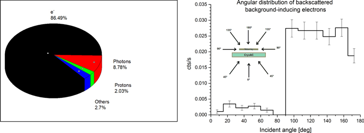
Figure 4. The residual background composition (left) and the angular distribution of the incident directions of the backscattered electron component (right). The plots were produced using GCR protons as input.
Download figure:
Standard image High-resolution imageAfter the Kapton insertion, the background showed a significant contribution (∼10%) from 16 and 18 keV niobium fluorescence lines that induce escape peaks on the detector. To prevent these fluorescence photons from reaching the detector, several improvements to the passive shielding were tested (Lotti et al. 2017), and finally, the best option for the passive shield was found to be 10 μm of bismuth followed by 250 μm of Kapton, which allowed the level of (2.96 ± 0.16) × 10−3 cts cm−2 s−1 keV−1 to be reached
These background levels were obtained by applying different screening strategies:
- 1.Time coincidence with the CryoAC: photons do not produce a coincidence signal in the X-IFU-CryoAC system, so we can assume that every event that is detected simultaneously (Δt < 10 μs) in both the CryoAC and the main detector can be rejected as a particle-induced one. A CryoAC low-energy threshold of 20 keV is considered.
- 2.Pattern recognition: due to the detector features (no charge cloud diffusion among different pixels as in CCD-like detectors, pixels physically separated), source photons will not produce pixel patterns complicated to reconstruct. Instead, we can assume that all events that turn on more than one pixel can be rejected as induced by particles with skew trajectories intersecting more than one pixel, or as simultaneous impacts by multiple particles associated with the same primary.
- 3.Energy deposition: given the steep decrease of the optical effective area outside the detector energy band, we can assume that all events that deposit energy outside the instrument sensitivity band are due to charged particles and, therefore, reject them.
We performed an investigation of the geometrical origin of the unrejected background. Before the shield introduction, a major fraction of the background is induced by the 50 mK niobium shield, this being the last surface directly seen by the detector. After the Kapton/Bi insertion, the contribution from this surface is now mostly blocked by the passive shield, going from 80% contribution to 12%. Even though the passive shield has now become the relative main background source, due to a lower electron production yield, the absolute background level has been reduced. The corresponding spectra and background level have been reported in Figure 3.
Regarding the residual background particle composition, backscattered electrons produced in the surfaces directly seen by the detector have repeatedly proven to be the main component of the residual background after the insertion of the CryoAC (Lotti et al. 2017, 2018), because ∼85% of the residual background is induced by secondary electrons and ∼80% of these electrons are backscattered. Moreover, we investigated the angular distribution of the backscattered electrons. These particles impact the detector surface and bounce back, releasing a small fraction of their energy (dependent on the impact angle). As can be seen from Figure 4 (right), almost no electrons backscatter on the lower side of the detector, as the CryoAC efficiently blocks/vetoes those particles, while the major contribution comes from above, as expected. The distribution itself is quite flat, indicating no preferential direction from where these electrons come from, aside from a dip around the direction normal to the detector surface. An analysis of the FPA geometry reveals that this corresponds roughly to the FoV opening angle, the direction where there is almost no mass to produce the secondary electrons.
Using the updated mass model in the baseline configuration (Kapton/Bi passive shield), we investigated the impact on the background of the other environmental particle populations expected to be present in L2, namely GCR alphas and electrons. Our analysis reported a total background level of (4.34 ± 0.21) × 10−3 cts cm−2 s−1 keV−1 in the 2–10 keV energy band, compliant with the scientific requirement, as can be seen in Figure 5. Even if we take into account the 20% margin, the foreseen background level is still compliant with the requirement at the 1σ level.

Figure 5. The unrejected particle background of the X-IFU instrument (black line) and all its contributions: GCR protons (red line), alpha particles (magenta line), and electrons (blue line).
Download figure:
Standard image High-resolution image4.1. Expected Variations during the Mission Lifetime
We investigated the expected variations in the unrejected background level during the mission lifetime, as the GCR flux intensity is anticorrelated with solar phases. We simulated both the maximum and minimum GCR spectra measured in solar cycle 24 after 2009 (years 2009 and 2014 respectively; Figure 6, left) on the X-IFU mass model and obtained the results shown in Figure 6 (right).

Figure 6. Expected input spectra for the GCR maximum and minimum during the Athena mission lifetime (left). Unrejected background spectra resulting from the input spectra are on the left (right). Integrated fluxes refer to the 100 MeV–100 GeV energy band. The residual background scales linearly with the integrated input fluxes.
Download figure:
Standard image High-resolution imageThe spectral shape of the unrejected background in the 2–10 keV energy band was not affected sensibly by the change in spectral shape, and the integrated value scaled linearly with the integrated fluxes in the 100 MeV–100 GeV energy band.
Regarding the Jovian component of the GCR electrons spectrum, which is expected to vary according to the relative position of Earth and Jupiter during the mission, we expect no significant variation in the induced background spectrum (Figure 5).
4.2. Future Updates
The reported results are based on an X-IFU mass model developed from CAD delivered by CNES and SRON in 2017. The FPA design is constantly under improvement, and since then it has been slightly modified. To establish the impact of such modifications, a sensitivity analysis has been performed on some items (see Appendix B and Figures 13 and 14). The main differences present with respect to the current design are as follows:
- 1.It is necessary to change bismuth to gold as a second layer of the passive liner (Kapton based).
- 2.The radiation filter modeling needs to be updated to the latest design. In particular, the 50 mK filter will be placed at the bottom of the Nb shield and not at the top.
- 3.The lower edge of the passive liner must be at a minimum distance higher than 2 mm.
- 4.The CryoAC rim needs to be updated, changing the upper 500 μm from copper to silicon, according to the latest development.
- 5.The detector pixel layout needs to be updated to the latest design.
Furthermore, the simulation settings and post-processing can be improved with:
- 1.new settings of the CryoAC detector to improve simulation performances, and
- 2.post-processing of the output will be redefined to mimic the actual detector pipeline.
Most of the bullets have a direct impact on the FPA design. Thanks to the sensitivity analysis performed, we have solutions to mitigate the impact of these differences on the residual particle background: it is again the use of a well-shaped Kapton/gold liner both around the 50 mK filter metallic frame and on the inner cylindrical surface of the Nb shield. A new set of Geant4 simulations will be performed once the FPA design becomes more mature.
5. The Background Foreseen for the X-IFU: The Low-energy Component
SP in the ∼100 keV energy range are funneled by the X-ray optics toward the focal plane and have proven to be a major hindrance to the sensitivity of X-ray missions, decreasing by about 40%–50% the usability of the data for background-sensitive observations and contaminating the remaining data with a poorly reproducible background component (see Lotti et al. 2018 and references therein).
The challenging scientific goals of Athena, such as the observation of faint/diffuse/distant sources, impose that SP-induced background can contribute up to a maximum of 10% of the high-energy particle background requirement (which corresponds to a flux of 5 × 10⁻⁴ cts cm−2 s−1 keV−1 in the 2–10 keV energy band). The solution is to introduce a high magnetic field between the mirrors and the detectors to deflect these particles away from the instruments' FoV.
5.1. Mirror Funneling and Filter Stack Transmission Efficiency
The optics funneling efficiency has been calculated by ray-tracing simulations and cross-checked with Geant4 simulations, while the filter transmission efficiency has been characterized by the X-IFU team using a series of mono-energetic simulations (see Figure 7, left). This information has been used to construct a proton response matrix, analogous to the one used for photons. Details on the adopted approach are reported in Lotti et al. (2018).

Figure 7. Filter transmission efficiency for soft protons for X-IFU, as calculated with Geant4 simulations (left). The expected spectra of the initial energies of the protons that induce a background in the 2–10 keV energy range in L1, for the worst case in L1 and the worst L2 case of the active magnetosheath (right), assuming no magnetic diverter.
Download figure:
Standard image High-resolution image5.2. The Expected Fluxes at the Focal Plane Level
The response matrices and external fluxes have been used to calculate the expected fluxes and spectra of the initial energies of the protons that induce a background in the 2–10 keV band at the focal plane level, as can be seen in Figure 7 for L1 and the L2 worst cases (Lotti et al. 2018). The initial energy spectral distribution of the particle inducing background on the X-IFU is shaped mostly by the transmission of the filters rather than the differences in the slopes of the input spectra.

Figure 8. The GCR-induced particle background level considered in the analysis (left) and the total background used in the simulations, including the CXB contribution (right) that starts being dominant below 2 keV. The black line is the "No CryoAC" background level, the red line is the "Best Estimate," and the green line is the "GCR min."
Download figure:
Standard image High-resolution imageThe integrated background levels for all cases considered are reported in Table 2. Comparing the integrated background levels to the requirement (5 × 10⁻⁴ cts cm−2 s−1keV−1 or, equivalently, 4 × 10⁻³ cts cm−2 s−1), we can calculate the required fraction of flux to be blocked by the foreseen magnetic diverter and from the cumulative curve of the spectral distributions, the required energy threshold of such diverter, reported in Table 2.
The analysis did not show dramatically different flux levels when comparing the two orbits, even though the L1 orbit seems to be favored in every condition. Consequently, there is not a huge impact of the orbit on the threshold energy to be blocked by the magnetic diverter.
We remark once again that the coverage of the L1 data is extremely higher than the one relative to the L2 data, as the latter were obtained during just 2 yr close to the L2 point, i.e., only covering a particular fraction of a single solar cycle. Conversely, we have tens of years of data accumulated by several satellites to characterize the L1 point.
6. Impact of the Background on the Observation of Galaxy Clusters with X-IFU
One of the primary goals of the Athena X-IFU is to probe the diffuse plasma that fills the potential wells of galaxy clusters (the intracluster medium, ICM; Ettori et al. 2013; Pointecouteau et al. 2013). For this reason, substantial effort has been spent in assessing the capabilities of the next-generation Athena observatory in the characterization of the ICM (Cucchetti et al. 2018, 2019; Roncarelli et al. 2018).
In this section, we investigate how well the thermodynamic properties of cluster outskirts can be characterized with the X-IFU instrument. We have used XSPEC 12.10.1 (Arnaud 1996) to simulate typical observations of galaxy clusters at different radii, as foreseen by the Athena Mock Observation Plan, and see how well the instrument can recover the parameters of interest.
In particular, we have simulated the observation of a mock galaxy cluster at redshift z = 0.1, having a mass M200 = 1015 M⊙ and a characteristic radius R200 = 2 Mpc, 5 corresponding to an angular size of ∼18' (here we assume a ΛCDM cosmology with Ωm = 0.3, ΩΛ = 0.7, and H0 = 70 km s−1 Mpc). We have modeled the cluster spectrum using the apec model (Foster et al. 2012) to simulate the emission of the ICM and a phabs model (Verner et al. 1996) with NH = 0.05 × 1022 cm−2 for the Galactic H absorption. Following Ghirardini et al. (2019), we have assumed for the cluster a temperature profile decreasing steadily with radius, with a logarithmic slope of ∼−0.3 in the radial range of interest. The surface brightness at different radii follows the measures described in Eckert et al. (2012), while the metal abundances (the elements included are C, N, O, Ne, Mg, Si, S, Ar, Ca, Fe, and Ni; He fixed to cosmic; see Anders & Grevesse 1989) have been fixed at the value Z = 0.3 Z⊙ (Molendi et al. 2016). The mock cluster parameters at different radii are summarized in Table 3.
Table 3. Mock Cluster Parameters Used in the Simulations
| R | kT | Z | SB 0.5–2.0 keV |
|---|---|---|---|
| (R200 ) | (keV) | (Z⊙) | (erg cm−2 s−1 arcmin−2) |
| 0.2 | 7.72 | 0.30 | 6.53 × 10⁻¹⁴ |
| 0.4 | 6.72 | 0.30 | 1.21 × 10⁻¹⁴ |
| 0.6 | 5.85 | 0.30 | 3.46 × 10⁻¹⁵ |
| 0.8 | 5.10 | 0.30 | 1.17 × 10⁻¹⁵ |
| 1.0 | 4.44 | 0.30 | 4.39 × 10⁻¹⁶ |
| 1.2 | 3.87 | 0.30 | 1.75 × 10⁻¹⁶ |
Download table as: ASCIITypeset image
We have simulated multiple X-IFU observations of the cluster using the full FoV of the instrument (5' equivalent diameter), centering each observation at a different cluster radius, from 0.2 R200 to 1.2 R200, with a step of 0.2 R200. For each pointing, we have assumed an observation time of 100 ks, for a total integration time of 600 ks. The response matrix of the instrument has been obtained from the official documentation of the X-IFU consortium (Barret & Cucchetti 2018), and it refers to the so-called Athena Cost-Constrained Configuration, with an optics diameter corresponding to a peak effective area at 1 keV of ∼1.4 m2.
To assess the impact of the background on this kind of observation, we have run the simulations using different particle background levels (see Figure 8), namely:
- 1."No CryoAC": the background level the instrument will experience without an anticoincidence detector.
- 2."Best Estimate": the current best estimate for the particle background, i.e., 4.34 × 10⁻³ cts cm−2 s−1 keV−1, assuming all the SP are deflected out of the FoV by the magnetic diverter foreseen by the mission.
- 3."GCR min": the minimum background level foreseen, corresponding to the lowest intensity of the GCRs during the mission lifetime.
To simulate the observed spectra in each configuration, both background components (X-ray and particle background) have been modeled inside XSPEC and summed to the model of the source (Leccardi & Molendi 2008a, 2008b). For the CXB, we have assumed the model described in Lotti et al. (2014). For the particle background, we used a power law with photon index α = 0 to describe the flat "Best Estimate" and "GCR min" levels. The "No CryoAC" level has been instead modeled as the sum of two power laws (α1 = 0, α2 = −1.31) and a large Gaussian profile roughly describing the GCR Landau peak in the spectrum (El = 6.33, σ = 1.93). Note that while the cluster and the X-ray background models have been multiplied for both the redistribution matrix (RMF file) and the effective area curve (ARF file) of the instrument, the particle background component has only been convolved with the RMF matrix, because the background particles do not come from the optics.
The simulated observations have been generated via the fakeit routine, using counting statistics in creating the spectra. The data were then grouped to have at least 1 count in each spectral bin. Finally, we have performed the spectral fitting to recover the cluster temperature and metallicity using the Cstat statistic. The fit has been performed by using the three-component model used to simulate the observation (cluster + X-ray background + particle background). In this procedure, we have constrained the fit in the 0.2–10 keV energy band, and froze the Galactic absorption column nH and the redshift z of the source. For the background components, we fixed all the parameters, except for the normalizations.
To investigate with what accuracy it is possible to recover the cluster parameters and evaluate the statistical uncertainties of the fit results, we repeated each simulation 1000 times. In Figure 9, we report the distributions of the errors in the recovered cluster temperature for a fixed cluster radius and different background levels (Figure 9, left), and for a fixed background level and different cluster radii (Figure 9, right). The distributions related to the recovered metallicity show the same trends.

Figure 9. Distributions of the errors in the recovered cluster temperature, referring to 1000 simulated observations per configuration. The error is defined as (kTREAL–kTRECOVERED)/kTREAL. Left: observation at a fixed cluster radius (R200) with different background levels (NoCryoAC, Best Estimate, GCR min). Right: observation at different cluster radii (0.2, 0.4, 0.6, 0.8, 1.0, 1.2 R200) with the "Best estimate" background level.
Download figure:
Standard image High-resolution imageFor each distribution, we calculated the mean value and the standard deviation of the recovered parameters. The results of this analysis are reported in Table 4. For both temperature and abundance, we see how measurements can be extended to larger radii as the background intensity decreases from the "No CryoAC" to the "GCR min" case. As expected, the biggest jump in sensitivity is achieved by adding the anticoincidence. Indeed, without the CryoAC, investigation of clusters would be restricted to the core and circumcore regions. Almost no improvements are registered as we move from the Best Estimate to the GCR min background intensities. Broadly speaking, we can say that measurements of both temperature and metallicity can be extended to R200 if the Best Estimate background level can be achieved.
Table 4. Mean Value and Standard Deviation of the Cluster Parameters Recovered by Fitting the Simulated Spectra with Different Background Levels 1000 Times
| Model | GCR Min | Best Estimate | No CryoAC | |||||||
|---|---|---|---|---|---|---|---|---|---|---|
| R | kT | kT | σ | err | kT | σ | err | kT | σ | err |
| [R200] | (keV) | (keV) | (keV) | (%) | (keV) | (keV) | (%) | (keV) | (keV) | (%) |
| 0.2 | 7.72 | 7.72 | 0.05 | 1 | 7.72 | 0.05 | 1 | 7.72 | 0.06 | 1 |
| 0.4 | 6.72 | 6.72 | 0.08 | 1 | 6.72 | 0.08 | 1 | 6.72 | 0.13 | 2 |
| 0.6 | 5.85 | 5.84 | 0.19 | 3 | 5.84 | 0.20 | 3 | 5.84 | 0.32 | 5 |
| 0.8 | 5.10 | 5.09 | 0.28 | 6 | 5.10 | 0.31 | 6 | 5.17 | 0.64 | 12 |
| 1.0 | 4.44 | 4.49 | 0.52 | 12 | 4.49 | 0.59 | 13 | 4.68 | 1.32 | 28 |
| 1.2 | 3.87 | 4.03 | 1.22 | 30 | 4.04 | 1.27 | 31 | 4.95 | 4.36 | 88 |
| R | Z | Z | σ | err | Z | σ | err | Z | σ | err |
| [R200] | (Z⊙) | (Z⊙) | (Z⊙) | (%) | (Z⊙) | (Z⊙) | (%) | (Z⊙) | (Z⊙) | (%) |
| 0.2 | 0.30 | 0.30 | 0.01 | 3 | 0.30 | 0.01 | 3 | 0.30 | 0.01 | 3 |
| 0.4 | 0.30 | 0.30 | 0.01 | 3 | 0.30 | 0.01 | 3 | 0.30 | 0.02 | 7 |
| 0.6 | 0.30 | 0.30 | 0.02 | 7 | 0.30 | 0.02 | 7 | 0.30 | 0.04 | 13 |
| 0.8 | 0.30 | 0.30 | 0.04 | 13 | 0.30 | 0.04 | 13 | 0.32 | 0.08 | 27 |
| 1.0 | 0.30 | 0.31 | 0.08 | 26 | 0.31 | 0.08 | 26 | 0.36 | 0.23 | 64 |
| 1.2 | 0.30 | 0.34 | 0.19 | 56 | 0.35 | 0.22 | 65 | 0.65 | 0.94 | 144 |
Note. The err columns represent the ratio between the mean value and the σ.
Download table as: ASCIITypeset image
In the analysis described so far, we only dealt with the statistical fluctuations of the background, assuming no systematic uncertainties. To evaluate also the impact of systematics on these kinds of studies, we have then repeated the analysis assuming a 2% uncertainty on the particle background component. This value represents the current requirement for the X-IFU non-X-ray background level. To do this, we have regenerated the simulated spectra by scaling with a random factor in the range [0.98, 1.02] the normalization of the particle background component (for each of the 1000 simulations per configuration). We then performed the fit by forcing the normalization of the background component to assume the unperturbed value. We do not notice any significant difference with respect to the previous analysis. This seems surprising because, for the larger radii, the source to background ratio around 6 keV is very small and variations of a few percent on the background should have an impact on the measurements. The explanation comes from the presence of L-shell emission lines, around 1 keV, that become progressively stronger as we move to larger radii and smaller temperatures. The abundance is measured from these lines, which, as can be seen in Figure 10, are only very mildly affected by the background. The role of Fe L-shell emission in the measurement of metal abundances in the cluster outskirts is extensively discussed in Ghizzardi et al. (2021). In that paper, the authors point out that L-shell abundances derived with the limited spectral resolution of a CCD detector can be, and in this specific case are, affected by significant biases. The X-IFU, with its unprecedented spectral resolution, will not suffer from such issues; however, the same authors warn that to achieve a reliable estimate of the metal abundance from the Fe L-shell lines, we need to reach a deeper understanding of the physical processes responsible for the production of the lines. Just to give an example, the lines come from ionization states that, at the relevant temperature, account for no more than 10% of the total iron; thus, collisional ionization equilibrium has to be understood at the few percent level if we are to use the data reliably.

Figure 10. Simulated cluster spectra with different background configurations. In each plot, the black, red, green, blue, cyan, and purple lines refer to the 100 ks pointing at 0.2, 0.4, 0.6, 0.8, 1.0, 1.2 R200 , respectively. The background levels are overplotted in orange. (Left) "No CyoAC" background level. (Right) "Best Estimate" background level.
Download figure:
Standard image High-resolution image7. Summary and Conclusions
The goal of this paper is to provide the current expectation of the X-IFU residual particle background and how it affects the typical observation of a faint/diffuse source. In this respect, we used Monte Carlo simulations by means of the Geant4 toolkit to assess the particle backgrounds and the XSPEC software to simulate the astrophysical observation.
In order to increase the reliability of the Monte Carlo simulations for the background estimates, we adopted the most up-to-date models for the L1 and L2 environments and for the instrument. Our work to update the previous version of the mass model showed that the unrejected background level is quite robust with respect to changes that happen far from the detector.
Regarding the high-energy GCR-induced component of the background, we found that using only the main detector array, the X-IFU would exceed the background level requirement. For this reason, the X-IFU includes a cryogenic anticoincidence detector (CryoAC) that allows high-energy particles that cross the detector to be discriminated, reducing the unrejected background level down to (4.8 ± 0.16) × 10−3 cts cm−2 s−1 keV−1 (Figure 3). This background level is induced mainly by secondary electrons that backscatter on its surface, releasing a small fraction of their energy, for which the CryoAC is useless. The introduction of a low-Z shielding surrounding the detector, and its further optimization (see Section 4), allowed the background level induced by GCR protons to reduce down to (2.96 ± 0.16) × 10−3 cts cm−2 s−1 keV−1. Accounting also for the contribution of GCR alphas and electrons, the total unrejected background level is (4.34 ± 0.21) × 10−3 cts cm−2 s−1 keV−1. This background level is compliant with the requirement of 5 × 10⁻³ cts cm−2 s−1 keV−1, enabling several background-sensitive scientific objectives of the mission. Even if we take into account the 20% margin, the foreseen background level is still compliant with the requirement at the 1σ level. Furthermore, we also investigated the initial energies of the particles inducing background on the X-IFU, the effect of specific changes to the FPA configuration, as well as the rejection efficiency of the CryoAC detector as a function of its positioning/sizing. Finally, we calculated the expected variations of the background during the mission lifetime, finding that a factor of ∼1.5 reduction is expected, according to the reduction of the external flux with respect to the maximum value adopted here.
Regarding the low-energy induced component, namely the SP, a response matrix has been constructed and used to calculate the flux at the focal plane level for all external conditions reported in Section 3.1. By comparing these fluxes to the requirement of 5 × 10⁻⁴ cts cm−2 s−1 keV−1 (2–10 keV), we found the fraction that has to be blocked by the insertion of a magnetic diverter and the corresponding energy up to which the flux has to be damped. The analysis did not show dramatically different flux levels between the L1 and L2 orbits, with the incident spectra shaped mostly by the filter transmission rather than the initial shape, even though the former seems to be favored in every condition. Consequently,the orbit does not have a huge impact on the threshold energy to be blocked by the magnetic diverter. However, there is an extreme lack of data in the L2 orbit (obtained only during just 2 yr close to the L2 point), while the significance of the L1 data is extremely higher (tens of years of data accumulated by several satellites). With this being a limitation related to the very existence of data related to the L2 point rather than their analysis, we can only label the L2 environment as very weakly characterizable with regard to SP until new data become available and advise against its choice as the orbit for SP-sensitive missions.
Finally, we used the calculated background levels to simulate the observation of a mock galaxy cluster from its central region, out to 1.2 R200. We simulated 100 ks observations with all of the calculated background levels: without the CryoAC, with the best estimate (GCR max conditions), and with the "GCR min" level.
These results provide evidence that without an anticoincidence detector, it is not possible to characterize the properties of the cluster at large radii, highlighting the essential role of this instrument. The background reduction techniques illustrated in this paper are therefore mandatory to study the characteristics of the hot plasma in the cluster outskirts regions. We found no improvement in the observations obtained with the "GCR min" background with respect to the "Best estimate" (GCR max) background, suggesting that if there are no uncertainties in the atomic modeling of the Fe L lines, moving cluster outskirt observations to periods with the lowest GCR intensity might not be advantageous. Finally, thanks to the extreme energy resolution of the X-IFU, even accounting for a 2% uncertainty on the particle background component did not impact the possibility of the instrument recovering the parameters of interest.
The present work has been supported by the ESA AREMBES Core Technology Program (CTP), contract No 4000116655/16/NL/BW. This work has been supported by ASI (Italian Space Agency) through contract Nos. 2015-046-R.0, 2018-11-HH.0, and 2019-27-HH.0. The research leading to these results has received funding from the European Union's Horizon 2020 Programme under the AHEAD2020 project (grant agreement No. 871158). We also thank CNES for allowing the use of their computing system to obtain the simulation results in a reasonable timeframe and SRON for the provided material and useful discussion. The authors thank the P.I. Didier Barret for the useful discussion.
Appendix A: Simulation Settings and Normalization Procedure
There are several models in the Geant4 toolkit that treat the same physical processes, with different internal settings and applicability conditions. Which models to use, and their internal settings, are defined in the so-called physics list file. The Geant4 consortium provides several preassembled physics lists, optimized for different purposes. We started the background evaluation activity using the preassembled physics list that, according to software developers, was the most suited for space-based applications, namely, G4EmStandardPhysics_option4 (Opt4). However, given the number of physical applications Geant4 can be used to simulate, it is impossible to validate software behavior in every possible situation. So, thanks to ESA support, we defined our own Physics List dedicated to Athena, the "Space Physics List" (SPL), 6 comparing the performances of different Geant4 models in reproducing the available experimental data for the physical processes involved in the generation of the background. At the end of this activity, the SPL was officially endorsed by ESA for the X-IFU, and we adopted it as our reference settings for Athena simulations.
We then compared the effect of the two physics lists on the simulation results, using as inputs the same GCR proton spectrum (see Section 3.1), and the same mass model, and the 4.10.2 version of the Geant4 software. The results are shown in Figure 11 and show that there is a ∼20% reduction in background rates when we go from the old to the new settings.

Figure 11. Left: residual background level obtained with the two physics lists described in the text. Right: the residual background spectra from the GCR protons, obtained with the old and new mass models using the Space Physics List (see Appendix A).
Download figure:
Standard image High-resolution imageIn the standard configuration, the different solids in the mass model are assigned to different regions within Geant4, each one having different settings of the cutoff for the generation of secondary particles:
- 1.The detector, the supports, and the surfaces directly seen by the detector are assigned to the "inner region" with the lowest possible cut values (few tens of nanometers, high detail level).
- 2.The remaining solids in the FPA are assigned to an "intermediate region" with higher cut values (few micrometers).
- 3.The cryostat and the masses outside the FPA are assigned to the "external region" where the cut (few centimeters) allowed the creation only of high-energy secondary particles.
We remind that in Geant4 the cutoff specifies the energy threshold (in terms of traveled distance) below which the secondary particles are not produced, and the regions are subsets of the mass model where specific settings (such as the cutoff or specific physical models) can be used.
We also tested the dependence of the background on the cutoff value of the different regions. Regarding the inner region, we found out that increasing the cut for gammas, e−, and e+ from 0.05 to 0.5 μm allows a decrease of the total CPU time of about 60% without losing precision in the background simulation. The use of the SPL, without a single scattering, gives consistent results, within the errors, with the rates obtained using the reference Opt4 physics list while increasing the CPU time of about 30%–40%.
The normalization procedure of the simulations, namely, the process that leads from the number N of emitted particles to a particle or count rate, has been reported in Fioretti et al. (2012). The simulated exposure time T (in seconds) to the isotropic flux depends on the number of simulated particles N as follows:

where we assume that the particles are emitted from a spherical surface of radius Rext within a cone of half-angle (q), following a cosine law angular distribution (see Figure 12), and where ϕ is the energy integrated particle intensity in space, in units of particles cm−2 s−1 sr−1.

Figure 12. Schematic view of the angular and geometrical distribution of the input particles. Rin is the radius surrounding the mass model, Rext the radius from which particles are shot.
Download figure:
Standard image High-resolution imageAppendix B: Sensitivity Analysis
With respect to the previous mass model (Lotti et al. 2014), besides the revision of the structures surrounding the detector, we:
- 1.updated the TES absorbers thicknesses from 4 to 4.2 μm for bismuth, and from 1 to 1.7 μm for gold (Barret et al. 2018), and
- 2.inserted a more realistic model of the thermal filters (Barbera et al. 2016) and the aperture cylinder sustaining them.
Despite all of the modifications to the mass model, the background level resulting from the GCR protons component was not significantly affected (see Figure 11, right).
The structures in direct sight of the detector (i.e., the Kapton/Bi passive shield and the niobium shield) are the only ones that were not substantially modified; thus this result shows that the unrejected background value is quite robust to changes in the mass model that may happen far from the detector.
We investigated the effect of specific changes of the FPA, namely:
- 1.Modifying the thicknesses of the Kapton layer of the passive shield and of the niobium shield inside the allowed ranges. Regarding niobium, the unrejected background level was not influenced by modifying the thickness from 500 to 300 μm. Regarding Kapton, increasing the thickness to 500 μm did not allow for any improvement of the background level, while reducing it down to 100 μm reduced the shielding efficiency of the Kapton layer, slightly increasing the unrejected background level.
- 2.Substituting the bismuth layer with a gold one. This was done because bismuth is a difficult material to handle, while gold's ductility can relatively easily allow it to be modeled into the required shape with a few micron thickness. We calculated the required thickness to stop niobium fluorescences to be 10 μm and simulated the GCR protons induced background, and the results are shown in Figure 13. The unrejected background level in the Kapton/Au configuration is compatible with the one obtained in the baseline configuration if we remove the additional fluorescence line due to the presence of gold. It should be noted that, given the narrow width of the fluorescence line and the extreme energy resolution of the X-IFU, removing the fluorescence line from the background spectrum should pose no issue, resulting in the exclusion of a few bins in the response matrix of the instrument (few eV). If the fluorescence line is not removed from the spectrum, the background level increases by 8%, which is still inside the 1σ error of the present evaluation.
- 3.Increasing the distance between the detector surface and the lower edge of the Kapton/Bi shield. In the baseline configuration, the Kapton/Bi shield extends beyond the niobium funnel (the Nb lower edge has a distance of 19 mm from the detector surface) down to a distance of 0.25 mm, thus covering almost the whole solid angle the detector is exposed to (the geometry is shown in Figure 14). This distance does not allow enough space for the detector wiring, so we tested how the residual background is affected by its increase. We tested several shield distances, and the results are reported in Figure 14. What we found is that the background increases proportionally to the fraction of solid angle left uncovered by the shield. It should be noted that this issue can be mitigated by adding a Kapton/Bi layer to the sections of the internal wall of the niobium that the detector became directly exposed to.
We also investigated the initial energy of the particles able to reach the detector. We identified the energy ranges in which the different particle populations are contributing to the background (see Figure 15) and that should be monitored by an external particle background monitor (Molendi et al. 2018). We can see that heavier particles require higher energies to reach the innermost part of the cryostat.

Figure 13. Unrejected particle background in the Kapton/Au shield configuration, compared with the baseline Kapton/Bi configuration (left). A more detailed analysis reveals that the difference in the integrated background value is due to the presence of the gold fluorescence line (right).
Download figure:
Standard image High-resolution image
Figure 14. Drawing of the geometry in the detector proximity (left). Unrejected particle background in the Kapton/Bi configuration for different distances of the shield from the detector surface (right).
Download figure:
Standard image High-resolution image
Figure 15. The initial energy of the primary particles inducing an unrejected background, either directly or through the production of secondary particles (left). The cumulative plot of the curve on the left, for GCR protons, alpha particles, and electrons (right).
Download figure:
Standard image High-resolution imageAppendix C: Particle Fluxes on the Detector and the CryoAC Rejection Efficiency
In this section, we derive the X-IFU rejection efficiency with respect to the rejectable particles analyzing the fluxes impacting the main detector and the CryoAC. The rejection efficiency of the X-IFU system depends on the geometric configuration of the CryoAC and main array ("geometrical rejection efficiency," depending on the distance and sizes of the two detectors) related to the classical concept of the anticoincidence solid angle covering optimization with respect to the main detector and on the capability of the main detector array to discriminate background events on its own (i.e., autoveto), relying on the energy deposited and on the pixel pattern turned on by the impacting particles ("detector rejection efficiency"). We first derive the total rejection efficiency, which will be then broken down into its geometric and detector efficiency. We remind that the X-IFU inefficiency is the product of the geometric and detector inefficiencies.
To identify both the CryoAC and the main detector rejection efficiencies required in discriminating background events, we first calculate the expected particle fluxes on the main detector (see Figure 16) for all particle species expected in the L2 environment, separating the primary and secondary particles contributions.
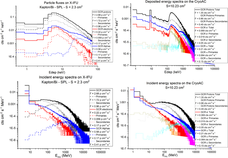
Figure 16. Top left: deposited energy spectra and integrated fluxes in the main detector (area = 2.3 cm2). Top right: deposited energy spectra and integrated fluxes in the CryoAC (Area = 10.23 cm2). Note that the primary particle spectra are flat below a certain energy and do not go to zero as expected. This is due to the fact that some particles have very short paths in the CryoAC pixels. Bottom panels: incident energy spectra on the two detectors, main detector (bottom-left panel, area = 2.3 cm2) and CryoAC (bottom right, area = 10.23 cm2); these energies are the ones possessed by the particles before interacting with the detectors. Note that the TES array detector area to be considered is the top surface, because the particle flux is to be compared to the source photon flux. The CryoAC area is the whole surface area (top + bottom + side) as it is the flux definition.
Download figure:
Standard image High-resolution imageWe expect on the main detector a total count rate from primary particles of 4.22 cts s−1. We require this component to impact the residual background by no more than 1/10 of the requirement, i.e., 5 × 10⁻⁴ cts cm−2 s−1 keV−1 in the 2–10 keV band, or 9.2 × 10⁻³ cts s−1. To reduce this flux down to the required level, we require a total rejection efficiency for primary particles of ∼99.78%. We remark here that the CryoAC rejection efficiency has to be calculated on the primary component, which is entirely rejectable and can be validated experimentally.
Analogously, we have a total count rate from secondary particles on the main detector of 2.75 cts s−1. However, a fraction of this flux is induced by unrejectable particles (i.e., electrons backscattering on the detector surface releasing just a fraction of their energy, low-energy particles that are completely absorbed inside the main array switching on only one pixel). The requirement on the rejection efficiency is placed on the rejectable component of the secondary particles flux, which amounts to 2.69 cts s−1. As for the primary case, we require this component to impact the residual background by no more than 1/10 of the requirement, 9.2 × 10⁻³ cts s−1. This sets the total rejection efficiency for rejectable secondary particles to ∼99.66%.
Now we start breaking down the X-IFU rejection efficiency by evaluating the geometrical contribution. An analysis has been performed on:
- 1.the CryoAC versus main detector related distance, and
- 2.the CryoAC area with respect to the main detector area.
We report the geometrical and total (geometrical + detector) rejection efficiencies in Figure 17. The results are related only to the primary component, which is entirely rejectable. Furthermore, to increase the statistics of the simulations, a reduced mass model of the instrument had to be created, and thus the secondary particle population, though not interesting for this analysis as stated above, impacting on the two instruments is not representative of the one experienced in the complete model.

Figure 17. Geometrical and total rejection inefficiency for primary particles (defined as the unity residual of the efficiency) as a function of the distance between the main detector and the CryoAC (left), and as a function of the CryoAC size increment with respect to the baseline size of 11.91 mm apothem (right). We show inefficiency rather than efficiency for clarity purposes.
Download figure:
Standard image High-resolution image
As can be seen in Figure 17, the geometrical rejection efficiency increases with the solid angle covered by the CryoAC. A 1.5 mm distance is enough to achieve the 99.78% total rejection efficiency goal. We adopt the 1 mm distance solution to account for some margin. Similarly, the baseline CryoAC size is sufficient to reach the goal (Figure 17, right), while further increase in the CryoAC size can be technically challenging and increase the instrument dead time, with minor benefits. The total rejection efficiency saturates beyond a given CryoAC size/distance, as we start discriminating events with very skewed trajectories, which are already intrinsically discriminated by the detector rejection efficiency.
Once the geometry of the system has been defined, we investigated the effect of the energy threshold of the CryoAC on its detection efficiency. We analyzed the residual background for the rejectable component (primary particles and secondaries). This is necessary because the primary component, despite being completely rejectable, constitutes a minor fraction of the residual background, so the secondary contribution cannot be ignored. We found that a 20 keV threshold fulfills the requirement. Lowering further the threshold value produces no appreciable benefit, while the unrejected background value starts to rise steeply above 30 keV.
Footnotes
- 5
R200 is defined as the radius within which the mean density is 200 times the critical density of the universe; M200 is the total mass enclosed within R200.
- 6
The SPL is available for download at the following URL: https://file.sic.rm.cnr.it/index.php/s/xsVgQnTtWG5Rbqq.