


Abstract
Many supernova remnants (SNRs), such as G296.5+10.0, exhibit an axisymmetric or barrel shape. Such morphologies have previously been linked to the direction of the Galactic magnetic field, although this remains uncertain. These SNRs generate magnetohydrodynamic shocks in the interstellar medium, modifying its physical and chemical properties. The ability to study these shocks through observations is difficult due to the small spatial scales involved. In order to answer these questions, we perform a scaled laboratory experiment in which a laser-generated blast wave expands under the influence of a uniform magnetic field. The blast wave exhibits a spheroidal shape, whose major axis is aligned with the magnetic field, in addition to a more continuous shock front. The implications of our results are discussed in the context of astrophysical systems.
Export citation and abstract BibTeX RIS
1. Introduction
Magnetic fields are ubiquitous in the universe and may have an influence on any number of celestial objects as well as the medium between them (Han 2017). The magnetized interstellar medium (ISM) is stirred by many physical processes, such as coronal mass ejections (Richardson & Cane 2010), cloud–cloud collisions (Inoue & Fukui 2013), outflows from newly formed stars (Jimenez-Serra et al. 2004), shocks from stellar winds (Scoville & Burkert 2013) and supernova explosions (Uyaniker et al. 2002; Gent et al. 2013). In many of these processes, magnetic fields play an important and often integral role.
For example, a subclass of supernova remnants (SNRs) exhibit a barrel (also called bilateral or axisymmetric) shape (Balsara et al. 2001; West et al. 2016)(see, for example, G296.5+10.0; Vasisht et al. 1997; Harvey-Smith et al. 2010). On the one hand, Van der Laan (1962) was the first to propose that an SNR expanding in a relatively uniform magnetic field would sweep up and compress the field where the expansion is perpendicular to the field lines. Regions with a higher field strength would subsequently produce higher intensity radio synchrotron emission and would thus lead to the formation of the bright limbs that are seen in observations (Giacani et al. 2000). On the other hand, although it is expected that magnetic fields influence SNRs on some level (Chevalier 1974), some studies have argued that the primary cause for these morphologies is the inhomogeneous ISM (Kesteven & Caswell 1987) or gradients in ambient density (Orlando et al. 2007). If the former explication is correct, then the orientation of SNRs would be an excellent tracer of the direction of the Galactic magnetic field (GMF; Whiteoak & Gardner 1968).
There have been many theoretical studies on the physical structure of magnetohydrodynamic (MHD) shocks on a smaller scale. The existence of magnetic precursors along with continuous density profiles across the shock front have been predicted in the presence of a strong transverse magnetic field (Draine 1980; Chieze et al. 1998). Other studies have proposed modified 1D Rankine–Hugoniot equations for the shock front with various different magnetic field configurations (Shu 1991). Many subsequent astrophysical studies rely on these theoretical predictions in order to explain certain observations (Jiménez-Serra et al. 2009), although these models are currently poorly constrained. Significant progress has been made recently, with observations using the Atacama Large Millimeter/submillimeter Array detecting spatially resolved MHD shocks for the first time (Cosentino et al. 2019). However, discrepancies exist between theoretical predictions and observational data, with the authors suggesting that MHD shock theory may need to be revisited.
We have thus far only considered the effect of magnetic fields on material dynamics. However, the processes discussed above naturally influence and change the nature of the magnetic field themselves. One example of this is amplification of magnetic fields by the turbulent dynamo process (Tzeferacos et al. 2018). In other words, magnetic fields affect material dynamics, but material dynamics also affect magnetic fields (Draine 1980). This means that any astrophysical model must treat these two self-consistently if it hopes to be successful (Shu 1991).
It is therefore of utmost importance to measure the value of the GMF as well as the magnetic field strength around celestial objects and in the ISM. However, we cannot directly measure the magnetic fields of these objects in situ. The techniques we use to measure magnetic fields, such as Faraday rotation or radio synchrotron emission are instead integrated along the line of sight of the telescope and blurred out due to a limited spatial resolution (Zeldovich et al. 1983; Kronberg 1994; O'Dea et al. 2011; Ade et al. 2016). In reality, magnetic fields in most emission regions are not well ordered, and they consist of small-scale irregular fields and large-scale Galactic ordered fields. Because irregular fields dominate interstellar space, it is sometimes hard to uniquely determine magnetic field structures from observations (Han 2017).
Experiments using high-power lasers can recreate aspects of astrophysical phenomena in the laboratory, allowing the creation of experimental platforms where observations and models can be quantitatively compared with data taken in a controlled laboratory environment (Remington et al. 1999). Laser-generated blast waves have been studied as analogs to SNRs for many years (Edwards et al. 2001); however, testing the effects of magnetic fields has remained out of reach. With recent technological advances, substantial volumes of astrophysically relevant magnetized plasmas can now be produced in the laboratory (Albertazzi et al. 2013). Studies have been performed to investigate expanding volumes of plasma (Collette & Gekelman 2010; Bonde et al. 2018), diamagnetic bubbles (Niemann et al. 2013), accretion columns (Albertazzi et al. 2018; Mabey et al. 2019), interpenetrating plasma flows (Shaikhislamov et al. 2015), and particle dynamics in collisionless shocks (Schaeffer et al. 2017, 2019). Nevertheless, many topics, such as the structure of MHD shocks, the energy partitioning between electrons and ions across collisionless shocks, or the propagation of SNRs through a magnetized ISM, still remain poorly understood.
In this paper, we present the laboratory observation of a laser-produced plasma blast wave expanding in a uniform magnetic field. Our results provide further evidence to support the existence of a magnetic precursor ahead of the shock front as well as highlighting the importance of taking the magnetic field into account when modeling expanding SNRs or other nonstationary shock waves.
2. Experimental Setup
The experiment was performed on the LULI laser facility and is shown schematically in Figure 1. A 45 J, 1 ns, 527 nm drive laser was focused to a focal spot of 250 μm onto a 300 μm cylindrical graphite pin. The target chamber was filled with 11.4 mbar of nitrogen gas, leading to the generation of a blast wave upon ablation of the pin (Albertazzi et al. 2020). Time-resolved schlieren images, as well as the self-emission from the blast wave, streaked in time, were recorded. For the latter, a long-pass filter was used to shield the camera from the laser light, allowing only wavelengths above 580 nm to be detected. Time-resolved optical spectroscopy was employed in the 450-800 nm range. Data were taken over a small volume (200 × 200 × 400 μm) at various distances between 1.5 and 2.4 mm away from the target, in the direction of the laser axis. These distances were sufficiently far away from the laser-plasma interaction so as to prevent any significant amount of carbon ablated from the target from entering the detector's field of view. The entire experimental setup was placed in a coil that was driven by a pulsed power machine in order to create a spatially uniform magnetic field of 10.2 T (Albertazzi et al. 2018; Mabey et al. 2019). The magnetic field remains constant (less than 2% variation) for a period of several microseconds, much larger than the timescales considered in this experiment.
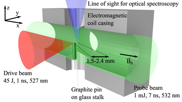
Figure 1. Experimental setup at the LULI2000 laser facility. The drive laser is focused down onto a graphite pin, creating a spherically expanding blast wave in the ambient nitrogen gas. A probe laser, propagating in the transverse direction (x), is used to take 2D Schlieren images. Self-emission is also recorded along this direction. Optical spectroscopy is recorded in the z direction at distances between y = 1.5 and 2.4 mm from the laser focus. Only a cutaway of the casing for the electromagnetic coil is shown for the sake of visual clarity. The coil is aligned such that the generated magnetic field, B0, runs parallel to the probe beam.
Download figure:
Standard image High-resolution image3. Results
Experimental data are displayed in Figures 2–7. The time-resolved emission spectroscopy images are shown in Figure 2. Spectra taken at the moment the blast wave passed through the line of sight of the detector were compared with 100 PRISMSpect (MacFarlane et al. 2007) simulations in order to determine the temperature and density of the plasma. This was achieved by finding a best fit of the simulated peak ratios and line widths, as demonstrated in Figures 2(c) and (d). For the 10.2 T case at 1.5 mm from the laser focus, values of T = 3.8 ± 0.7 eV and ρ = (3 ± 1)×10−5 g cm−3 were found, corresponding to a density compression ratio of ∼ 2. A similar analysis for the 0 T case found values of T = 3.8 ± 0.7 eV and ρ = (6 ± 1) × 10−5 g cm−3, corresponding to a density compression ratio of ∼ 4: as would be expected in the case of a purely hydrodynamic strong shock. Figure 3 shows 2D schlieren images of a segment of the blast wave without and with a perpendicular B0 = 10.2 T magnetic field. Figure 4 displays lineouts representing the 1D density gradient profile across the blast wave shock front as taken from the schlieren images. Streaked 1D self-emission data for the three cases of no magnetic field as well as perpendicular and parallel magnetic fields of 10.2 T are shown in Figure 5. The profile of the nitrogen line at 568 nm taken from the emission spectroscopy data is given in Figure 6 in order to demonstrate the profile of the shock front. Finally, Figure 7 displays the width of the blast wave shell at different angles with respect to the magnetic field.
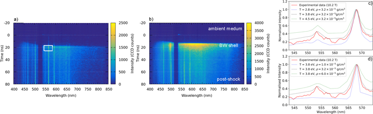
Figure 2. Streaked spectroscopy data at a distance of 1.5 mm from the laser focus in the case of (a) a perpendicular magnetic field of 10.2 T and (b) no applied magnetic field. A line filter centered on 527 nm was used to prevent any stray laser light reaching the detector. Panel (c) shows a sample section of the spectrum taken from (a) together with three PrismSPECT simulations of different densities. The ratios of the line widths are used to determine the best fit. Panel (d) shows the same experimental data together with three simulations of different temperatures, with the ratio of the peak intensities used to determine the best fit.
Download figure:
Standard image High-resolution image
Figure 3. Schlieren snapshots with and without the magnetic field at different delay times. Panels (a) and (b) show the image of the blast wave at 20 and 80 ns after the laser driver in the absence of the magnetic field. The width and the radius of the blast wave are well defined. Panels (c) and (d) show the corresponding data for the case of B0 = 10.2 T.
Download figure:
Standard image High-resolution image
Figure 4. Lineouts taken across the blast wave shell from schlieren images, with and without magnetic field, at 10, 50, and 100 ns, respectively. The distance scale is set such that the origin corresponds to the laser focus on the graphite target. The width of the blast wave shell is measured by taking the FWHM of the peak in the Schlieren lineout and averaged over multiple shots with the same time delay, where possible.
Download figure:
Standard image High-resolution image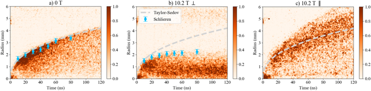
Figure 5. Streaked 1D self-emission data, taken at z = 0, for the three cases of (a) no magnetic field, (b) a 10.2 T magnetic field perpendicular to the direction of the propagation of the blast wave, and (c) a 10.2 T magnetic field parallel to the direction of propagation of the blast wave. The radius of the blast wave, as measured by the schlieren, is shown where possible. The trajectory predicted by ST theory is also displayed as a dashed gray line.
Download figure:
Standard image High-resolution image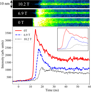
Figure 6. Raw data (top) and lineouts (bottom), showing the evolution of the nitrogen emission line at 568 nm as a function of time at 1.5 mm from the target for three magnetic field strengths. The rise in intensity of this line corresponds to the arrival of the blast wave into the line of sight of the diagnostic. The inset shows a magnified section between 10 and 25 ns. The transition from a sharp peak to a flatter line demonstrates the increasing continuous nature of the shock front with increasing magnetic field strength.
Download figure:
Standard image High-resolution image
Figure 7. Panel (a) shows three lineouts taken across the blast wave shell from schlieren images as a function of the azimuthal angle ϕ. The subsequent width of the shell is plotted in panel (b), with a maximum evident at ϕ = 90. The data correspond to the case of B = 10.2 T at a delay of 50 ns with respect to the laser drive.
Download figure:
Standard image High-resolution image3.1. Departure from Spherical Symmetry
It is clear that the magnetic field has a significant impact on the behavior of the blast wave, with both its shell width, d, and its radius, r, strongly affected. In the absence of a magnetic field, the radius, as measured by both diagnostics, increases with time, t, following the usual Sedov–Taylor (ST) law (Taylor 1950):
where E0 is the initial energy of the blast wave and ρ0 is the initial density of the ambient gas. When a perpendicular magnetic field is introduced, however, the rate of deceleration increases, beyond what is predicted by conventional ST theory. This phenomenon is seen across all diagnostics. The SOP images as well as the schlieren images and lineouts all show the radius of the shell segment increase initially before stalling around 2 mm from the target. Further evidence of this phenomenon may also be seen through the spectroscopy data. Figure 6 shows the evolution of the nitrogen emission line, at 568 nm at 1.5 mm from the target, as a function of time. The increase in intensity of this line, corresponding to the arrival of the shock, is delayed as the field strength is increased.
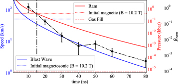
In order to understand the blast wave dynamics, we begin by examining the assumptions made by the ST model. We proceed by considering the relative pressures present in the system, as shown in Figure 8. For a given shock speed, vs, the ST model assumes that the ram pressure,  , is much larger than the ambient pressure of the medium into which the blast wave propagates, P0. The ram pressure of the blast wave as it is launched, Pram ∼ 1 kbar, is many orders of magnitude above the thermal pressure of the ambient nitrogen gas fill, P0 ∼ 11.4 mbar. By taking the derivative of the radius with respect to time and squaring, one notes that the pressure of the blast wave within the ST model decreases as, Pram ∝ t−6/5. In spite of this, it remains much larger than the ambient pressure over the 100 s of ns timescales considered here. The radiation pressure may also be calculated within the blackbody approximation. In reality this represents an upper bound on the real radiation pressure and may be written as,
  , where σ is the Stefan–Boltzmann constant and c is the speed of light. Taking the experimentally measured value for T, we find a value of Prad ∼ 5 mbar; also negligible compared to the ram pressure of the shock.
Figure 8. Evolution of the speeds and pressures in the blast wave as a function of time. Pram, PB, and vms are calculated using the formulae in the text. The self-emission image shown in Figure 3 is used to determine vs as a function of time while the optical spectroscopy measurement of ρ = (3 ± 1)×10−5 g cm−3 is used as the density. The circular markers correspond to values of βram, calculated using the shell width and radius at 10–20 ns intervals using the schlieren images.
Download figure:
Standard image High-resolution image
On shots where the magnetic field is turned on, an additional pressure is introduced into the system,  , where μ0 is the permeability of free space. The values for the magnetic field strengths here are PB (6.9 T) = 0.2 kbar, and PB (10.2 T) = 0.4 kbar respectively. The magnetic pressure is therefore much larger than the thermal pressure of the ambient gas and importantly, is of a similar order of magnitude to the ram pressure of the shock. The ratio of the ram pressure to the magnetic pressure is defined as
  . Initially, (
 ns)
ns)  , and hence the propagation of the blast wave follows the purely hydrodynamic case. However, as the ram pressure of the blast wave decreases, at some time later (t ∼ 15 ns), the magnetic pressure becomes dynamically significant (βram approaches unity). This causes the trajectory to deviate from that predicted by the ST model. A positive feedback loop is created, whereby, as the magnetic field causes Pram to decrease, the relative importance of the magnetic pressure increases and hence Pram decreases even further. This is shown explicitly in Figure 8 through the rapid decrease in βram between 10 and 40 ns.
We consider the magnetic Reynolds number of the plasma, the ratio of the magnetic advection to diffusion,  , where U and L are the typical velocity and length scales and η is the magnetic diffusivity (Ryutov et al. 2000). This parameter determines the extent to which magnetic field lines follow the flow of the plasma. Taking the formula η (cm2 s−1)
 ![$=1.5\times \,{10}^{7}\,Z\,/\,{[T(\mathrm{eV})]}^{3/2}$](https://content.cld.iop.org/journals/0004-637X/896/2/167/revision1/apjab92a4ieqn8.gif) (Braginski 1965), together with values of T = 3.8 eV and Z =1.8, allows us to calculate the magnetic diffusivity. For the length and velocity scales, we take the blast wave radius and speed, respectively. Taking the values at 50 ns, we have characteristic scales of U = 20 km s−1 and L = 2 mm, and thus an estimated value of Rm ∼ 1. These parameters of course vary as the blast wave expands and decelerates, and hence so does Rm. The modest value obtained here suggests that the frozen-in flux approximation cannot be applied unilaterally. Although diffusion is nonnegligible, the passing of the blast wave may distort the previously uniform magnetic field to some degree, compressing and bending the field lines. In this case, the magnetic pressure acts to counter this compression. As the blast wave propagates, it decelerates and the associated ram pressure decreases. Thus the degree to which the blast wave is able to compress the field lines also decreases. As a result, the blast wave's propagation is hindered and it decelerates further, causing a positive feedback loop, until at some distance, it stops entirely and dissipates (see Figure 3(d)).
(Braginski 1965), together with values of T = 3.8 eV and Z =1.8, allows us to calculate the magnetic diffusivity. For the length and velocity scales, we take the blast wave radius and speed, respectively. Taking the values at 50 ns, we have characteristic scales of U = 20 km s−1 and L = 2 mm, and thus an estimated value of Rm ∼ 1. These parameters of course vary as the blast wave expands and decelerates, and hence so does Rm. The modest value obtained here suggests that the frozen-in flux approximation cannot be applied unilaterally. Although diffusion is nonnegligible, the passing of the blast wave may distort the previously uniform magnetic field to some degree, compressing and bending the field lines. In this case, the magnetic pressure acts to counter this compression. As the blast wave propagates, it decelerates and the associated ram pressure decreases. Thus the degree to which the blast wave is able to compress the field lines also decreases. As a result, the blast wave's propagation is hindered and it decelerates further, causing a positive feedback loop, until at some distance, it stops entirely and dissipates (see Figure 3(d)).
Thus far, we have limited our discussion to segments of the blast wave, which propagate perpendicular to the magnetic field. However, since the initial expansion is isotropic, there are segments where the magnetic field is parallel to the propagation of the blast wave. Figure 5(c) shows that such segments decelerate at a slower rate than what would be expected in the absence of a magnetic field (i.e., it travels faster than predicted by ST theory). The net result is that the blast wave becomes a prolate spheroid as it propagates, with the major axis aligned along the magnetic field. We also note that the volume of said spheroid is lower than the sphere obtained in the absence of a magnetic field.
3.2. Toward a Continuous Shock Front
The magnetic field also influences the nature of the shock front itself. Figure 4 shows a relatively thin shell structure at early times, which widens in the presence of the magnetic field as the blast wave propagates. Again, the optical spectroscopy data provide corollary evidence for this effect. When no field is present, the increase in intensity of this line is sharp, corresponding to the arrival of a discontinuous heated shock front. As the field becomes stronger, the increase in intensity becomes more gradual, pointing to the arrival of a more continuous temperature gradient. Thus, the introduction of the magnetic field causes the shock front to transition from a discontinuous to a continuous state, both in terms of the density and temperature profiles.
This transition is best explained by considering the various characteristic speeds within the system (Draine 1980; see Figure 8). Compressive acoustic waves can propagate at the sound speed  Meanwhile MHD waves may propagate parallel to the magnetic field with the Alfvén speed
  , leading to the definition of the Alfvénic Mach number,
  . Here, the restoring force is provided by tension in magnetic lines. More relevant to our discussion are magnetosonic waves that propagate perpendicular to the field lines. In this case, the speed is given by
  As B → 0, the Alfvén velocity vanishes and the magnetosonic waves become regular acoustic waves. In the absence of a magnetic field, in order to have a discontinuous or jump (J) shock, one requires that vs > cs. It follows then that in the presence of a magnetic field, as the preshock medium is able to communicate compressive disturbances over long distances at the speed vms, one instead requires vs > vms. When vms > vs, the upstream medium (a partially ionized plasma with nonnegligible ion and neutral populations; Albertazzi et al. 2020) may be disturbed by magnetosonic waves, which travel faster than the shock. As they are damped by the neutrals, the preshock magnetic field is compressed, thereby also heating and compressing the medium prior to the arrival of the shock front. This causes a departure from a discontinuous or jump (J) shock and toward a continuous (C) shock. Such an effect has been invoked to interpret observations (Chieze et al. 1998; Jiménez-Serra et al. 2009) as well as experimental data (Schaeffer et al. 2019), but direct observation in the laboratory has remained elusive. Taking the initial magnetic field of 10.2 T, we calculate vms ∼ 50 km s−1. We therefore have a scenario where, initially vs > vms, leading to the thin shell structure observed. However, as the shock decelerates, these two speeds become similar and so the transition from a J-shock to a C-shock is observed. The time at which this occurs is very similar to the time at which the blast wave deviates from an ST trajectory, as expected. The data also permit the study of the width of the shell as a function of the azimuthal angle, ϕ, defined as the angle between the initial magnetic field and the radius vector of a given shell segment. As expected, the data, shown in Figure 7, show that the width is maximal at ϕ = 90, i.e., when the magnetic field is exactly perpendicular. The width is approximately constant for ϕ < 60, suggesting that the perpendicular component of the magnetic field at such angles is not sufficient to affect the shock structure. Although of interest, no data is available for the parallel field configuration (ϕ = 0) at this time. Further experiments would therefore be required in order to study the physics of the shock in the polar regions.
3.3. Magnetic Field Compression
As discussed previously, it is of significant astrophysical interest to calculate the increase in magnetic field as it is compressed by a passing shock wave (Völk et al. 2005). Although no dedicated magnetic field diagnostics were deployed in this experiment, the data nevertheless permit us to make an estimate based on the observations. The first method we propose assumes that all the magnetic flux is swept up by the blast wave. This is undoubtedly an overestimation given the modest (compared to astrophysical systems) magnetic Reynolds number. To proceed, we consider the conservation of flux in the blast wave shell, from which one can show that the magnetic field is equal to (Van der Laan 1962):
Taking the measured experimental values, as shown in Figure 3, we find values of B (10 ns) = 24 ± 3 T, B (50 ns) = 19 ± 5 T, and B (100 ns) = 16 ± 5 T. The magnetic field initially increases as the radius of the shell expands, before decreasing again as the width of the shell becomes larger. This suggests an intermediate time exists where the magnetic field reaches its peak value before relaxing back toward its initial value. Here the maximum amplification factor is found to be χ = B/B0 ∼ 2.4. One notes that, like the ST solution, this simple formula breaks down as t → 0. As an aside, we note that the magnetic field amplification factor here, determined from the shell width as measured by the schlieren diagnostic, is consistent with the density compression ratio of ∼2, as measured from the optical spectroscopy, giving us confidence in our data analysis methods.
One may also determine the magnetic field within the blast wave shell by considering the jump conditions across the shock front. It can be shown that the conservation of momentum leads to the following equation (Shu 1991)

where the subscripts (1, 0) refer to the postshock and preshock regions, respectively. Using the plasma parameters taken from the optical spectroscopy analysis, and assuming an ideal equation of state in order to determine P, we have all that is required to estimate the magnetic field in the postshock region at t ∼ 50 ns. We find a value of B1 = 14 T, which, although smaller than the value calculated using the conservation of flux method, is still within the estimated experimental error. The relative agreement between these two entirely separate approaches gives us good confidence in this result and validates the frozen-in flux approximation used in the former. Future experiments may measure the magnetic field directly via induction probes (White et al. 2019), Faraday rotation (Oliver et al. 2017), or Zeeman splitting (Liu et al. 2019).
4. Discussion
Our results provide physical evidence to support the argument that bilateral SNR morphologies may be caused by uniform ambient magnetic fields, at least when  . We take, as a case study, G296.5+10.0 (see Table 1), which represents a well-defined axisymmetric SNR.8
Despite the striking nature of the images, the mechanism responsible for the observed barrel-shape morphology remains unclear. Giacani et al. (2000) argued against the existence of a particular alignment of high-density regions in the interstellar gas being responsible, while not ruling out a magnetic-based explanation. Following on from this, Harvey-Smith et al. (2010) concluded that the observed rotation measure (RM = 40 rad m−2) from the SNR could not be caused by an ambient uniform magnetic field, favoring instead a radial field generated by a progenitor star. According to their prediction, such a uniform field ought to produce a much higher rotation measure, RM = 130–260 rad m−2. Their calculation assumes that the SNR is in the ST phase of its evolution (Roger et al. 1988), implying a density compression ratio of 4 and a shell thickness, d = r/12. However, a dynamically significant magnetic field would invalidate this assumption and thus the approach is not self-consistent.
. We take, as a case study, G296.5+10.0 (see Table 1), which represents a well-defined axisymmetric SNR.8
Despite the striking nature of the images, the mechanism responsible for the observed barrel-shape morphology remains unclear. Giacani et al. (2000) argued against the existence of a particular alignment of high-density regions in the interstellar gas being responsible, while not ruling out a magnetic-based explanation. Following on from this, Harvey-Smith et al. (2010) concluded that the observed rotation measure (RM = 40 rad m−2) from the SNR could not be caused by an ambient uniform magnetic field, favoring instead a radial field generated by a progenitor star. According to their prediction, such a uniform field ought to produce a much higher rotation measure, RM = 130–260 rad m−2. Their calculation assumes that the SNR is in the ST phase of its evolution (Roger et al. 1988), implying a density compression ratio of 4 and a shell thickness, d = r/12. However, a dynamically significant magnetic field would invalidate this assumption and thus the approach is not self-consistent.
Table 1. Scaling between the Laboratory Experiment Described in This Work and SNR G296.5+10.0
| Laboratory | G296.5+10.0 | |
|---|---|---|
| Radius | 1.5 mm | 20 pc |
| Velocity | 100 km s−1 | 1800 km s−1 |
| Age | 10 ns | 10,000 yr |
| Initial density | 3 × 1017 cm−3 | 0.1 cm−3 |
| Magnetic field | 10.2 T | 240 μG |
| Temperature | 3.8 eV | 150 eV |
| βram | 2 | 2 |
| Rm | 1 | 1024 |
| MA | 1 | 1 |
Note. For the former, the values represent a given snapshot in time, as, in general, they evolve over the course of the experiment. The values for the astrophysical case are cited within the text, except for the temperature, which is taken from Holland-Ashford et al. (2017).
Download table as: ASCIITypeset image
To compare to our results, we seek to calculate βram for the astrophysical case. The velocity of the SNR may be estimated within ST theory by taking a standard supernova explosion energy of 1051 erg, an initial density of 0.1 cm−3 (Matsui et al. 1988), and an age of 10,000 yr (Halpern & Gotthelf 2015), giving vs = 1800 km s−1. Recent studies have suggested that the magnetic field strength within the shell could be as high as B = 240 μG (Araya 2013), which would give a value of βram ∼ 2. This is a similar value of βram to our experiment and thus we would expect to see significant deviations from ST theory in the behavior of SNR G296.5+10.0. Moreover, our results indicate a density compression ratio of ∼2 as well as a ratio of d/r = 1/6 would be expected. There is also observational evidence for a more continuous shock front in the presence of a moderate βram and so we conclude that a compression ratio of 4 in the case of SNR G296.5+10.0 is unlikely. These factors would decrease the predicted value of RM, bringing it within observational error. We therefore favor the explanation supported by West et al. (2016), Roger et al. (1988), and Milne (1987), that a large-scale uniform ambient magnetic field is responsible for the observed morphology. Finally, it is worth noting that G296.5+10.0 is not a particularly old SNR. That is to say, its expansion velocity has not yet decreased to the point at which radiative effects are significant enough to cause the blast wave to enter the so-called snowplow regime (∼ 150 km s−1) (Ostriker & McKee 1988). If other SNRs deviate from spherical symmetry before radiative losses become important, the subsequent decrease in volume of the SNR shells would also lead to a lower star formation rate (Cioffi et al. 1988), although this requires further study.
5. Conclusions
In summary, we have shown that a blast wave propagating in a dynamically significant magnetic field will depart from spherical symmetry. Segments perpendicular to the field will undergo an increased deceleration while segments parallel to the field will decrease at a slower rate. The blast wave thus sweeps out a spheroidal shape in space, with the major axis aligned along the direction of the magnetic field. The ambient magnetic field increases initially as it is compressed by the passing of the shock. As the ram pressure of the blast wave decreases, the width of its shell increases, with the shock front exhibiting a transition from a J-type to a C-type, thus also causing the magnetic field to relax back toward its initial value. These results provide strong evidence for the connection between bilateral SNRs and the GMF as well as providing an ideal platform to study MHD shock theory in a controlled environment. Experiments such as this one provide a potential route to answering many outstanding questions surrounding celestial magnetic fields.
The authors would like to thank all of the staff at the LULI laser facility for their great support in obtaining the results presented in this paper. The work of C.A.J.P., J.T.-M., and G.G. was supported in part by the UK Engineering and Physical Sciences Research Council (grant Nos. EP/M022331/1 and EP/N014472/1).