


Abstract
The aim of this paper is to investigate the effect of rotation on the single and binary evolution for Population III stars. A small grid for a massive Population III star of 130 M⊙ is constructed, and various initial conditions are adjusted to explore the evolution. For comparison, we present the evolution of the models with the metallicity in the Small Magellanic Cloud and analyze the characteristic feature of chemically homogeneous evolution. It is found that Population III stars attain the equilibrium velocities later during synchronization owing to a smaller radius. The equilibrium velocity has been expressed as various timescales. There appears to be a deep dredge-up at hydrogen exhaustion for single Population III stars. It not only increases the helium core but also exchanges chemical elements between the He core and the H-burning shell. This will give rise to a significant amount of nitrogen and neon. Rotational mixing can reduce the specific entropy in the envelope and increase the specific entropy in the core owing to a change of mean molecular weight. Stellar compactness and the luminosity available for stellar expansion are decreased by rotational mixing because of the increase of helium in the envelopes. Mass loss induced by strong stellar winds and Roche lobe overflow can extinguish the hydrogen-burning shell and remove convective envelopes. Therefore, this process does not favor the dredge-up and production of primary nitrogen. The chemical structure for two components in binarities is significantly modified because Roche lobe overflow has an impact on convective cores.
Export citation and abstract BibTeX RIS
1. Introduction
The first generation of stars in the universe are called Population III stars. These stars have formed at a redshift of Z ≃ 15–20 out of primordial gas, composed of about 75% hydrogen and ∼25% helium, with only a tiny amount of lithium and deuterium (Bromm et al. 2009). These first stars are thought to be very massive, and they have ended the epoch of the so-called "dark age" at about 200 million years after the recombination time (Bowman et al. 2018). This composition leads to special features in their structure and evolution. Population III stars play a key role in the history of the universe, as a link between the pure H–He universe at the beginning of times and the metal-rich one that we have observed nowadays around us. These stars with very low heavy-element abundances are of great importance for two reasons. First, they contribute to reionization of the universe through their energetic radiation. Second, their nucleosynthetic yields are the seeds for the makeup of later generations of stars and galaxies. It is significant to predict the final fate of Population III stars because they were the first producers of heavier elements and chemically enriched the universe through explosions and stellar winds. Direct identification of Population III stars will be highly impossible even with high-resolution telescopes. However, observational investigations on the surface abundances of extremely metal-poor stars, which are believed to retain the nucleosynthesis signatures of Population III stars, will also provide a good constraint on the evolution of Population III stars.
Stacy et al. (2011) have indicated that it is very probable that Population III might have had high rotational velocities close to the critical value. Rotation can trigger various instabilities insider the star. Redistribution of angular momentum and chemical species then proceed as a consequence of Eddington–Sweet circulation, Solberg–Høiland instability, the Goldreich–Schubert–Fricke instability, and secular and dynamic shear instability (Heger et al. 2000; Heger & Langer 2000; Maeder & Meynet 2000, 2012; Langer 2012). Among them, meridional circulations and shear turbulences can transport both angular momentum and chemical species, which can significantly modify the structure and evolution of stars (Talon & Zahn 1997; Maeder & Zahn 1998; Meynet & Maeder 2000). Rotation may also affect the mass-loss rate of stellar winds through surface enrichment and the centrifugal force (Langer 1998; Maeder et al. 2005; Meynet et al. 2005). Therefore, it can influence the final fate of a star (Yoon et al. 2008, 2012). At least a fraction of the first stars could have collapsed into massive black holes at the end of their short lives, thus providing viable gamma-ray burst progenitors (Toma et al. 2016).
During recent years, many investigations have been carried out on the evolution and possible final fates of Population III stars (Heger & Woosley 2002; Limongi & Chieffi 2012; Dessart et al. 2013; Whalen et al. 2013). The Population III generation of stars was believed to be intrinsically massive, with masses ranging from 30 to 1000 times that of the Sun. Nonrotating models without mass loss were computed by Marigo et al. (2001) and Heger & Woosley (2002), who covered a large range of mass (Mini = 0.7–1000 M⊙). In a follow-up paper Heger & Woosley (2002) studied the evolution of nonrotating helium stars and focused on the resulting nucleosynthetic imprints and pair-instability supernovae. Ekström et al. (2008) computed grids of Population III stars with rotation. They found that mass is lost in particular when the models attain critical rotation. The cores of their models all reached a very high angular momentum because of the weak coupling of core and envelope. The main reason is that Taylor–Spruit magnetic dynamo is absent in their models.
Almost all massive stars today are believed to be in binary systems (Sana et al. 2013). If the system is a close binary, one component can transfer mass to its companion star through Roche lobe overflow (RLOF). The theoretical model of binaries can be classified into two categories: either detailed evolutionary simulation, or population synthesis computations. These models have been discussed by De Marco & Izzard (2017), who listed the current state of binary evolution investigations. Several works have explored massive binaries by detailed evolutionary simulations (Yoon & Langer 2005; Yoon et al. 2006; Cantiello et al. 2007; Marchant et al. 2016, 2017). On the other hand, many simulations have involved binary population synthesis (Podsiadlowski et al. 1992; Belczynski et al. 2002, 2016; Eldridge et al. 2008, 2011; Dominik et al. 2012, 2013). There are a growing number of theoretical binary evolutions for Population III stars. The evolution of Population III stars, including the effects of binary interaction, is described by Lawlor et al. (2008). Limongi & Chieffi (2012) have presented a grid of evolution models and obtained the nucleosynthetic yields during explosions for model masses between 13 and 80 M⊙.
In the present work, we aim to investigate how both rotation and binary systems can influence the structure and evolution of Population III stars. This work intends to uncover a number of differences between single and binary evolution for Population III stars. In particular, we want to explore how the combined effect of rotation and binary interactions has an impact on the nucleosynthesis and chemical structure for Population III stars. The paper is organized as follows: The initial parameters and model description are introduced in Section 2. In Section 3, the evolution and chemical structure of single and binary Population III systems are analyzed in detail. And finally, in Section 4, we summarize our conclusions and briefly discuss the effect of rotation on the evolution at the advanced burning stage.
2. The Initial Parameters and Model Descriptions
We have adopted the latest stellar evolution code MESA (Modules for Experiments in Stellar Astrophysics; version-r10398), which was originally written by Paxton et al. (2011, 2013, 2015), to compute our models. We particularly focus on the evolution during central hydrogen and helium burning. Please refer to the summary section for the detailed explanation.
The initial parameters adopted in our calculation are listed in Table 1. We set the initial orbital period to the value of RLOF when the following cases occur. Case A: the primary star fills its Roche volume during the main-sequence phase, and the corresponding orbital period is set to be 4.0 days. Case B: the primary star fills its Roche lobe after core H exhaustion, and the corresponding orbital period is set to be 7.6 days. Case C: the primary star fills its Roche lobe during core He burning, and the corresponding orbital period is set to be 13.0 days.
Table 1. Parameters Adopted in Our Calculations
| Models |

|

|

|

|

|

|

|
Z | CC |

|
|---|---|---|---|---|---|---|---|---|---|---|
| (M⊙) | (M⊙) | (km s−1) | (km s−1) | (days) | ||||||
| S1 | 130 | ⋯ | 0 | ⋯ | ⋯ | ⋯ | 0.0228 | 10−14 | Led. | 0 |
| S2 | 130 | ⋯ | 0 | ⋯ | ⋯ | ⋯ | 0.0228 | 10−14 | Sch. | 0.25 |
| S3 | 130 | ⋯ | 0 | ⋯ | ⋯ | ⋯ | 0.0228 | 10−8 | Sch. | 0.25 |
| S4 | 130 | ⋯ | 0 | ⋯ | ⋯ | ⋯ | 0.0228 | 0.0021 | Led. | 0 |
| S5 | 130 | ⋯ | 0 | ⋯ | ⋯ | ⋯ | 0.0228 | 0.0021 | Sch. | 0.25 |
| S6 | 100 | ⋯ | 0 | ⋯ | ⋯ | ⋯ | 0.0228 | 10−14 | Led. | 0 |
| S7 | 100 | ⋯ | 0 | ⋯ | ⋯ | ⋯ | 0.0228 | 10−14 | Sch. | 0.25 |
| S8 | 130 | ⋯ | 600 | ⋯ | ⋯ | ⋯ | 0.0228 | 10−14 | Sch. | 0.25 |
| S9 | 130 | ⋯ | 600 | ⋯ | ⋯ | ⋯ | 0.0228 | 10−8 | Sch. | 0.25 |
| S10 | 130 | ⋯ | 800 | ⋯ | ⋯ | ⋯ | 0.0228 | 10−14 | Sch. | 0.25 |
| S11 | 130 | ⋯ | 600 | ⋯ | ⋯ | ⋯ | 0.0228 | 0.0021 | Sch. | 0.25 |
| S12 | 100 | ⋯ | 600 | ⋯ | ⋯ | ⋯ | 0.0228 | 10−14 | Sch. | 0.25 |
| B1 | 130 | 100 | 0 | 0 | 4.00 | 0.7 | 0.0228 | 10−14 | Sch. | 0.25 |
| B2 | 130 | 100 | 600 | 600 | 4.00 | 0.7 | 0.0228 | 10−14 | Sch. | 0.25 |
| B3 | 130 | 100 | 600 | 600 | 7.60 | 0.7 | 0.0228 | 10−14 | Sch. | 0.25 |
| B4 | 130 | 100 | 600 | 600 | 13.00 | 0.7 | 0.0228 | 10−14 | Sch. | 0.25 |
| B5 | 130 | 100 | 600 | 600 | 4.00 | 0.7 | 0.0228 | 10−8 | Sch. | 0.25 |
| B6 | 130 | 100 | 600 | 600 | 4.00 | 0.7 | 0.0228 | 0.0021 | Sch. | 0.25 |
| B7 | 130 | 100 | 600 | 600 | 1.90 | 0.7 | 0.0228 | 0.0021 | Sch. | 0.25 |
Note. The meaning of each column is as follows. The symbol S denotes single stars, whereas the symbol B denotes the evolution of the binary system.  : the initial mass of the primary star in units of M⊙;
  : the initial mass of the secondary star in units of M⊙;
  : the initial equatorial velocity of the primary star in units of km s−1;
  : the initial equatorial velocity of the secondary star in units of km s−1;
  : the initial orbital period;
  : the ratio of mass loss in the vicinity of the accretor to the total transferred mass; fc: the efficiency of rotationally induced mixing; Z: the metallicity; CC: convection criteria; αover: convective overshooting parameters; Led.: Ledoux convection; Sch.: Schwarzschild convection.
Download table as: ASCIITypeset image
Convection can efficiently mix chemical elements. Two different treatments of convection are adopted to investigate the dredge-up. The Ledoux criterion, which is combined with slow semiconvective mixing, is used. Slow semiconvective mixing is done according to the diffusive approach by Langer (1991), with the free parameter in this description set to 0.01. We also use the Schwarzschild criterion to determine the boundaries of the convective regions. In terms of the pressure scale height Hp, as the overshooting parameter is commonly defined in other stellar evolution codes, this value approximately compares to αover = 0.25. The energy transfer efficiency by convection is usually parameterized by the mixing length lm in units of Hp (i.e., lm = 1.5Hp).
According to the standard model of the big bang theory, the only elements the big bang could have produced are hydrogen, helium, and possibly a trace of lithium, but no other metals. Therefore, the first stars of the universe could have been made only from hydrogen and helium, and these stars are known as Population III stars. We would consider as Population III stars all massive stars with Z ≤ 10−10. The main reason is that massive stars cannot sustain their gravity with pp-chains; they rely on the CNO cycle, for which they need carbon. This is why they need to contract until they reach a central temperature that allows them to fuse a little bit of helium and produce some carbon. Then, they can launch the CNO cycle and evolve normally. Stars with an initial metallicity of Z = 10−14 can be considered as Population III stars, and the corresponding hydrogen and helium are set to be 0.765 and 0.235, respectively (Lawlor et al. 2015, 2008). In order to compare the evolution of stars at different metallicities, we also include the stars with a metallicity of Z = 10−8 and the stars with Z = 0.0021. The stars with a metallicity of Z = 10−8 approach the metallicity of Population III stars, and they represent the early star generations (Meynet et al. 2006). The stars with Z = 0.0021 represent the ones in the Small Magellanic Cloud. We intend to obtain a clear evolutionary tendency at different metallicities.
In a rotating star, the mixing process due to hydrodynamical instabilities in radiative regions is treated as diffusive processes according to Heger et al. (2000). The parameter fc is the efficiency of rotationally induced mixing, and it has been calibrated to reproduce the observed nitrogen surface abundances as a function of the projected rotational velocities for stars in the Large Magellanic Cloud sample (NGC 2004) of the FLAMES survey (Brott et al. 2011). We adopt  , which is calibrated by Yoon (2006).
We treated mass loss of stellar winds by the prescription of Vink et al. (2000, 2001), for both O- and B-type stars. This mass-loss formula predicts a fast increase of the mass-loss rate when the star shifts toward lower temperatures near 2.2 kK. This increase corresponds to the recombination of Fe iv to Fe iii at the sonic point and is commonly considered as the bi-stability jump. The increased mass loss at the second bi-stability jump at ∼12.5 kK has been accounted for in this paper. Also, mass loss has been included according to the prescription of de Jager et al. (1988) for the red supergiant phase (![${\rm{log}}{T}_{{\rm{eff}}}[K]\lt 3.8$](https://content.cld.iop.org/journals/0004-637X/892/1/41/revision1/apjab7993ieqn16.gif) ). When the helium surface abundance Ys exceeds the value of 0.7, we adopt the Wolf–Rayet (W-R) mass-loss rate, which is derived from Nugis & Lamers (2000). Mass loss is enhanced, in rapidly rotating stars, following the prescription of Heger et al. (2000). Thermohaline mixing can occur in accreting binaries when the gradient of molecular weight becomes negative
). When the helium surface abundance Ys exceeds the value of 0.7, we adopt the Wolf–Rayet (W-R) mass-loss rate, which is derived from Nugis & Lamers (2000). Mass loss is enhanced, in rapidly rotating stars, following the prescription of Heger et al. (2000). Thermohaline mixing can occur in accreting binaries when the gradient of molecular weight becomes negative  . This inversion of molecular weight is created by the accreted material, which contains heavy elements. The present model is computed adopting the prescription advocated by Charbonnel & Zahn (2007).
We employ the optically thick mass transfer prescription by Kolb & Ritter (1990) to calculate the mass transfer rate during RLOF. In this paper, we use βmt to denote the fraction of mass transferred that is lost from the vicinity of the accreting star. The efficiency of mass transfer is then given by fmt = 1.0 − βmt. Mass transfer plays a key role in binary evolution. In our calculation, we assume that mass is transferred from the donor star to the vicinity of the companion. Regarding nonconservative mass transfer (i.e., βmt = 0.7), a part of the transferred mass (i.e.,  ) that carries the specific orbital angular momentum of the mass gainer is directly expelled from the system. If the spin speed of the accretor does not attain the critical velocities, the remaining mass will be accreted onto the gainer. Once the accreting star attains critical velocities, the remaining mass will be deposited in an outer disk surrounding the accreting star. A tiny fraction of the mass of the disk compensates for the spin angular momentum loss that is carried away by the enhanced stellar winds. The enhanced stellar winds are predominately composed of the unbound matter induced by critical rotation, enabling the accretor to maintain subcritical rotation. Furthermore, radiation is present anyhow, and it progressively removes the matter from the stellar disk and dissipates the disk into the outer space.
In Table 2, we list the evolutionary age in units of Myr, stellar mass in units of M⊙, effective temperature  and corresponding luminosity
  , central temperature
  and corresponding central density
  , surface nitrogen abundance
 ![$[{\rm{N}}/{\rm{H}}]=\mathrm{log}({\rm{N}}/{\rm{H}})+12$](https://content.cld.iop.org/journals/0004-637X/892/1/41/revision1/apjab7993ieqn23.gif) , and equatorial velocities Veq in units of km s−1 at different evolutionary points of five models. In Table 3, we list surface various chemical elements in mass fraction for single stars at major evolutionary phases.
, and equatorial velocities Veq in units of km s−1 at different evolutionary points of five models. In Table 3, we list surface various chemical elements in mass fraction for single stars at major evolutionary phases.
Table 2. Major Evolutionary Parameters for Five Single-star Models
| Sequence | Age | M |

|

|

|

|

|
[N/H] |

|
|---|---|---|---|---|---|---|---|---|---|
| (Myr) | (M⊙) | (K) | (K) |

|
(km s−1) | ||||
| ZAMS | |||||||||
| S2 | 0.000 | 130.000 | 0.721 | 5.004 | 6.319 | 8.149 | 1.694 | −4.322 | 0 |
| S8 | 0.000 | 130.000 | 0.754 | 4.995 | 6.307 | 8.144 | 1.696 | −4.322 | 600 |
| S10 | 0.000 | 130.000 | 0.738 | 4.972 | 6.301 | 8.089 | 1.699 | −4.322 | 800 |
| S11 | 0.000 | 130.000 | 1.182 | 4.746 | 6.264 | 7.683 | 0.292 | 7.011 | 600 |
| S12 | 0.000 | 100.000 | 0.884 | 4.852 | 6.130 | 7.870 | 0.945 | −4.322 | 600 |
| TAMS | |||||||||
| S2 | 2.700 | 130.000 | 1.739 | 4.519 | 6.507 | 8.157 | 1.709 | −4.322 | 0 |
| S8 | 2.842 | 129.542 | 1.731 | 4.528 | 6.571 | 8.179 | 1.746 | 2.314 | 347 |
| S10 | 3.213 | 127.818 | 1.091 | 4.889 | 6.689 | 8.138 | 1.569 | 4.633 | 646 |
| S11 | 3.191 | 57.904 | 0.852 | 4.917 | 6.324 | 7.864 | 0.942 | 9.433 | 16 |
| S12 | 3.547 | 99.438 | 1.249 | 4.764 | 6.507 | 8.154 | 1.704 | 3.943 | 642 |
| BCHEB | |||||||||
| S2 | 2.704 | 130.000 | 1.679 | 4.552 | 6.522 | 8.328 | 2.228 | −4.322 | 0 |
| S8 | 2.845 | 129.541 | 1.702 | 4.555 | 6.576 | 8.335 | 2.221 | 2.314 | 458 |
| S10 | 3.216 | 127.788 | 1.008 | 4.933 | 6.700 | 8.335 | 2.166 | 4.637 | 970 |
| S11 | 3.196 | 57.536 | 0.437 | 5.134 | 6.364 | 8.305 | 2.268 | 9.467 | 44 |
| S12 | 3.550 | 99.364 | 1.169 | 4.806 | 6.517 | 8.326 | 2.226 | 3.945 | 750 |
| ECHEB | |||||||||
| S2 | 2.960 | 121.003 | 2.028 | 4.389 | 6.565 | 8.548 | 2.913 | 2.446 | 0 |
| S8 | 3.102 | 129.487 | 2.015 | 4.411 | 6.628 | 8.568 | 2.938 | 2.772 | 168 |
| S10 | 3.468 | 126.163 | 1.787 | 4.555 | 6.750 | 8.553 | 2.830 | 4.773 | 155 |
| S11 | 3.517 | 25.298 | 0.071 | 5.223 | 5.986 | 8.529 | 3.141 | 33.428 | 22 |
| S12 | 3.811 | 98.603 | 1.846 | 4.481 | 6.569 | 8.548 | 2.907 | 4.092 | 140 |
| BCCB | |||||||||
| S2 | 2.964 | 121.003 | 1.834 | 4.487 | 6.569 | 8.806 | 3.730 | 2.446 | 0 |
| S8 | ⋯ | ⋯ | ⋯ | ⋯ | ⋯ | ⋯ | ⋯ | ⋯ | ⋯ |
| S10 | 3.471 | 126.135 | 1.809 | 4.553 | 6.783 | 8.807 | 3.642 | 6.761 | 195 |
| S11 | 3.521 | 25.172 | −0.126 | 5.337 | 6.049 | 8.802 | 4.015 | 33.518 | 37 |
| S12 | 3.814 | 98.594 | 2.017 | 4.412 | 6.635 | 8.626 | 3.173 | 6.899 | 83 |
| EOC | |||||||||
| S2 | 2.964 | 121.003 | 1.805 | 4.502 | 6.571 | 8.954 | 4.379 | 2.446 | 0 |
| S8 | 3.103 | 129.487 | 2.002 | 4.418 | 6.630 | 8.623 | 3.106 | 2.773 | 180 |
| S10 | 3.471 | 126.124 | 1.857 | 4.542 | 6.836 | 9.146 | 4.996 | 7.479 | 199 |
| S11 | 3.521 | 25.161 | −0.317 | 5.441 | 6.082 | 9.092 | 5.353 | 33.282 | 51 |
| S12 | 3.814 | 98.594 | 2.017 | 4.412 | 6.635 | 8.626 | 3.173 | 6.899 | 83 |
Note. The abbreviations are as follows: ZAMS is zero-age main sequence; TAMS is the point of the terminal of core hydrogen burning; BCHEB is the point of the beginning of core helium burning; ECHEB denotes the point of the end of core helium burning; BCCB is the point of the beginning of core carbon burning; EOC represents the point of the end of calculation.
Download table as: ASCIITypeset image
Table 3. Surface Chemical Abundances for H, He, C, N, O, Ne, Mg, and Al in Mass Fraction for Single Stars at Selected Evolutionary Points
| Sequence | t(Myr), | M1/M⊙, |
 , , |
 , , |
 , , |
 , , |
 , , |
 , , |
 , , |
 , , |

|
|---|---|---|---|---|---|---|---|---|---|---|---|
| ZAMS | |||||||||||
| S2 | 0.000 | 130.000 | 0.765 | 0.235 | −14.763 | −15.293 | −14.324 | −15.007 | −16.099 | −16.379 | 0 |
| S8 | 0.000 | 130.000 | 0.765 | 0.235 | −14.763 | −15.293 | −14.324 | −15.007 | −16.099 | −16.379 | 0 |
| S10 | 0.000 | 130.000 | 0.765 | 0.235 | −14.763 | −15.293 | −14.324 | −15.007 | −16.099 | −16.379 | 0 |
| S11 | 0.000 | 130.000 | 0.746 | 0.252 | −3.440 | −3.970 | −3.002 | −3.685 | −4.777 | −5.057 | 1.47e−25 |
| S12 | 0.000 | 100.000 | 0.765 | 0.235 | −14.763 | −15.293 | −14.324 | −15.007 | −16.099 | −16.379 | 0 |
| TAMS | |||||||||||
| S2 | 2.700 | 130.000 | 0.765 | 0.235 | −14.763 | −15.293 | −14.324 | −15.007 | −16.099 | −16.379 | 0 |
| S8 | 2.842 | 129.542 | 0.603 | 0.397 | −10.423 | −8.760 | −10.322 | −14.608 | −17.852 | −16.615 | 1.51e−16 |
| S10 | 3.213 | 127.818 | 0.258 | 0.742 | −8.026 | −6.810 | −9.042 | −13.077 | −13.281 | −14.132 | 1.37e−15 |
| S11 | 3.191 | 57.904 | 0.034 | 0.964 | −4.234 | −2.885 | −4.650 | −3.771 | −7.422 | −8.283 | 6.10e−6 |
| S12 | 3.547 | 99.438 | 0.392 | 0.608 | −8.677 | −7.318 | −9.501 | −13.372 | −13.820 | −14.421 | 5.46e−16 |
| BCHEB | |||||||||||
| S2 | 2.704 | 130.000 | 0.765 | 0.235 | −14.763 | −15.293 | −14.324 | −15.007 | −16.099 | −16.379 | 0 |
| S8 | 2.845 | 129.541 | 0.603 | 0.397 | −10.423 | −8.759 | −10.322 | −14.607 | −17.853 | −16.615 | 1.51e−16 |
| S10 | 3.216 | 127.788 | 0.257 | 0.743 | −8.026 | −6.807 | −9.039 | −13.073 | −13.281 | −14.130 | 1.27e−15 |
| S11 | 3.196 | 57.536 | 0.032 | 0.966 | −4.232 | −2.885 | −4.653 | −3.772 | −7.419 | −8.238 | 6.10e−6 |
| S12 | 3.550 | 99.364 | 0.392 | 0.608 | −8.678 | −7.316 | −9.499 | −13.370 | −13.821 | −14.420 | 5.45e−16 |
| ECHEB | |||||||||||
| S2 | 2.960 | 121.003 | 0.576 | 0.424 | −10.145 | −8.648 | −10.328 | −14.355 | −17.374 | −17.056 | 2.38e−16 |
| S8 | 3.102 | 129.487 | 0.466 | 0.534 | −9.947 | −8.413 | −10.033 | −14.260 | −17.966 | −16.818 | 4.30e−16 |
| S10 | 3.468 | 126.163 | 0.231 | 0.769 | −8.167 | −6.717 | −8.739 | −12.940 | −13.459 | −14.129 | 3.30e−15 |
| S11 | 3.517 | 25.298 | 0.000 | 0.187 | −0.363 | −8.871 | −0.424 | −3.226 | −2.758 | −3.909 | 3.92e−16 |
| S12 | 3.811 | 98.603 | 0.349 | 0.651 | −8.719 | −7.219 | −9.173 | −13.274 | −14.006 | −14.456 | 1.48e−15 |
| BCCB | |||||||||||
| S2 | 2.964 | 121.003 | 0.576 | 0.424 | −10.145 | −8.648 | −10.328 | −14.355 | −17.374 | −17.056 | 2.66e−16 |
| S8 | ⋯ | ⋯ | ⋯ | ⋯ | ⋯ | ⋯ | ⋯ | ⋯ | ⋯ | ⋯ | ⋯ |
| S10 | 3.471 | 126.135 | 0.183 | 0.817 | −6.038 | −4.831 | −6.809 | −9.532 | −12.608 | −11.283 | 4.90e−12 |
| S11 | 3.521 | 25.172 | 0.000 | 0.180 | −0.368 | −8.843 | −0.411 | −3.205 | −2.760 | −3.887 | 4.37e−16 |
| S12 | 3.814 | 98.594 | 0.259 | 0.741 | −5.746 | −4.541 | −6.321 | −9.479 | −12.593 | −11.141 | 8.89e−12 |
| EOC | |||||||||||
| S2 | 2.964 | 121.003 | 0.576 | 0.424 | −10.145 | −8.648 | −10.328 | −14.355 | −17.374 | −17.056 | 2.37e−16 |
| S8 | 3.103 | 129.487 | 0.466 | 0.534 | −9.946 | −8.413 | −10.033 | −14.259 | −17.965 | −16.818 | 4.30e−16 |
| S10 | 3.471 | 126.124 | 0.173 | 0.827 | −5.265 | −4.138 | −5.772 | −8.664 | −11.017 | −10.280 | 1.51e−11 |
| S11 | 3.521 | 25.161 | 0.000 | 0.179 | −0.368 | −8.841 | −0.410 | −3.203 | −2.761 | −3.886 | 4.41e−16 |
| S12 | 3.814 | 98.594 | 0.259 | 0.741 | −5.746 | −4.541 | −6.321 | −9.479 | −12.593 | −11.141 | 8.89e−12 |
| BFDP | |||||||||||
| S10 | 3.0287 | 128.6982 | 0.4432 | 0.5568 | −10.0874 | −8.4351 | −10.0539 | −14.3049 | −16.4835 | −15.9325 | 3.13e−16 |
| S12 | 3.1677 | 99.9095 | 0.6266 | 0.3734 | −10.5949 | −8.8948 | −10.4552 | −14.7114 | −18.1917 | −17.3515 | 1.06e−16 |
| EFDP | |||||||||||
| S10 | 3.0288 | 128.6830 | 0.4394 | 0.5606 | −9.5413 | −8.1899 | −9.9885 | −14.2123 | −14.9129 | −15.6006 | 3.28e−16 |
| S12 | 3.1690 | 99.8839 | 0.6250 | 0.3750 | −10.3694 | −8.8058 | −10.4362 | −14.6603 | −15.8771 | −16.5148 | 1.08e−16 |
Note. The abbreviations are as follows: BFDP is the beginning of the first dredge-up; EFDP is the end of the first dredge-up. Other abbreviations are the same as in Table 2.
Download table as: ASCIITypeset image
In Table 4, we list the evolutionary age in units of Myr, orbital period Porb in units of days, mass of the donor star M1 and the accreting star M2 in units of M⊙, the central temperature for the donor star  and the corresponding central density
  , the effective temperature of the donor star
  and the corresponding luminosity
  , the effective temperature of the accreting star
  and the corresponding luminosity
  , the surface nitrogen abundance of the donor star
 ![$[{{\rm{N}}}_{1}/{\rm{H}}]=\mathrm{log}({{\rm{N}}}_{1}/{\rm{H}})+12$](https://content.cld.iop.org/journals/0004-637X/892/1/41/revision1/apjab7993ieqn46.gif) , the surface nitrogen abundance of the accreting star [N2/H], the equatorial velocities of the donor stars
, the surface nitrogen abundance of the accreting star [N2/H], the equatorial velocities of the donor stars  , and the accreting star
  in units of km s−1 at major evolutionary points of five binary models. In Table 5, we list surface various chemical elements in mass fraction for the donor star in binarities at major evolutionary points.
Table 4. Major Evolutionary Parameters for Five Binary Models
| Sequence | Age | Porb | M1 | M2 |

|

|

|

|

|

|
||||
|---|---|---|---|---|---|---|---|---|---|---|---|---|---|---|
| (Myr) | (days) | (M⊙) | (M⊙) | (K) | (g cm−3) | (K) |

|
(K) |

|
![$[{{\rm{N}}}_{1}/{\rm{H}}]$](https://content.cld.iop.org/journals/0004-637X/892/1/41/revision1/apjab7993ieqn55.gif)
|
![$[{{\rm{N}}}_{2}/{\rm{H}}]$](https://content.cld.iop.org/journals/0004-637X/892/1/41/revision1/apjab7993ieqn56.gif)
|
(km s−1) | (km s−1) | |
| ZAMS | ||||||||||||||
| B1 | 0.0000 | 4.00 | 130.00 | 100.00 | 8.149 | 1.694 | 5.004 | 6.319 | 5.004 | 6.142 | −4.322 | −4.322 | 0 | 0 |
| B2 | 0.0000 | 4.00 | 130.00 | 100.00 | 8.144 | 1.696 | 4.995 | 6.307 | 4.995 | 6.129 | −4.322 | −4.322 | 600 | 600 |
| B3 | 0.0000 | 7.60 | 130.00 | 100.00 | 8.144 | 1.696 | 4.995 | 6.307 | 4.995 | 6.129 | −4.322 | −4.322 | 600 | 600 |
| B6 | 0.0000 | 4.00 | 130.00 | 100.00 | 7.683 | 0.292 | 4.746 | 6.264 | 4.746 | 6.076 | 7.011 | 7.011 | 600 | 600 |
| B7 | 0.0000 | 1.90 | 130.00 | 100.00 | 7.683 | 0.292 | 4.746 | 6.264 | 4.746 | 6.076 | 7.011 | 7.011 | 600 | 600 |
| TAMS | ||||||||||||||
| B1 | 2.6807 | 4.46 | 120.93 | 102.72 | 8.157 | 1.701 | 4.663 | 6.488 | 4.663 | 6.318 | 1.100 | 1.100 | 0 | 0 |
| B2 | 2.7179 | 5.77 | 106.60 | 106.88 | 8.158 | 1.714 | 4.638 | 6.493 | 4.638 | 6.390 | 2.249 | 2.243 | 259 | 305 |
| B3 | 2.7808 | 8.31 | 129.89 | 99.92 | 8.161 | 1.703 | 4.622 | 6.536 | 4.622 | 6.349 | 1.999 | 2.023 | 214 | 137 |
| B6 | 2.8330 | 10.41 | 94.14 | 95.82 | 7.870 | 0.854 | 4.584 | 6.492 | 4.584 | 6.333 | 8.336 | 7.961 | 190 | 141 |
| B7 | 3.1466 | 19.69 | 59.41 | 88.51 | 7.864 | 0.935 | 4.917 | 6.339 | 4.917 | 6.384 | 9.413 | 8.331 | 21 | 34 |
| BCHEB | ||||||||||||||
| B1 | 2.6847 | 4.47 | 120.79 | 102.76 | 8.328 | 2.223 | 4.694 | 6.499 | 4.694 | 6.434 | 1.100 | 1.100 | 0 | 0 |
| B2 | 2.7216 | 5.80 | 106.51 | 106.92 | 8.328 | 2.230 | 4.675 | 6.503 | 4.675 | 6.390 | 2.250 | 2.227 | 229 | 274 |
| B3 | 2.7843 | 8.33 | 129.89 | 99.92 | 8.330 | 2.216 | 4.674 | 6.543 | 4.674 | 6.450 | 1.999 | 2.024 | 170 | 130 |
| B6 | 2.8375 | 10.47 | 94.06 | 95.79 | 8.213 | 1.894 | 4.690 | 6.511 | 4.690 | 6.335 | 8.337 | 7.959 | 111 | 143 |
| B7 | 3.1523 | 20.05 | 59.03 | 88.47 | 8.305 | 2.262 | 5.134 | 6.378 | 5.134 | 6.385 | 9.449 | 8.331 | 57 | 33 |
| ECHEB | ||||||||||||||
| B1 | 2.9383 | 9.60 | 79.89 | 115.01 | 8.556 | 2.949 | 4.596 | 6.526 | 4.596 | 6.488 | 3.293 | 3.292 | 0 | 0 |
| B2 | 2.9782 | 11.34 | 75.52 | 115.58 | 8.548 | 2.919 | 4.581 | 6.543 | 4.581 | 6.478 | 3.535 | 3.439 | 185 | 483 |
| B3 | 3.0372 | 18.69 | 87.88 | 105.65 | 8.548 | 2.911 | 4.514 | 6.561 | 4.514 | 6.441 | 3.467 | 2.741 | 160 | 466 |
| B6 | 3.1211 | 57.11 | 48.68 | 95.84 | 8.543 | 2.996 | 5.230 | 6.359 | 5.230 | 6.368 | 33.401 | 8.084 | 2 | 33 |
| B7 | 3.4723 | 256.68 | 24.43 | 81.97 | 8.528 | 3.148 | 5.222 | 5.965 | 5.222 | 6.497 | 33.442 | 8.448 | 26 | 1 |
| BCCB | ||||||||||||||
| B1 | 2.9415 | 9.72 | 79.41 | 115.16 | 8.803 | 3.731 | 4.596 | 6.532 | 4.596 | 6.490 | 3.317 | 3.316 | 0 | 0 |
| B2 | 2.9815 | 11.46 | 75.14 | 115.67 | 8.802 | 3.720 | 4.581 | 6.551 | 4.581 | 6.508 | 3.574 | 3.524 | 176 | 507 |
| B3 | 3.0405 | 18.71 | 87.87 | 105.66 | 8.801 | 3.707 | 4.531 | 6.565 | 4.531 | 6.468 | 3.467 | 2.733 | 147 | 521 |
| B6 | 3.1246 | 57.80 | 48.47 | 95.82 | 8.805 | 3.827 | 5.334 | 6.404 | 5.334 | 6.368 | 33.486 | 8.084 | 4 | 32 |
| B7 | 3.4766 | 262.09 | 24.30 | 81.73 | 8.803 | 4.028 | 5.337 | 6.029 | 5.337 | 6.497 | 33.440 | 8.452 | 42 | 2 |
| EOC | ||||||||||||||
| B1 | 2.9418 | 9.73 | 79.37 | 115.17 | 9.114 | 5.023 | 4.651 | 6.547 | 4.651 | 6.489 | 3.319 | 3.319 | 0 | 0 |
| B2 | 2.9817 | 11.48 | 75.09 | 115.69 | 9.148 | 5.136 | 4.637 | 6.557 | 4.637 | 6.507 | 3.585 | 3.438 | 220 | 507 |
| B3 | 3.0407 | 18.72 | 87.87 | 105.65 | 9.118 | 4.995 | 4.560 | 6.544 | 4.560 | 6.468 | 3.467 | 2.733 | 179 | 523 |
| B6 | 3.1248 | 57.85 | 48.46 | 95.82 | 9.103 | 5.080 | 5.444 | 6.427 | 5.444 | 6.368 | inf | 8.084 | 6 | 31 |
| B7 | 3.4770 | 262.56 | 24.29 | 81.71 | 9.091 | 5.365 | 5.440 | 6.062 | 5.440 | 6.497 | 33.174 | 8.452 | 57 | 2 |
| BMT1 | ||||||||||||||
| B1 | 2.5070 | 4.00 | 130.00 | 100.00 | 8.088 | 1.486 | 4.676 | 6.488 | 4.676 | 6.299 | −4.322 | −4.322 | 0 | 0 |
| B2 | 2.6226 | 4.16 | 129.74 | 99.98 | 8.096 | 1.504 | 4.671 | 6.496 | 4.671 | 6.318 | 1.630 | 1.405 | 321 | 164 |
| B3 | 2.8670 | 8.33 | 129.85 | 99.92 | 8.366 | 2.330 | 4.584 | 6.550 | 4.584 | 6.405 | 2.007 | 2.044 | 254 | 134 |
| B6 | 2.1897 | 6.26 | 119.14 | 94.19 | 7.706 | 0.334 | 4.602 | 6.428 | 4.602 | 6.239 | 7.904 | 7.680 | 270 | 180 |
| B7 | ⋯ | ⋯ | ⋯ | ⋯ | ⋯ | ⋯ | ⋯ | ⋯ | ⋯ | ⋯ | ⋯ | ⋯ | ⋯ | ⋯ |
| EMT1 | ||||||||||||||
| B1 | 2.6831 | 4.47 | 120.79 | 102.76 | 8.225 | 1.907 | 4.674 | 6.493 | 4.674 | 6.351 | 1.100 | 1.100 | 0 | 0 |
| B2 | 2.7100 | 5.68 | 107.60 | 106.58 | 8.131 | 1.633 | 4.639 | 6.490 | 4.639 | 6.389 | 2.245 | 2.241 | 257 | 312 |
| B3 | 3.0162 | 18.63 | 88.00 | 105.65 | 8.471 | 2.679 | 4.504 | 6.553 | 4.504 | 6.432 | 3.360 | 2.842 | 165 | 508 |
| B6 | 2.3634 | 7.36 | 109.49 | 95.72 | 7.715 | 0.371 | 4.589 | 6.437 | 4.589 | 6.258 | 7.945 | 7.819 | 244 | 168 |
| B7 | ⋯ | ⋯ | ⋯ | ⋯ | ⋯ | ⋯ | ⋯ | ⋯ | ⋯ | ⋯ | ⋯ | ⋯ | ⋯ | ⋯ |
| BMT2 | ||||||||||||||
| B1 | 2.6986 | 4.55 | 119.46 | 103.16 | 8.340 | 2.265 | 4.664 | 6.503 | 4.664 | 6.400 | 1.882 | 1.882 | 0 | 0 |
| B2 | 2.7211 | 5.79 | 106.51 | 106.90 | 8.297 | 2.137 | 4.670 | 6.501 | 4.670 | 6.390 | 2.250 | 2.229 | 235 | 279 |
| B3 | 3.0407 | 18.72 | 87.87 | 105.65 | 9.287 | 5.509 | 4.522 | 6.700 | 4.522 | 6.527 | 3.467 | 2.804 | 125 | 524 |
| B6 | 2.4872 | 7.67 | 108.01 | 95.07 | 7.724 | 0.399 | 4.587 | 6.450 | 4.587 | 6.269 | 8.199 | 7.771 | 242 | 183 |
| B7 | ⋯ | ⋯ | ⋯ | ⋯ | ⋯ | ⋯ | ⋯ | ⋯ | ⋯ | ⋯ | ⋯ | ⋯ | ⋯ | ⋯ |
| EMT2 | ||||||||||||||
| B1 | 2.9417 | 9.73 | 79.37 | 115.17 | 8.877 | 4.055 | 4.601 | 6.533 | 4.601 | 6.490 | 3.319 | 3.319 | 0 | 0 |
| B2 | 2.9817 | 11.48 | 75.09 | 115.68 | 9.218 | 5.374 | 4.654 | 6.565 | 4.654 | 6.507 | 3.585 | 3.438 | 237 | 507 |
| B3 | ⋯ | ⋯ | ⋯ | ⋯ | ⋯ | ⋯ | ⋯ | ⋯ | ⋯ | ⋯ | ⋯ | ⋯ | ⋯ | ⋯ |
| B6 | 2.5763 | 8.60 | 101.95 | 96.08 | 7.733 | 0.431 | 4.577 | 6.456 | 4.577 | 6.279 | 8.220 | 8.029 | 225 | 150 |
| B7 | ⋯ | ⋯ | ⋯ | ⋯ | ⋯ | ⋯ | ⋯ | ⋯ | ⋯ | ⋯ | ⋯ | ⋯ | ⋯ | ⋯ |
Note. The abbreviations are as follows: BMT1 is the beginning of the first episode of mass transfer due to RLOF; EMT1 is the end of the first episode of mass transfer; BMT2 is the beginning of the second episode of mass transfer; EMT2 is the end of the second episode of mass transfer; other abbreviations are the same as in Table 2.
Table 5. Surface Chemical Abundances for H, He, C, N, O, Ne, Mg, and Al in Mass Fraction for the Donor Star in the Binary System at Selected Evolutionary Points
| Sequence | Age(Myr) |

|

|

|

|

|

|

|

|

|

|
|---|---|---|---|---|---|---|---|---|---|---|---|
| ZAMS | |||||||||||
| B1 | 0.0000 | 130.00 | 0.765 | 0.235 | −14.763 | −15.293 | −14.324 | −15.007 | −16.099 | −16.379 | 0.0 |
| B2 | 0.0000 | 130.00 | 0.765 | 0.235 | −14.763 | −15.293 | −14.324 | −15.007 | −16.099 | −16.379 | 0.0 |
| B3 | 0.0000 | 130.00 | 0.765 | 0.235 | −14.763 | −15.293 | −14.324 | −15.007 | −16.099 | −16.379 | 0.0 |
| B6 | 0.0000 | 130.00 | 0.746 | 0.252 | −3.440 | −3.970 | −3.002 | −3.685 | −4.777 | −5.057 | 1.48e−25 |
| B7 | 0.0000 | 130.00 | 0.746 | 0.252 | −3.440 | −3.970 | −3.002 | −3.685 | −4.777 | −5.057 | 1.48e−25 |
| TAMS | |||||||||||
| B1 | 2.6807 | 120.93 | 0.756 | 0.244 | −11.567 | −9.875 | −11.428 | −14.940 | −17.117 | −16.524 | 1.48e−17 |
| B2 | 2.7179 | 106.59 | 0.622 | 0.378 | −10.498 | −8.811 | −10.372 | −14.538 | −17.734 | −17.328 | 1.18e−16 |
| B3 | 2.7808 | 129.89 | 0.685 | 0.315 | −10.733 | −9.019 | −10.573 | −14.803 | −17.558 | −16.788 | 6.62e−17 |
| B6 | 2.8330 | 94.14 | 0.433 | 0.565 | −4.321 | −2.882 | −4.536 | −3.721 | −7.441 | −7.830 | 4.99e−6 |
| B7 | 3.1466 | 59.41 | 0.036 | 0.962 | −4.234 | −2.885 | −4.649 | −3.771 | −7.422 | −8.296 | 6.30e−6 |
| BCHEB | |||||||||||
| B1 | 2.6847 | 120.79 | 0.756 | 0.244 | −11.567 | −9.875 | −11.428 | −14.940 | −17.117 | −16.524 | 1.48e−17 |
| B2 | 2.7216 | 106.59 | 0.622 | 0.378 | −10.498 | −8.810 | −10.372 | −14.537 | −17.735 | −17.329 | 1.17e−16 |
| B3 | 2.7843 | 129.89 | 0.685 | 0.315 | −10.732 | −9.019 | −10.572 | −14.803 | −17.559 | −16.788 | 6.62e−17 |
| B6 | 2.8375 | 94.06 | 0.432 | 0.566 | −4.321 | −2.882 | −4.536 | −3.721 | −7.441 | −7.837 | 4.98e−6 |
| B7 | 3.1523 | 59.03 | 0.033 | 0.965 | −4.232 | −2.885 | −4.652 | −3.772 | −7.419 | −8.247 | 6.31e−6 |
| ECHEB | |||||||||||
| B1 | 2.9383 | 79.89 | 0.283 | 0.717 | −9.731 | −8.109 | −9.780 | −14.070 | −18.348 | −18.961 | 1.71e−15 |
| B2 | 2.9782 | 75.52 | 0.213 | 0.787 | −9.598 | −7.991 | −9.668 | −14.075 | −18.365 | −18.366 | 2.34e−15 |
| B3 | 3.0372 | 87.88 | 0.250 | 0.750 | −9.562 | −7.990 | −9.682 | −14.120 | −18.363 | −18.383 | 1.61e−15 |
| B6 | 3.1211 | 48.68 | 0.000 | 0.149 | −0.456 | −8.404 | −0.304 | −2.824 | −2.855 | −3.513 | 3.13e−15 |
| B7 | 3.4723 | 24.43 | 0.000 | 0.191 | −0.353 | −8.906 | −0.440 | −3.268 | −2.752 | −3.951 | 3.23e−16 |
| BCCB | |||||||||||
| B1 | 2.9415 | 79.41 | 0.277 | 0.723 | −9.717 | −8.095 | −9.769 | −14.101 | −18.385 | −18.878 | 1.61e−15 |
| B2 | 2.9815 | 75.14 | 0.203 | 0.797 | −9.577 | −7.972 | −9.651 | −14.112 | −18.397 | −18.403 | 2.35e−15 |
| B3 | 3.0405 | 87.87 | 0.250 | 0.750 | −9.562 | −7.990 | −9.682 | −14.120 | −18.362 | −18.382 | 1.61e−15 |
| B6 | 3.1246 | 48.47 | 0.000 | 0.144 | −0.461 | −8.392 | −0.296 | −2.807 | −2.861 | −3.499 | 3.40e−15 |
| B7 | 3.4766 | 24.30 | 0.000 | 0.185 | −0.356 | −8.883 | −0.430 | −3.252 | −2.754 | −3.934 | 3.52e−16 |
| EOC | |||||||||||
| B1 | 2.9418 | 79.37 | 0.276 | 0.724 | −9.715 | −8.094 | −9.767 | −14.104 | −18.390 | −18.868 | 1.60e−15 |
| B2 | 2.9817 | 75.09 | 0.201 | 0.799 | −9.572 | −7.967 | −9.646 | −14.117 | −18.396 | −18.420 | 2.31e−15 |
| B3 | 3.0407 | 87.87 | 0.250 | 0.750 | −9.562 | −7.990 | −9.682 | −14.120 | −18.362 | −18.382 | 1.61e−15 |
| B6 | 3.1248 | 48.46 | 0.000 | 0.144 | −0.461 | −8.391 | −0.296 | −2.805 | −2.862 | −3.498 | 3.42e−15 |
| B7 | 3.4770 | 24.29 | 0.000 | 0.185 | −0.357 | −8.881 | −0.429 | −3.250 | −2.755 | −3.933 | 3.54e−16 |
| BMT1 | |||||||||||
| B1 | 2.5070 | 130.00 | 0.765 | 0.235 | −14.763 | −15.293 | −14.324 | −15.007 | −16.099 | −16.379 | 0 |
| B2 | 2.6226 | 129.74 | 0.739 | 0.261 | −11.107 | −9.355 | −10.891 | −14.934 | −16.834 | −16.629 | 3.75e−17 |
| B3 | 2.8670 | 129.85 | 0.683 | 0.317 | −10.726 | −9.012 | −10.565 | −14.797 | −17.579 | −16.799 | 6.53e−17 |
| B6 | 2.1897 | 119.14 | 0.720 | 0.278 | −3.773 | −3.092 | −3.349 | −3.688 | −5.179 | −5.268 | 8.05e−7 |
| B7 | ⋯ | ⋯ | ⋯ | ⋯ | ⋯ | ⋯ | ⋯ | ⋯ | ⋯ | ⋯ | ⋯ |
| EMT1 | |||||||||||
| B1 | 2.6831 | 120.79 | 0.756 | 0.244 | −11.567 | −9.875 | −11.428 | −14.940 | −17.117 | −16.524 | 1.48e−17 |
| B2 | 2.7100 | 107.56 | 0.623 | 0.377 | −10.499 | −8.814 | −10.375 | −14.541 | −17.726 | −17.321 | 1.18e−16 |
| B3 | 3.0162 | 87.99 | 0.273 | 0.727 | −9.657 | −8.058 | −9.740 | −14.143 | −18.414 | −18.558 | 1.48e−15 |
| B6 | 2.3634 | 109.49 | 0.713 | 0.285 | −3.819 | −3.056 | −3.409 | −3.689 | −5.244 | −5.318 | 9.53e−7 |
| B7 | ⋯ | ⋯ | ⋯ | ⋯ | ⋯ | ⋯ | ⋯ | ⋯ | ⋯ | ⋯ | ⋯ |
| BMT2 | |||||||||||
| B1 | 2.6986 | 119.46 | 0.702 | 0.298 | −10.765 | −9.125 | −10.683 | −14.694 | −19.061 | −17.143 | 5.74e−17 |
| B2 | 2.7211 | 106.51 | 0.622 | 0.378 | −10.498 | −8.810 | −10.372 | −14.537 | −17.735 | −17.329 | 1.17e−16 |
| B3 | ⋯ | ⋯ | ⋯ | ⋯ | ⋯ | ⋯ | ⋯ | ⋯ | ⋯ | ⋯ | ⋯ |
| B6 | 2.4872 | 108.01 | 0.592 | 0.406 | −4.325 | −2.882 | −4.487 | −3.702 | −7.160 | −6.530 | 3.72e−6 |
| B7 | ⋯ | ⋯ | ⋯ | ⋯ | ⋯ | ⋯ | ⋯ | ⋯ | ⋯ | ⋯ | ⋯ |
| EMT2 | |||||||||||
| B1 | 2.9417 | 79.37 | 0.276 | 0.724 | −9.715 | −8.094 | −9.768 | −14.104 | −18.389 | −18.870 | 1.60e−15 |
| B2 | 2.9817 | 75.09 | 0.201 | 0.799 | −9.572 | −7.967 | −9.646 | −14.117 | −18.396 | −18.420 | 2.31e−15 |
| B3 | ⋯ | ⋯ | ⋯ | ⋯ | ⋯ | ⋯ | ⋯ | ⋯ | ⋯ | ⋯ | ⋯ |
| B6 | 2.5763 | 101.95 | 0.565 | 0.432 | −4.328 | −2.882 | −4.511 | −3.705 | −7.345 | −6.691 | 3.94e−6 |
| B7 | ⋯ | ⋯ | ⋯ | ⋯ | ⋯ | ⋯ | ⋯ | ⋯ | ⋯ | ⋯ | ⋯ |
Note. Other abbreviations are the same as in Table 2.
3. The Evolution for Single and Binary Population III Systems
3.1. Effects of the Convection Criterion
3.1.1. Effects of Convective Cores
Figure 1(a) shows the convective core mass for nonrotational single stars as a function of evolutionary age. We can find that using different convection criteria contributes to no significant difference for the mass of convective cores at zero-age main sequence (ZAMS). When evolution proceeds, Schwarzschild convection models can attain much larger mass of convective cores than their Ledoux convection counterparts. This difference is because of the presence of a molecular weight gradient outside of the burning cores. An interesting thing occurs in the Population III stars. Normally, the lower the metallicity, the bigger the mass of the convective core (and thus the higher the luminosity). This results from the fact that the star with low metallicity has higher central temperature. However, Population III stars obviously violate this trend. For example, convective cores for model S2 are smaller than the ones for model S5. This can be attributed to the fact that the central temperature is much higher but the released energy is much lower in Population III stars.
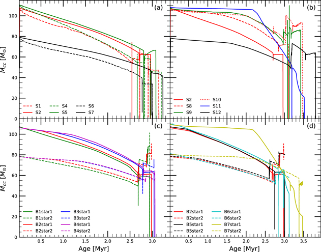
Figure 1. (a) Convective core for nonrotating single stars with different convective criteria as a function of evolutionary ages. (b) Convective core for single stars with different various metallicities and rotational velocities as a function of evolutionary ages. (c) Convective core for the donor star (solid lines) and the accreting star (dashed lines) in the binary system with differential orbital period as a function of evolutionary ages. (d) Convective core for two components in the binary system with different metallicities and stellar mass as a function of evolutionary ages.
Download figure:
Standard image High-resolution image3.1.2. Evolution of the Hydrogen Profile
Figure 2 illustrates the evolution of the hydrogen profile in a nonrotational 130 M⊙ Population III star with Schwarzschild convection and Ledoux convection criteria. It is displayed that the Ledoux convection model S1 can attain the helium core at the central hydrogen exhaustion and favor the dredge-up. When convective motion attains the hot layers that are rich in carbon and oxygen, energy generation in the H-burning shell increases dramatically and triggers the expansion of the envelope to large radii. In model S1 using the Ledoux criterion, convection shifts outward after the end of core hydrogen burning because the molecular weight gradient prevents inward movement and mixing of hydrogen into carbon-rich layers. In model S2 using the Schwarzschild criterion, convection moves inward during the core He-burning phase. However, there appears to be a significant distance between convection front and central helium cores. For instance, mass coordinates for helium cores are 67.27 M⊙, whereas they are 71.92 M⊙ for convection fronts at a central helium mass fraction of 0.9. This fact implies that the model with the Schwarzschild criterion does not easily form the deep dredge-up.
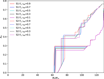
Figure 2. Evolution of the H profile in a 130 M⊙ Population III star with Schwarzschild and Ledoux convection criteria during the core He-burning phase. The legend shows evolved stages in central helium in mass fraction.
Download figure:
Standard image High-resolution image3.1.3. Evolution in H-R Diagram
Figure 3(a) displays the evolution of nonrotational single stars in the Hertzsprung–Russell (H-R) diagram. It is found that models using the Schwarzschild convection criterion can widen the main-sequence width and lengthen the main sequence because of the larger extension of the convective core. A larger amount of hydrogen is available for helium production in the core and leads to a larger helium core (panel (a1) in Figure 10). The star displays a lower effective temperature and a higher luminosity at the end of the main sequence. This implies that stars with a Schwarzschild convection criterion have larger radius.
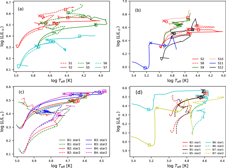
Figure 3. Panels (a)–(d) display evolutionary tracks in the H-R diagram. The lines have the same meaning as in panels (a)–(d) of Figure 1.
Download figure:
Standard image High-resolution image3.1.4. Evolution of Stellar Mass
Figure 4(a) illustrates the evolution of stellar mass for nonrotational single stars as a function of evolutionary age. As expected, the main sequence is barely affected for Population III stars in panel (a). The reason is the extremely low value of radiative winds during this phase. The mass-loss rate for 130 Population III stars with a Schwarzschild convection criterion is larger during the post–main-sequence phase compared to the one during the main sequence. The nonrotational model S2 suffers a huge amount of mass loss during the post–main-sequence because it approaches Eddington luminosity. Its surface effective temperature falls down to  (see Figure 3). The star turns back blueward in the H-R diagram owing to mass removal. If the stellar evolution timescale is long compared to the growth time of the instability, which is of order the thermal timescale of the convective element, then the temperature gradient from the Schwarzschild convection model is appropriate (Lawlor et al. 2015). In the following sequences, we use the Schwarzschild convection criterion to model the evolution of rotating single and binary Population III stars.
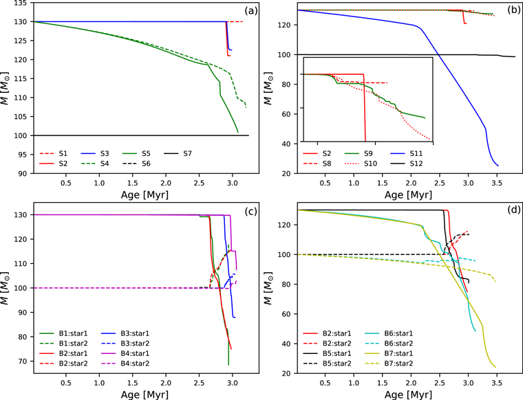
Figure 4. Panels (a)–(d) illustrate that stellar mass varies with the evolutionary age. The lines have the same meaning as in panels (a)–(d) of Figure 1.
Download figure:
Standard image High-resolution image3.2. Evolution of Rotating Single Population III Stars
3.2.1. Evolution of Rotational Velocities
Figure 5 shows the relationship between the equatorial rotational speeds and evolutionary ages for single stars and binarities. For the nonrotating model S2, the rotational velocity maintains zero until the end of the calculation. We find that rotational velocities in rotating models increase toward critical velocities, except for model S11. Actually, from the beginning of evolution, spin angular velocities go down slightly owing to the combined effect of mass loss via stellar winds and stellar expansion. Therefore, the increase of rotational velocities mainly originates from the expansion of stellar radius. The growth of the ratio of angular velocities  in panel (c) can be explained by three reasons. First, the angular velocity Ω decreases less steeply with the stellar radius than Ωcrit (∝R−3/2) for Population III stars. Second, the removal of angular momentum via stellar winds during evolution is much weaker than the counterparts with high metallicity. Third, there is some transport by shear induced by the angular velocity gradient that forms between the contracting core and the expanding envelope, instead of meridional circulations that might be negligible for Population III stars. The results indicate that the internal transport of angular momentum from the stellar interior to the surface is sufficient to bring the surface to critical rotation during the main sequence. This process effectively compensates the decreasing of angular velocities thanks to stellar expansion and wind braking. Model S11 has a higher initial value of
  than other models because the quantity
  is proportional to the quantity of R1/2. Moreover, Ωcrit decreases with the increasing of metallicity Z because the star with higher metallicity Z has a larger radius.
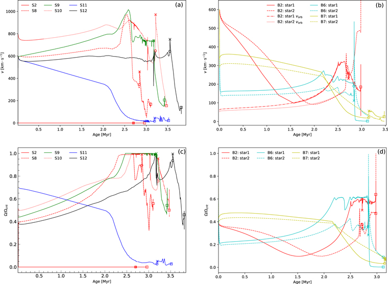
Figure 5. (a) Surface equatorial rotational velocity for single-star models as a function of evolutionary ages until the end of the calculation. (b) Surface equatorial rotational velocity for two components in binarities as a function of evolutionary ages. (c) Evolution of the ratio of angular velocities to the critical angular velocity (i.e.,  ) for single stars. (d) Evolution of
  for two components in binarities. Different evolutionary points of the star are marked with different symbols: circles—the terminal of main sequence; crosses—the beginning of the central helium burning; squares—the end of the central helium burning.
Download figure:
Standard image High-resolution imageAs shown by the comparison of model S8 with model S11, rotational velocities for model S11 with Z = 0.0021 decline rather rapidly, while they go up for model S8 at Z = 10−14. The reason is that the mass-loss rate by stellar winds is expected to depend on the chemical composition of the atmosphere as  with m = 0.85 for Vink et al. (2001). This indicates that at high metallicity Z there will be larger mass loss than at lower metallicity Z, so less angular momentum will be kept in the star with high metallicity Z at the surface. Actually, meridional circulations are much more efficient at high metallicity Z at feeding the surface with angular momentum than the ones at lower metallicity Z. This fact implies that wind mass loss, which removes mass and thus spin angular momentum, has exceeded the outward transportation of angular momentum induced by meridional circulations in model S11. It is also displayed in Figure 5(a) that model S12 with a lower stellar mass reaches the critical velocity later. There are three main reasons. First, meridional circulations and shears that can transfer angular momentum are weaker in low-mass stars than in high-mass stars. Second, the critical velocity goes up for decreasing mass, which is due to the decreasing contribution of radiation pressure. Third, the expansion of low-mass stars is slower than that of high-mass stars.
Although the initial rotational velocities for S10 are highest, they attain the critical velocities later (see Figures 5(a) and (c)). There are two main reasons. First, this physical process can be explained by the fact that Population III stars do not experience significant mass loss at the beginning of evolution because lines by hydrogen and helium are too weak to trigger radiation-driven winds (Krticka et al. 2006). However, when core temperature attains Tc ∼ 108 K, helium fusion via 3α-reaction starts to generate 12C. When the mass fraction of 12C attains the value of  , the CNO cycle is activated and the C, N, O elements are diffused from the stellar core to the surface by meridional circulations. Vink & de Koter (2005) have noticed that most of the opacity driving of the radiative winds is due to iron (70%, and 15% to CNO) at solar metallicity Z. However, CNO contributes to 60% of the driving and Fe to 10% at Z⊙/30. CNO (to some extent extended to H and He) lines govern the wind-driving mechanism instead of only H and He lines, and then this results in stronger winds that remarkably reduce rotational velocities. Second, the radius expands slowly owing to quasi-chemically homogeneous evolution (hereafter, quasi-CHE) for S10, and this process can lead to a higher critical rotation (see Figure 7).
It takes a significant fraction of evolutionary time for models S8 and S10 to maintain critical velocity because critical velocity declines with stellar expansion. Rotational velocities for S2 and S10 can attain the critical velocity again during the Hertzsprung gap. The reason is that violent expansion results in strong differential rotation, which can efficiently transfer spin angular momentum outward. Moreover, rapid contractions of the convective envelope easily bring the star to critical rotation (Heger & Langer 1998). Rotation velocities for models S8 and S10 fall with the rapid expansion of envelopes during helium burning because of the conservation of spin angular momentum. This fact also indicates that large amounts of mass may be lost at this advanced stage.
3.2.2. Evolution of Stellar Mass and Convective Cores
Figure 4(b) shows stellar mass for single stars as a function of evolutionary age. Comparing models S8 and S10, one can find that the amount of mass lost is higher for rapidly rotating stars during the main sequence. For comparison, one can notice that mass loss also increases with the increase of mass and metallicity. Because W-R stars generate a much larger amount of carbon and other elements than stars that do not go through the W-R phase, the mass-loss rate for model S11 goes up rapidly during the main sequence. A bi-stability jump can occur in model S8. The effect of mass loss can bring about lower luminosity because the luminosity is directly proportional to the power law of stellar mass (Kippenhahn & Weigert 1990).
It is shown in Figure 1(b) that the convective core for model S8 is smaller than the one for model S2 at or near ZAMS. The reason is that centrifugal forces partly sustain the star against its own gravity. Therefore, model S8 behaves like a lower-mass nonrotating one. This leads to a smaller luminosity in the H-R diagram. In fact, the size of the convective core is governed by radiative pressure. Therefore, convective cores in low-mass model S12 are smaller than those in model S8.
Away from ZAMS, convective cores appear to be larger in the star with high velocity because rotational mixing becomes efficient. The larger core induced by rotational mixing gives rise to higher central temperature and lower opacity. Meridional circulation governs rotational mixing above the convective core because the gradients of chemical elements decrease the shear turbulence (Song et al. 2018a). The core for the star with Z = 10−14 has a smaller value than the one for the star with Z = 10−8 because of the weak released luminosity. The maximum size of the convective core occurs for model S11 with CHE because rotational mixing is so efficient that hydrogen and helium diffuse freely without the restrictions of μ-gradients.
Close to the hydrogen exhaustion, the convective core for S2 has a value of  , whereas it has a value of ∼72.74 M⊙ for S8. Therefore, convective cores can be remarkably enlarged by rotational mixing. In convective regions, the density gradient is smaller; thus, more matter is contained in a given volume. This enables local gravity to be larger, and thus the star is better counteracted against the centrifugal force. This implies that rotational mixing gives rise to a larger mean density and a more compact star. Furthermore, the rotationally induced mixing refuels the core in fresh hydrogen and contributes to higher luminosity. The corresponding lifetime of main sequence is significantly prolonged. By comparing models S2 and S10, one finds that rotational mixing also delays the shrinkage of the convective core. The decreasing of the core size may occur just when the model starts to lose a huge amount of matter. When evolution proceeds, model S11 has a smaller convective core owing to mass removal via W-R winds.
3.2.3. Nitrogen and Helium Enrichments
Figure 6(a) displays surface nitrogen abundances for the single star as a function of evolutionary age. Nitrogen enrichment for S2 and S3 can be ascribed to mass removal of hydrogen envelopes via stellar winds after main sequence. Markova et al. (2018) have noticed that the envelope is really stripped in the most luminous supergiants by the strong winds ( and
and ![$\mathrm{log}\dot{M}[{M}_{\odot }\,{\mathrm{yr}}^{-1}]\geqslant -5.4$](https://content.cld.iop.org/journals/0004-637X/892/1/41/revision1/apjab7993ieqn79.gif) ). Maeder et al. (2009) pointed out that the behavior of the excess of nitrogen abundances is a multivariate function (i.e., stellar mass, evolutionary age, projected rotational velocity, metallicity) for a single rotating star. As expected, we find that nitrogen enrichment goes up with the increase of initial velocity and evolutionary age during the main sequence when comparing models S8 and S10. Moreover, nitrogen enrichment for model S9 is higher than the one for model S8. Surface nitrogen abundance reaches quite high values for model S11 with CHE because more nitrogen can be synthesized via CNO cycles in the star with high values of initial CNO. After helium burning, surface nitrogen abundances increase rapidly because W-R winds expose nitrogen at the position of hydrogen-burning shells.
). Maeder et al. (2009) pointed out that the behavior of the excess of nitrogen abundances is a multivariate function (i.e., stellar mass, evolutionary age, projected rotational velocity, metallicity) for a single rotating star. As expected, we find that nitrogen enrichment goes up with the increase of initial velocity and evolutionary age during the main sequence when comparing models S8 and S10. Moreover, nitrogen enrichment for model S9 is higher than the one for model S8. Surface nitrogen abundance reaches quite high values for model S11 with CHE because more nitrogen can be synthesized via CNO cycles in the star with high values of initial CNO. After helium burning, surface nitrogen abundances increase rapidly because W-R winds expose nitrogen at the position of hydrogen-burning shells.
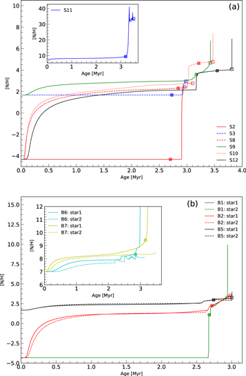
Figure 6. (a) Surface nitrogen abundances as a function of evolutionary age in single stars. (b) Surface nitrogen abundances as a function of evolutionary age for the donor star and the accreting star in binarities.
Download figure:
Standard image High-resolution imageOne can find that nitrogen enrichments in less massive stars S12 proceed slower than the ones in massive stars S8 at early stages of main sequence. However, less massive Population III stars may be responsible for the overabundance of nitrogen at the subsequent stage. There are three main reasons. First, a high rotational velocity for model S12 favors efficient carbon mixing between helium-burning cores and hydrogen-burning shells. Second, more primary nitrogen can be produced at the position of hydrogen-burning shells. Third, the surface nitrogen enrichment factor can attain a value of 1.23 during the dredge-up. These lower-mass Population III stars contribute through their winds to the enrichment in newly synthesized elements of the interstellar medium. This may be closely related to unusually high nitrogen abundances found in extremely metal-poor objects (CS 22949–037). This star was discovered to have an extreme overabundance of nitrogen relative to iron (Norris et al. 2001).
Figure 7(a) shows surface helium mass faction Ys versus central helium mass fraction Yc from ZAMS up to the end of the helium burning for single stars. Surface helium abundance for model S1 goes up at the end of helium burning because stellar winds expose the productions of the hydrogen-burning shell. Note that surface helium enrichment for model S2 appears after main sequence owing to the dredge-up. In contrast to model S11, other rotational sequences do not undergo CHE, and their surface becomes less enriched with helium. Model S10 represents a transition between CHE and normal evolution and is marked as quasi-CHE. It is difficult for Population III stars to form CHE because meridional circulations are too weak to give rise to rapid mixing. Model S11 displays the CHE, and its surface helium abundance goes up as fast as the central He abundance during the main sequence. At core hydrogen exhaustion, surface helium mass fraction has attained a value close to 1. The star can turn into a massive helium star with a very thin radiative envelope. After main sequence, surface helium abundance decreases steeply in the second half of helium burning. This can be ascribed by the fact that helium is mixed from radiative envelopes to convective cores, whereas both carbon and oxygen in the core are transferred to the envelope. Surface helium abundance for other Population III stars remains approximately the constant value because hydrogen envelopes of these stars are very thick.
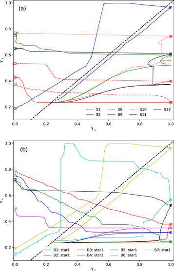
Figure 7. Surface helium mass faction Ys vs. central helium mass fraction Yc from ZAMS up to the end of the helium burning for (a) single stars and (b) the donor star in binaries. When the surface helium abundance goes up as fast as the central helium abundance (slope ∼ 1), the evolution is chemically homogeneous. For comparison, a straight line with a slope of 1 is included (black dashed line).
Download figure:
Standard image High-resolution image3.2.4. The Evolution of Surface Hydrogen and Effective Temperature
Panels (a) and (b) in Figure 8 show the evolution of the mass fraction of hydrogen and effective temperature as a function of the central helium mass fraction. From panel (a), one can find that models S2 and S8 cannot turn into W-R stars, which are defined as  and XH < 0.4 because hydrogen envelopes are not removed significantly by weak stellar winds. One can also find that surface mass fraction of hydrogen goes down rapidly with the increase of rotational velocities and metallicity. Meanwhile, the star shifts toward high temperature during the main sequence in panel (b). There are small round excursions for models S9, S10, and S12 at central hydrogen exhaustion because of the first dredge-up. Surface hydrogen drops rapidly during the first dredge-up. For instance, surface hydrogen mass fraction for S12 falls down from 0.441 to 0.254, whereas the corresponding effective temperature goes up from 4.538 to 4.817. The first dredge-up can cause the star to shift toward higher effective temperature and can favor the formation of W-R stars. Model S11 is first transformed into a W-R star because it has experienced CHE. Therefore, it will take more time for model S11 to evolve at the stage of W-R stars, and stellar mass is smaller at the end of helium burning. Model S12 turns into W-R stars later because mass loss induced by rotation is weak for lower-mass stars.
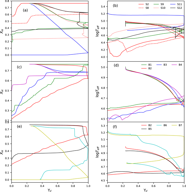
Figure 8. (a) Evolution of surface mass fraction of hydrogen as a function of the central He mass fraction for single stars. (b) Evolution of the effective temperature as a function of the central He mass fraction for single stars. (c) and (e) Evolution of surface mass fraction of hydrogen as a function of the central He mass fraction for the donor star in binarities. (d) and (f) Evolution of the effective temperature as a function of the central He mass fraction for the donor star in binarities.
Download figure:
Standard image High-resolution image3.2.5. Chemical Structure
Figure 9 shows mass fraction of various chemical elements as a function of the mass coordinate for models S2 and S8. The abundances show a step profile above the convective core at the end of hydrogen burning, representing outer convective regions. One can notice that the included masses for outer convective regions in model S2 are smaller than the ones for S8. For example, we have the following mass sizes for the two convective layers: between 86.35 and 100.33 M⊙ for model S2 (i.e., 14 M⊙), and between 102 and 123 M⊙ for model S8 (i.e., 21 M⊙). Therefore, rotation favors convection in stellar envelopes and thus leads to the deep dredge-up.
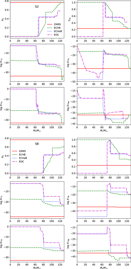
Figure 9. Mass fraction of H, He, C, N, O, and Ne as a function of the mass coordinate for the nonrotational model S2 and rotational model S8 at different evolutionary points as indicated by the different colors: ZAMS (red solid lines); the end of central hydrogen burning (marked by ECHB; green dashed lines); the end of central helium burning (marked by ECHeB; blue dashed lines); the end of calculation (marked by EOC; purple dashed–dotted lines.)
Download figure:
Standard image High-resolution imageSurface abundances for 1H in model S10 are reduced, whereas surface abundances of He, C, O, N, Ne, Mg, and 26Al are increased by rotational mixing at hydrogen exhaustion in comparison with model S2 without rotation (see Table 3). One can find that during the main sequence surface carbon and oxygen abundances decrease in S11, whereas they go up in S8. This fact implies that these chemical elements are transferred inward in S11 and are transported outward in Population III stars in S8. We have noticed that the high surface abundances of carbon, nitrogen, and oxygen for model S10 make the metallicity Z up to 1.26 × 10⁻⁷, whereas these abundances are less than 10−12 in the nonrotating model S2. This results in a stronger mass-loss rate for stellar winds. Note that helium burning via the 3α-reaction may produce C and O in the core, and carbon is transported to the envelope by rotational mixing. After that, some amounts of C and O are brought from the core to the hydrogen-burning shell, which has a much higher temperature and is closer to the core for Population III stars. These two elements are processed to not only nitrogen but also all the other CNO nuclei by CNO cycles. Rotational velocities and central temperature are higher for Population III stars, and they have created favorable conditions that can reproduce the occurrence of primary nitrogen.
Most of the CEMP-no stars (i.e., carbon-enriched extremely metal-poor stars without r- and s-process elements) display not only an enriched C abundance but also excesses in nitrogen and oxygen. Maeder & Meynet (2015) have presented that the variety of abundances found at the surface of such stars can be explained by various degrees of back-and-forth mixing between the hydrogen- and helium-burning regions. The released energy in the hydrogen shell goes up dramatically and drives the expansion of the hydrogen envelope to larger radii. Therefore, the dredge-up is easy to develop (see Figure 14(a)). The production of primary nitrogen can be greatly influenced by mass loss because H-burning shells (i.e., the engine for the production of primary nitrogen) for model S11 can be extinguished by a strong W-R wind at central helium of 0.8. In this case, CEMP-no stars might also be explained by the convective dredge-up.
One can find that the nitrogen peak for S8 at the position of the H shell increases remarkably and diffusion spreads nitrogen further outward and inward. Nitrogen in the hydrogen-burning shell that is diffused back to the center is quickly converted into 22Ne first and then into 25,26Mg, turning into an efficient primary neutron source. Then, central abundances for 14N and 22Ne are increased by this interplay (Meynet & Maeder 2002; Limongi & Chieffi 2018). More importantly, the helium that is produced in H-burning shells is also transferred towards the helium-burning core, and it supports the conversion of 12C into 16O, reducing therefore the final 12C/16O ratio in the CO core. Therefore, surface abundances of O, 20Ne, and Al go up remarkably for model S8 during central helium burning.
3.2.6. The Evolution of Helium Cores
Panels (a1)–(a4) in Figure 10 display the evolution of helium cores for single stars. We have noticed that the helium core for model S1, which has a value of 54.65 M⊙, disappears at the evolutionary time of 2.541 Myr and displays a larger one of 57.38 M⊙ again at the evolutionary time of 2.69 Myr. The reason is that the first deep dredge-up can mix the hydrogen from the envelope to the core at hydrogen exhaustion. Hydrogen burning may be reignited and can generate a larger helium core. We can notice that nonrotational models S1 and S4 with the Ledoux convection criterion have experienced two episodes of deep dredge-up, whereas models S2 and S5 with the Schwarzschild convection criterion have not gone through the deep dredge-up. During the dredge-up, both the central temperature and mean molecular weight are decreased, while the opacity is increased owing to the engulfed hydrogen. Although model S12 has experienced the dredge-up, helium cores in S8 are larger than that in S12 in panel (a2). The reason is that helium cores scale with the size of the hydrogen convective core and increase with the initial mass of the star. Radiative pressure is larger for more massive stars and results in larger helium cores.
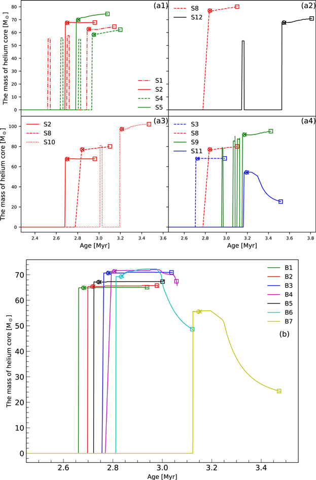
Figure 10. (a1) Evolution of the mass of helium cores for single stars with different convective criteria. (a2) Evolution of the mass of helium cores for different stellar mass. (a3) Evolution of the mass of helium cores for single stars with different initial velocities. (a4) Evolution of the mass of helium cores for different initial metallicities. (b) Evolution of the mass of helium cores for the donor star in binaries.
Download figure:
Standard image High-resolution imageFrom panel (3a), we can find that model S8 has a helium core with a mass of 77.33 M⊙ at 2.685 Myr, whereas model S2 has a helium core with a mass of 67.31 M⊙ at 2.685 Myr. Therefore, rotational mixing can remarkably increase the mass of the helium core during the main sequence. In order to obtain such mixing, large overshooting is often introduced in the literature (Chin & Stothers 1991). Both rotational mixing and larger overshooting can result in bigger CO core masses and therefore tracks in the ρc–Tc diagram that are moved toward the pair-instability region (i.e.,  ). Helium cores for S8 increase slightly because the H-burning shell continuously adds new helium mass to the He core. It is noticed that model S10 goes through the dredge-up owing to higher initial rotational velocities (see Appendix B). Maeder & Meynet (2008) have presented that the effects of rotation on the thermal gradient are much larger and that rotation triggers convection in stellar envelopes. We have noticed that the convective dredge-up might prefer the lower-mass star with higher rotational velocities and metallicities. From panel (a3), helium cores for model S9 with high metallicities are larger compared to model S8. However, helium cores for model S11 reduce substantially because of the strong stellar wind expected at the phase for W-R stars.
3.2.7. Evolution in H-R Diagram
Panel (3b) in Figure 3 shows the evolution of single stars in the H-R diagram. On or close to ZAMS, effective temperature  and luminosity
  of model S2 are 5.004 and 6.319, respectively, whereas their values in rotational model S10 are 4.972 and 6.301, respectively (see Table 2). Therefore, rapid rotation may enable the star to shift toward low temperature and luminosity. There are two main reasons. First, the centrifugal force gives rise to a weaker effective gravity, which can contribute to lower central temperature and smaller convective core. For example, at the age of ∼0.0489 Myr, the mass of the convective core of model S2 is 106.99 M⊙, whereas it is 105.71 M⊙ for model S10 (see Figure 1(b)). Second, low effective gravity can result in low surface temperature and luminosity according to gravity darkening (von Zeipel 1924). Generally, the star with low metallicity Z is more compact, and density profiles are flatter in the interior of this model owing to larger cores. Therefore, the luminosities for the star with low Z can be more influenced by rotation.
Moreover, one can find that at ZAMS the effective temperature  and luminosity
  for model S11 are 4.746 and 6.264, respectively whereas their values for model S8 are 4.995 and 6.307, respectively. This indicates that low-metallicity model S8 gives rise to lower opacities, which generate a bigger outgoing luminosity. The radiative gradient
  is smaller because of both the smaller opacity and the higher internal temperature. This leads to larger surface effective temperature for Population III stars.
Nonrotational model S2 shows a quite large span of temperature at almost constant luminosity after main sequence, which is caused by a rapid expansion of the envelope during evolution. It evolves redward to the temperature of  , implying that they become blue supergiant stars. One can find that the more rapidly rotating stars in S10 remain bluer and are more luminous than the nonrotational stars in S2. The reason is that the increase of helium in outer envelopes leads to a declining of the opacity and a growing in mean molecular weight, resulting in more luminous and more compact stars. Actually, stellar contraction and expansion in the outer envelope are governed by the photon luminosity and therefore by the opacities. The luminosity available for stellar expansion is decreased by rotational mixing because the envelope becomes transparent. Moreover, the decreased specific entropy may originate from the increasing of mean molecular weight in the outer envelope. At the same time, fresh hydrogen is mixed into the core and thus contributes to a higher specific entropy.
The central compactness, which is defined by the ratio of central density to mean density (i.e.,  ), increases with the initial rotational velocity on or close to ZAMS. Rapid rotation enables stars to turn into a central compact one. In order to offset the centrifugal force, more matter tends to deposit toward the core for increasing the local gravitational force (see Table 2). Therefore, rapid rotation is not in favor of fast apsidal motion, which has been found by Claret (1999). However, the central compactness is decreased by rotational mixing at the subsequent stage. The reason is that rotating mixing brings about a lower central density ρc, which originates from inward hydrogen mixing in the core and a higher mean density
  due to a smaller radius. For instance, model S2 inflates to a value of
  at hydrogen exhaustion, whereas model S10 expands to a radius of
  (see Table 2).
The model S11 can undergo CHE because the chemical mixing timescale induced by Eddington–Sweet circulations can be shorter than the nuclear burning time of hydrogen. Model S11 shifts toward blueward instead of redward on the H-R diagram. The reason is that effective temperature for a homogeneous star has a power law of 1.5 with mean molecular weight (i.e., Teff ∝ μ1.5M0.75). Because almost all the hydrogen in the star takes part in nuclear reaction in this way, the star gradually turns into a massive helium star on main sequence. The central temperature and specific entropy are lower for model S11 in contrast to Population III stars. Except for the surface layer, there appears to be a flat entropy profile inside the star with CHE. The luminosity for model S11 with CHE falls down rapidly at the stage for W-R stars because the decreasing of stellar mass exceeds the increasing of mean molecular weight (i.e.,  ). CHE is an important evolutionary channel that can generate massive He stars at low metallicities, but it is difficult for Population III stars to produce CHE. For a given mass, meridional circulations for Population III stars proceed much slower than the ones in stars with high metallicity because weak angular momentum loss via stellar winds restricts the velocity of meridional circulations. The rotational mixing timescale will be longer than the nuclear timescale. Model S10 goes through a quasi-CHE, and its effective temperature lies between CHE and normal evolution.
3.3. The Evolution of Binary Population III Stars
3.3.1. Evolution of Rotational Velocities
Figures 5(b) and (d) illustrate that rotational velocities and corresponding angular velocities of the primary star (more massive star; solid lines) and the secondary star (less massive star; dashed lines) vary with evolutionary age. It is shown that equatorial velocities of both components in binaries drop from ZAMS as a result of tidal interactions. The reason is that tidal torques can spin the star down when the spin angular velocity is larger than the orbital one. The primary star for models B2, B6, and B7 attains a synchronous state (i.e., Ω1 = Ωorb) at an age of 1.607, 0.0181, and 0.00215 Myr, respectively. The secondary star in B2 achieves this state at 1.944 Myr. The fact indicates that synchronous timescales become larger for less massive components with low metallicity owing to a smaller radius. The main reason is that synchronous timescales are sensitive to the factor  according to Zahn (1977). The quantity R is stellar radius, and the value a is the orbital separation. Furthermore, tidal torques are proportional to the factor of E2 (i.e.,
  ), which is smaller for less massive stars. Population III stars can maintain higher rotational speeds in a longer evolutionary time than the counterparts with high metallicity, and rapid rotation for Population III stars can slow down the production of mean molecular weight gradients, which can efficiently inhibit rotational mixing in the stellar interior.
As expected, the synchronous timescale also has a bigger value in the system with a longer orbital period. Rotational velocities for two components in model B4 behave as the ones for single stars owing to a larger initial orbital period. Therefore, a single star can maintain a high rotational velocity, whereas rotational velocities are braked by tidal torques in the binary system, except for the system with a very large orbital period.
At the synchronous state, tidal torque is zero according to Equation (20) in Paxton et al. (2015). Both components can be spun down further by stellar winds. Spin velocities of two components finally attain the equilibrium velocity, which is always slightly inferior to the orbital one (Song et al. 2018a, 2018b). For example, at the evolutionary age of 1.793 Myr, the equilibrium velocity for the donor star in model B2 is 112.18 km s−1, whereas the orbital velocity is 115.85 km s−1. We have derived a theoretical equation for the equilibrium velocity in Appendix A. For the donor star in model B2, we obtain the quantities τmc = 0.493 Myr, τmi = 2.703 Myr, τwb = 220.32 Myr, and τtide = 0.0150 Myr, respectively. The theoretical value for equilibrium velocities is 111.82 km s−1, which is very close to the numerical solution of 112.18 km s−1. The fact indicates that the equilibrium velocity strongly depends on the timescales of stellar expansion, tidal torques, wind torques, and meridional circulations. Tides tend to spin surface layers of the star up, whereas other mechanisms (i.e., meridional circulations, wind braking, and stellar expansion) are inclined to spin the star down at the equilibrium state.
After synchronization, equatorial velocities of both components in models B2 and B6 increase owing to stellar expansion because spin angular velocities are locked to approach the orbital one. The donor star in models B2 and B6 suffers from heavy mass and angular momentum loss during the first episode of RLOF. This process can efficiently spin the donor star down. Mass and angular momentum are transferred to the companion star. Generally, the spin-up torque due to RLOF is 3–4 orders of magnitude larger than tidal torques (Song et al. 2017). Packet (1981) has found that only about 10% of the stellar material is able to spin the companion star up significantly. The accreting star attains critical rotation once for models B2 and B6 during RLOF.
The accreting star for B7 is not spun up to critical velocities because of the deficiency of RLOF, in comparison with binary Population III stars. W-R winds for model B7 take away the specific orbital angular momentum of the mass-losing star and broaden the orbital separation evidently. Rotational velocities of two components go down progressively because two components undergo CHE.
3.3.2. The Evolution of Orbital Periods and Mass Transfer Rates due to RLOF
Figure 11 shows the evolution of the orbital period for the binaries. One may find that the orbital period for B2 is slightly larger than the one for B1 before RLOF. The reason is that tidal torques spin the star down when the spin angular velocity of two components is larger than the orbital one. More spin angular momenta can be converted into the orbit, and thus the orbital period is increased. Therefore, model B1 starts RLOF at the time of 2.640 Myr, whereas model B2 starts RLOF at the time of 2.518 Myr. The orbital period for models B3 and B4 remains unchanged during the main sequence because the tidal torques are very weak owing to the larger initial orbital period. This implies that there is no or very tiny angular momentum exchange between spin angular momentum and the orbital one. Furthermore, stellar winds for models B3 and B4, which can widen the orbital separation, are also very negligible.
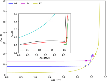
Figure 11. Evolution of the orbital period for binaries.
Download figure:
Standard image High-resolution imageThe orbital period for B6 increases faster than the one for B5 before RLOF. There are two main reasons. First, during synchronization (i.e., before the age of 0.0286 Myr), the efficiency of exchange of angular momentum is much higher. Second, stellar winds for model B6 are much stronger. The orbital period for all binaries goes up continuously before mass reverse because the accretion efficiency is so low that the inefficient mass transfer can not cause the orbit to shrink (Song et al. 2018b). Also, critical rotation for the accreting star induced by RLOF can enlarge the orbital period rapidly because most transferred matter is thrown away from the system in a form of winds. For instance, the orbital period for B2 increases from 4.16 to 11.48 days, whereas it increases from 4.00 to 9.73 days for the B1 system. The mass transfer phase generally terminates when the donor star has been stripped of most of its envelope. The hydrogen-burning shell can be extinguished, and the corresponding engine that produces primary nitrogen is turned off. For instance, hydrogen-burning shells for the donor star in B6 and B7 extinguish at central helium Yc = 0.639 and 0.818, respectively. However, the donor star still has some hydrogen left in its envelope (typically a few 0.1 M⊙). Strong mass loss via W-R winds in model B7 tends to widen the orbit dramatically in comparison with model B4.
Figure 12 displays the mass transfer rate due to RLOF as a function of evolutionary age in binaries. It is found in panel (a) that the peak of mass transfer rate during the first episode of RLOF increases with the orbital period because the donor star evolves fully. The mass transfer rate in Model B4 can reach 3.7 × 10⁻³ M⊙ yr−1 because the donor star has developed a convective envelope. Although the orbit for high-metallicity model B6 is enlarged by strong stellar winds, it begins mass transfer early at the time of 2.186 Myr. The reason is that the radius for model B6 is much larger than the one for model B2. During the first episode of RLOF, the peak of the mass transfer rate is high for Population III stars. For example, the mass transfer rate for B2 is 9.98 × 10⁻⁴ M⊙ yr−1, whereas it has the value of 1.684 × 10⁻⁴ M⊙ yr−1 in B6. The reason is that less mass is lost by stellar winds in B2 and more mass can be transferred to the companion star correspondingly. Wider systems induced by strong stellar winds also do not favor RLOF because their Roche lobe is larger (see Table 4). For example, at the beginning of RLOF, the orbital period for B2 is 4.16 days, whereas it can arrive at a value of 6.26 days for B6. During the two episodes of RLOF, the donor star loses 54.65 M⊙ for B2, whereas it loses 17.19 M⊙ for B6.
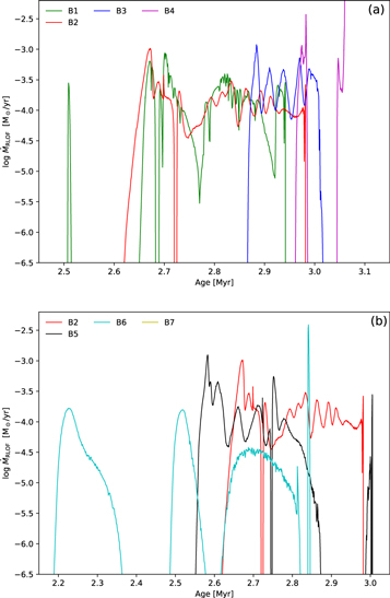
Figure 12. Evolution of mass transferring rate due to RLOF in binaries.
Download figure:
Standard image High-resolution image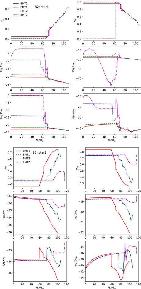
Figure 13. Mass fraction of H, He, C, N, O, and Ne as a function of the mass coordinate for the donor star (star 1) and the accreting star (star 2) in rotational binary model B2. Different evolutionary stages are indicated by the different colors: the beginning of the first episode of RLOF (red solid lines), the terminal of the first episode of RLOF (green dashed lines), the beginning of the second episode of RLOF (blue dotted lines), and the terminal of the second episode of RLOF (purple dashed–dotted lines.)
Download figure:
Standard image High-resolution image3.3.3. The Evolution of Convective Cores
Panels (c) and (d) of Figure 1 show the evolution of the convective core mass for the binaries. It is clear that the convective core for model B6 shrinks faster than the one for model S11 from ZAMS because rotational velocities can be braked by tidal interactions during synchronization. This implies that rotational mixing effectively mixes the hydrogen from the envelope to the core and slows down the reduction speed of Thomson scattering opacity (i.e., κTh = 0.2(1 + XH)), which originates from the consumed core hydrogen. Like model S11, the donor star for model B7, which has gone through CHE, has the largest convective core during the main sequence. The convective core for the donor star in B7 does not undergo rapid contraction at core hydrogen exhaustion because of CHE.
Matter is transferred to the companion star owing to RLOF. The donor star responds to the removal in mass by decreasing its convective cores. The accreting star responds to the increase in mass by increasing convective cores. The size of its convective core goes up, and fresh hydrogen is mixed toward the center, effectively rejuvenating the star. After accretion, the properties of the star resemble the properties of a younger single star of the same mass. The accreting star becomes brighter but remains hot, appearing as an O-type star (see panel (c) of Figure 3). An exception appears in the donor star in B4, and convective cores do not decrease owing to mass removal. This implies that the donor star with central helium burning does not respond to the decreasing in convective core mass rapidly by adapting its internal structure. It is found that in wider systems convective cores for two components can grow larger before RLOF starts. The reason is that tidal braking is too weak to reduce rotational mixing. The shorter the initial orbital period, the smaller the mass of convective cores for the donor star after mass transfer. This can be understood by the fact that more mass can be transferred to the companion star in the system with shorter orbital period (see Figure 4(c)). One can find that the accreting star with higher metallicity can obtain less mass, except for model B7, which goes through CHE.
3.3.4. Nitrogen and Helium Enrichments in Binaries
Figure 6(b) illustrates that surface nitrogen abundances of two components in binaries vary with evolutionary age. Nitrogen enrichment for the donor star in B1 occurs (i.e., t = 2.66 Myr) early in comparison with the one in model S2 (i.e., t = 2.90 Myr) because RLOF can quickly expose the inner hydrogen-burning region, which is rich in nitrogen. Nitrogen enrichment for the nonrotating accreting star in B1 can also reach a high value as a result of the transferred matter. Nitrogen abundances for model S8 reach 2.11 dex at 2.0 Myr, whereas it arrives at 1.34 dex for model B2 owing to tidal braking. The result indicates that nitrogen enrichment is weaker in binarities than the one in single stars. A very interesting case occurs in model B5. Nitrogen enrichment for the less massive accreting star can outweigh the more massive donor star during synchronization. The reason is that the accreting star can maintain a higher rotational speed owing to a longer timescale for synchronization (see Figure 5(b)). It is difficult for two components in binarities to produce CHE unless the orbital period is extremely short (de Mink et al. 2009; Song et al. 2016). After synchronization, rotational velocities can attain high values in an extremely tight binary system, which are beneficial to mixing chemical elements (see Figure 7(b)). This case may happen in model B7. These facts indicate that rotational mixing in binaries does not heavily depend on the initial rotational velocity but is strongly related to the orbital period.
In contrast with rotational models for single stars, nitrogen enrichment in binaries does not depend on stellar mass. The low-mass components may show the high surface nitrogen abundance because of the mass reverse during RLOF. There is only a mild or no nitrogen enrichment for the accreting star in rotational sequences during RLOF in comparison with nonrotational sequence B1. There are three main reasons (Song et al. 2018b). First, mass gainers stop accretion when its outer layers rotate critically. The transferred matter, which is rich in nitrogen, will deposit in an outer disk surrounding the accreting star. This matter might be dissipated by high radiative pressures. Second, thermohaline mixing swiftly dilutes the accreted nitrogen within the thermal timescale, which is very short for massive stars. We can notice that four peaks for model B6 in Figure 6(b) indicate that mass transfer due to RLOF occurs at these episodes. The decline of nitrogen after peaks implies that the thermohaline instability allows mixing downward of the accreted nitrogen-rich matter to occur. Third, the accretor has been spun down by tidal torques during previous synchronization, and this process easily develops a high gradient of mean molecular weight at the boundary of the convective core, which can drastically slow down rotational mixing. The transferred matter that is enriched in CNO elements produces strong stellar winds for the accreting star because the reduced opacity in the outer envelope also contributes to high temperature and luminosity.
Figure 7(b) displays surface helium mass faction Ys versus central helium mass fraction Yc from ZAMS up to the end of the helium burning for the donor star in binaries. Surface helium abundance for B6 reaches a value of ∼0.566 at the terminal of the main sequence, while it has a value of ∼0.97 for S4. Therefore, CHE can be inhibited in binarities except for the system B7 with very short orbital period (de Mink et al. 2009). At the end of central helium burning, surface helium mass fraction from model B1 to model B4 can reach the values of 0.715, 0.787, 0.757, and 0.500, respectively. The result indicates that rotation can expose more helium and less helium enrichment happens in wider systems. At the same time, the surface helium mass fraction for models B5 and B6 can reach values of 0.719 and 0.1497, respectively. Therefore, the system with high metallicities appears to have a lower surface helium mass fraction. System B7 does not experience RLOF at all, and no mass transfer occurs in this system. Surface helium abundance for the donor star in models B6 and B7 progressively increases after the main sequence because of the combined effect of RLOF and W-R winds. Then, it falls down rapidly because of the removal of helium envelopes and the exposure of CO cores. After the main sequence, the surface helium abundance for the donor star in systems B1–B5 increases gradually with the exposing of the products for hydrogen-burning shells.
3.3.5. The Evolution of Surface Hydrogen and Effective Temperature in Binaries
Panels (c)–(d) of Figure 8 illustrate the evolution of mass fraction of hydrogen and effective temperature as a function of the central helium mass fraction in binaries. Before RLOF, the surface hydrogen fraction decreases slowly for model B2 because mass loss induced by rotation is decreased by tidal braking in comparison with the one for B4. Furthermore, the surface hydrogen fraction for model B7 is lower in comparison with B2 because stars with high metallicity have strong winds. Rapid decreasing of hydrogen in B7 can cause the star to shift toward high effective temperature, whereas model B2 evolves toward low effective temperature. Surface hydrogen fraction falls down steeply for close binaries because hydrogen envelopes are removed remarkably by RLOF. Therefore, there is no dredge-up that occurs in binaries. There is also some indication that the total hydrogen content may be a function of the initial orbital period. Larger orbital periods give rise to a larger hydrogen content. The surface hydrogen fraction disappears early for model B7 with CHE. The surface hydrogen mass fraction for B2 vanishes earlier than the counterpart for B3 because the donor star for model B2 turns into W-R stars early. One can find that high-metallicity stars B6 display a higher effective temperature at the terminal of helium burning because of the removal of a huge amount of hydrogen envelopes.
3.3.6. Chemical Structure
Figure 13 illustrates the mass fraction of H, He, C, N, O, and Ne as a function of the mass coordinate for two components in model B2. After the second episode of RLOF, surface abundances for H decline while surface abundances for He, C, N, O, and 22Ne increase for two components in B2. This indicates that chemical elements in the envelope for the donor star can be transferred to the accreting stars owing to RLOF. Moreover, convective cores for the donor star are reduced, whereas convective cores for the accreting star are increased correspondingly. The central abundance of H increases for the accreting star, whereas central He, C, N, O, and Ne decline owing to the expansion of convective cores. This implies that the chemical structure of the accreting star can be significantly modified by RLOF.
Before RLOF, one can find that surface abundances for H, 22Ne, and Mg go down sightly while surface abundances for He, C, N, O, and Al go up owing to rotational mixing, by comparing the donor star in B1 with the one in B2 (see Table 5). Surface abundances for He, C, N, O, 20Ne, and Al go up in B2, while surface abundances for H, 22Ne, and Mg go down sightly owing to RLOF. At hydrogen exhaustion, surface Mg abundance for the donor star in model B3 increases remarkably, and less Al is enriched in contrast to B2. The reason is that RLOF does not occur in model B3 during the main sequence and a higher temperature might remain inside the star (see Table 4). During helium burning, surface abundances for H, He, N, and Al go down remarkably while surface abundances for C, O, Ne, and 25Mg go up in models B6 and B7. This can be ascribed to the fact that hydrogen envelopes have been removed for the star with high metallicities. Stellar mass for the donor star in B1 has a value of 79.37 M⊙, whereas it is 75.09 M⊙ for the one in B2 at the end of the second episode of RLOF. Therefore, rotation tends to produce stellar expansion and greatly favors RLOF in the binary system. At the end of central helium burning, surface abundances for He, C, and 22Ne go up for B7 with CHE, while surface abundances for N, O, 20Ne, Mg, and 26Al go down sightly compared to B6. The main reason is that the donor star in model B7 with CHE has a minimum value of mass (see Table 5).
3.3.7. The Evolution of Helium Cores
Panel (b) of Figure 10 displays the evolution of helium cores for the donor star in the binarities. The mass of helium cores for rotating stars in close binaries will often be smaller than the counterpart in single stars or wide binaries. For example, helium cores for S8 have a value of 76.89 M⊙ at 2.836 Myr, whereas they have a value of 65.42 M⊙ for B2 at 2.701 Myr. The reason is that helium cores are decreased by RLOF. A donor star that loses its hydrogen envelope will generate a smaller helium core compared to a single star. Furthermore, tidal braking can reduce rotational velocities and thus smaller helium cores. The donor star from model B1 to model B4 has values of 64.91, 65.42, 70.58, and 71.28 M⊙, respectively. The results reveal that the shorter the initial orbital period, the smaller the mass of helium cores. This fact implies that more matter can be transferred toward the companion star in a system with shorter orbital period. Moreover, helium cores for models B5 and B6 have values of 67.31 and 69.38 M⊙, respectively. This can be understood by the fact that the orbital separation can be widened via strong winds in the system with high metallicities and contribute to larger Roche lobe. Mass transfer rates due to RLOF are lower in system B6. We can notice that there is no deep dredge-up for binaries compared to single stars because of RLOF. However, helium core mass is 55.60 M⊙ for model B7 with CHE, and it is the smallest one. This is expected because the star has turned into a W-R star during the main sequence. Strong W-R winds can reduce remarkably the mass of helium core.
3.3.8. The Evolution in H-R Diagram
Panels (c) and (d) of Figure 3 display the evolution of two components in the H-R diagram. At the terminal of helium burning, the temperature and luminosity for model S2 are 4.389 and 6.565, respectively, whereas they are 4.596 and 6.526 for model B1 (see Tables 2 and 4). The effective temperature is increased, whereas the luminosity is decreased in binarities because the hydrogen envelopes are stripped owing to RLOF. However, the temperature and luminosity for model B2 are 4.581 and 6.543, respectively. Rotation can cause the star to shift toward lower temperature and high luminosity because less mass is transferred to the companion star. The donor star in model B6 makes a small blue loop at hydrogen exhaustion, and they turn into W-R stars later in contrast to the one in model B7. The evolution of the donor star in B7 has the same trend as model S11 because both of them go through CHE.
The secondary star in B1 is able to accrete the matter coming from the donor star efficiently, and then it may contract appreciably, attaining high effective temperature. Podsiadlowski et al. (1992) have presented that an important factor in determining the time of transition to the low temperature is the fractional core mass  , where mc is the mass of the hydrogen-exhausted core and M is the total mass of the star. Therefore, accretion of matter from a close binary tends to increase the mc, which can cause the star to prevent the transition to the red supergiant stage. The accreting star in B4 shifts toward low effective temperature because it merely obtains the least matter from the donor star (see Figure 4(c)). From Figure 3(d), one can also notice that the accreting star in B6 shifts toward low effective temperature, whereas the one in B5 evolves toward high effective temperature. The main reason is that the high-metallicity star B6 loses a large amount of mass via stellar winds, and thus less matter can be transferred toward the companion star.
4. Summary and Discussion
Models using the Schwarzschild convection criterion can widen the main-sequence width and lengthen the main sequence because of the larger extension of the convective core. A larger amount of hydrogen is available for helium production in the core and leads to a larger helium core. The star displays a lower effective temperature and a higher luminosity at the end of the main sequence. Nonrotational models using Ledoux convection models can attain the helium core at the central hydrogen exhaustion and form the dredge-up.
Massive nonrotational stars of Population III may lose mass in helium-burning phases when they attain the Eddington limit, experiencing a period of very high mass loss that triggers the ejection of a substantial fraction of the H-rich envelope. The strong mixing produced by rotation brings some CNO elements at the stellar surface, which thus increases the metallicity and allows the radiative stellar winds to be active in Population III.
The increase of rotational velocities for Population III stars can be attributed to the increase of the radius. Population III stars spend a substantial amount of time on critical rotation with the radius increasing. Rotational velocities for the star with high metallicity decrease rapidly because these stars lose a major fraction of their hydrogen-rich envelope via strong winds. During synchronization, two components in binarities can be braked by tidal interactions. However, Population III stars can maintain higher rotational velocities because their radii are smaller. The donor star in binarities has suffered from both heavy mass and spin angular momentum loss owing to RLOF, and it can be spun down further after synchronization. The transferred matter can spin the accreting star up to critical rotation because the accreting star obtains a considerable amount of mass and angular momentum.
The theoretical equilibrium velocity has been derived from various timescales (i.e., the timescales for meridional circulations, tidal interactions, wind braking, and the expanding radius), and it is always slightly inferior to the synchronous one. Tidal torques that tend to spin the star up counteract with other mechanisms, which incline to spin the star down. The equilibrium velocity approaches the synchronous velocity with the orbital shrinkage.
Rotation reduces convective cores at ZAMS because the centrifugal force enables the star to behave like a lower mass star. However, rotational mixing can enlarge convective cores because meridional circulations mix the fresh hydrogen-rich matter inward from the envelope to the core. The decreasing of the core mass occurs just when the model starts to lose a large amount of mass via stellar winds. The convective core for the binarities shrinks faster than the one for single stars during synchronization because rotational velocities have been braked by tidal interactions.
After helium burning, surface nitrogen abundance for W-R stars increases rapidly because stellar winds expose nitrogen at the position of hydrogen-burning shells. The first dredge-up can mix chemical elements in the star and bring some fraction of fresh hydrogen from the envelope to the helium core. This process can significantly reduce central temperature and density and thus enlarge the main-sequence lifetime for Population III stars. Helium, carbon, nitrogen, oxygen, and neon are mixing up into the envelope, and a significant amount of nitrogen and neon is produced inside the star. The opacity can be increased by the first dredge-up. We have noticed that a single 100 M⊙ Population III star may exhibit high nitrogen enrichment compared to single 130 M⊙ Population III stars after main sequence. This scenario indicates that nitrogen enrichment may be possible to explain with relatively low mass stars.
Less mass is lost by stellar wind, and much matter can be transferred to the companion star. The peak of the mass transfer rate is high for Population III stars. Wider systems induced by strong stellar winds also do not favor RLOF because their Roche lobe is large. Also, critical rotation for the accreting star induced by mass transfer can enlarge the orbital period because most transferred matter is thrown away from the system in the form of winds. There appears to be no RLOF in models with CHE because the radii for two components inflate very slowly or even shrink during the main sequence.
Stellar contraction and expansion in the outer envelope are governed by the photon luminosity and therefore by the opacities. The increase of helium in the envelopes due to rotational mixing leads to a decrease of the opacity and an increase in mean molecular weight. The luminosity available for stellar expansion is decreased by rotational mixing. The decreased specific entropy may result from a change of mean molecular weight. At the same time, fresh hydrogen is mixed into the core, and thus rotational mixing contributes to a higher specific entropy. Furthermore, the central compactness is reduced whereas the central temperature is increased by rotational mixing.
The first dredge-up can increase the mass of helium cores and thus the central temperature. The convective dredge-up might prefer the lower-mass star with higher rotational velocities and metallicities. It can also help to produce W-R stars because a huge amount of hydrogen in the envelope is mixed into the core. The mass of helium cores for stars in binaries with the short orbital period will often be smaller than the one in single stars or wide binaries. Convective cores for the donor star are reduced, while convective cores for the accreting star are increased owing to RLOF. The mass of helium cores for massive stars is larger than the one for less massive stars because radiative pressure is larger for more massive stars. Moreover, helium cores for W-R stars fall down rapidly because mass loss via W-R winds is strong enough to reduce helium cores substantially.
Surface abundances for hydrogen in single rotating Population III stars are reduced, whereas surface abundances for He, C, N, O, and Al are increased at hydrogen exhaustion. Helium burning via 3α-reaction may produce C in the core, and carbon is transported to the envelope. Some amounts of C and O are brought from the core to the hydrogen-burning shell. These two elements are processed to produce nitrogen and other CNO nuclei. The nitrogen peak at the position of the H shell is diffused back to the center and is quickly converted into 22Ne first and then into 25,26Mg, turning into an efficient primary neutron source. Then, central abundances for 14N and 22Ne are increased by this interplay. The hydrogen-burning shell becomes more active, which powers the expansion of the hydrogen envelope to large radii.
After the second episode of RLOF, surface abundances for H decline while surface abundances for He, C, N, O, and 22Ne increase for two components in B2. This indicates that chemical elements in the envelope for the donor star can be transferred to the accreting stars owing to RLOF. Central abundances of H, C, N, and O increase for the accreting star, whereas central He and Ne decline owing to convective cores expanding, which is induced by RLOF. For the star with high metallicity, the hydrogen-burning shell vanishes rather soon because of the removal of hydrogen envelopes via W-R stellar winds.
Chemically homogeneous stars evolve blueward during the main sequence. They have the largest convective core, and the corresponding envelope is absent owing to efficient rotational mixing. They display a flat entropy profile inside the star and turn into W-R stars early. Surface helium abundance for these stars goes up as fast as the central helium abundance. Strong W-R winds enable the star to shrink greatly, and the star attains a smaller mass. Therefore, they display a lower luminosity and a higher effective temperature after the main sequence. They also possess remarkable surface C, O, and 22Ne enrichment and corresponding surface H, He, N, and Al deficiency at helium exhaustion. There is no obvious difference for surface chemical elements between single stars with CHE and binary stars with CHE.
In this paper, we mainly focus on the evolution of both hydrogen- and helium-burning phases. Actually, rotation is still important in causing additional mixing during the advanced burning stages, especially by shear instabilities (Heger et al. 2000). There is also a cumulative effect because the larger helium cores obtained from calculations that include rotation affect the nucleosynthesis and structure through all phases (Heger & Woosley 2002; Woosley 2002). With regard to angular momentum, rotation becomes an important dynamic effect during core collapse (Heger et al. 2000; Maeder & Meynet 2001) since all current gamma-ray-burst models that invoke massive star progenitors require considerably higher angular momenta (Woosley & Heger 2012; Woosley 2017). The detailed evolutionary single and binary models at the late stages are indicated to explore these underlying physical processes, and these problems are beyond the scope of this paper. We will investigate these important issues in our next work.
This work was sponsored by the National Natural Science Foundation of China (grant Nos. 11863003, 11463002), the Swiss National Science Foundation (project No. 200020-172505), and the Science and Technology Planning Project in Guizhou Province (grant No. [2018]5781). We are very grateful to an anonymous referee for his/her valuable suggestions and very insightful remarks, which have improved this paper greatly. We also thank Dr. Sylvia Ekström for her very kind help and discussion.
Appendix A: The Theoretical Equation for Equilibrium Velocities
The variation of spin angular momentum for the primary star can be given by

where I1 is the moment of inertia of the primary star,  is the change of the spin angular momentum due to tidal interaction and is given by (Zahn 1977)

and
where M, R, Ω1, and τtide, respectively, are the total mass, radius, and spin angular velocity of the primary star; the timescale for tides, τtide, is defined as  ; ωorb is the orbital angular velocity; a is the separation between the two components of the binary system (we assume a circular orbit); and E2 is the tidal coefficient that can be expressed by
  (Hurley et al. 2002) and
  . The quantity
  is stellar wind braking, and it can be expressed as

where  is the mass-loss rate of stellar wind and is a negative value.
At the equilibrium state, tidal torques counteract with wind braking, meridional circulation, and the variation of moment of inertia. From Equation (1), we obtain

that is,
where τwb is the timescale of wind braking and is defined as  (Song et al. 2018a). We have used the relationship (
 +
+  +
+  ).
).  is the velocity of meridional circulations, which are the main factor that transfers the angular momentum inside the star.
In order to find the equilibrium angular velocity ωequil, we put  in the above equation. At the equilibrium state, meridional circulations tend to transfer the angular momentum from the surface to the interior and spin the star down. We make use of the relationship
  because the gradient of angular velocity is positive (Song et al. 2013). Finally, we can obtain

where τmi is the timescale of the variation of moment of inertia and is defined as  . According to the equation for angular momentum transport, τmc is given by
  . Finally, the equilibrium spin angular velocity is given by

Form the above equation, we can obtain the equilibrium velocity ( ). The timescale for tides τtide is much shorter than other timescales (i.e.,
 ![${\tau }_{\mathrm{tide}}\ll \mathrm{Min}[{\tau }_{\mathrm{wb}},{\tau }_{\mathrm{mc}},{\tau }_{\mathrm{mi}}]$](https://content.cld.iop.org/journals/0004-637X/892/1/41/revision1/apjab7993ieqn112.gif) ); for the equilibrium tide, the equilibrium angular velocity approaches the orbital one. For a single rotating star, we derive an important equation from Equation (6),
); for the equilibrium tide, the equilibrium angular velocity approaches the orbital one. For a single rotating star, we derive an important equation from Equation (6),

Mass transfer due to RLOF can spin the donor star down and can also spin the accreting star down from the equilibrium velocity. We can add a term  , which stands for the torque due to RLOF on the right of Equation (6), and derive an equation for the donor star
where suffix 1 denotes the donor star. The equation for the accreting star is
Appendix B: The First Dredge-up in the Model S10
The top panel of Figure 14 shows a zoom-in from the Kippenhahn diagram for model S10 during the first dredge-up. The dredge-up occurs when surface effective temperature Teff becomes low enough that the base of the surface convection region shifts inward to where it meets the convection zone above the H-burning shell. The hydrogen-burning shell is very close to the helium cores. Occasionally, external convective envelopes move inward and attain the helium core, which is produced by hydrogen burning, and thus this process contributes to the deep dredge-up. The convective envelope penetrates deeply into the hydrogen-exhausted core in S10 and dredges up a significant fraction of CNO production.
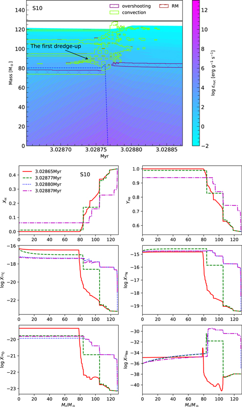
Figure 14. Top panel: Kippenhahn diagram for model S10. Green hatched regions are convective, and purple hatched regions are overshooting. Pink shaded regions indicate the energy generation for hydrogen burning. Bottom panel: variation of profiles for various chemical elements with evolutionary age in model S10.
Download figure:
Standard image High-resolution image
The bottom panel of Figure 14 illustrates the evolution of profiles of various chemical elements during the first dredge-up. The inner layers that have gone through helium burning are both C-rich and O-rich. When convective cells attain these regions, helium, carbon, nitrogen, oxygen, and neon are mixing up into the envelope. At the same time, fresh hydrogen flows into the central core. Note that the star is rejuvenated by the dredge-up. The temperature in the core is high enough to reignite CNO cycles and can generate hydrogen burning. It can be very efficient because of the high carbon mass fraction and therefore gives rise to a significant amount of nitrogen and neon in the core. This process can significantly reduce central temperature and mean molecular weight and thus enlarge the main-sequence lifetime. The opacity can be increased by the dredge-up. Therefore, model S9 shifts back and forth in the H-R diagram (see Figure 3(b)). As a result of the dredge-up, the nitrogen enrichment factor for model S10 reaches 1.76, whereas it can attain 1.23 for S12. Nitrogen enrichment during the dredge-up is small for these two models because the duration is very short (see Table 3).