


Abstract
We theoretically verify that optical vortices carrying orbital angular momentum are generated in various astrophysical situations via nonlinear inverse Thomson scattering. Arbitrary angle collisions between relativistic electrons and circularly polarized strong electromagnetic waves are treated. We reveal that the higher harmonic components of scattered photons carry well-defined orbital angular momentum under a specific condition that the Lorentz factor of the electron is much larger than the field strength parameter of the electromagnetic wave. Our study indicates that optical vortices in a wide frequency range from radio waves to gamma-rays are naturally generated in environments where high-energy electrons interact with circularly polarized strong electromagnetic waves at various interaction angles. Optical vortices should be a new multi-messenger member carrying information concerning the physical circumstances of their sources, e.g., the magnetic and radiation fields. Moreover, their interactions with matter via their orbital angular momenta may play an important role in the evolution of matter in the universe.
Export citation and abstract BibTeX RIS

Original content from this work may be used under the terms of the Creative Commons Attribution 3.0 licence. Any further distribution of this work must maintain attribution to the author(s) and the title of the work, journal citation and DOI.
1. Introduction
Unlike a plane wave, an electromagnetic wave with the spiral phase term,  , possesses a helical wavefront and varies its phase in the transverse plane, where n is an integer and ϕ is the azimuthal angle around the central axis of propagation. Such an electromagnetic wave is called an optical vortex. Optical vortex photons carry discrete values
  of orbital angular momentum (OAM) around their propagation axis in addition to spin angular momentum (SAM), where ℏ is the Planck constant divided by 2π (Allen et al. 1992, 1999). The transverse intensity distribution shows an annular shape associated with a phase singularity at the central axis.
Studies on optical vortices are currently spread over the micro (Tamburini et al. 2011a, 2012; Olivier et al. 2016), terahertz (Imai et al. 2014), visible (Yao & Padgett 2011; Taira & Zhang 2017), ultraviolet (Terhalle et al. 2011; Bahrdt et al. 2013; Katoh et al. 2017b; Rebernik Ribic et al. 2017), keV X-ray (Peele et al. 2002; Sasaki & McNulty 2008; Kohmura et al. 2009; Takahashi et al. 2013; Vila-Comamala et al. 2014), and MeV and GeV gamma-ray (Jentschura & Serbo 2011; Liu et al. 2016; Taira et al. 2017) frequency ranges. Vortex beams have also been generated in a sub-MeV electron (Uchida & Tonomura 2010; Verbeeck et al. 2010; McMorran et al. 2011; Béché et al. 2014) and a cold neutron (Clark et al. 2015; Sarenac et al. 2016). Interactions between optical vortices carrying OAM and matter have been investigated. The transfer of OAM has been experimentally demonstrated in particle manipulations (Simpson et al. 1997; O'Neil et al. 2002) and photoexcitation (Schmiegelow et al. 2016; Peshkov et al. 2017; Afanasev et al. 2018a). Theoretically, optical vortices in the ultraviolet, X-ray, and gamma-ray frequency range likely trigger new phenomena in photoionization (Picón et al. 2010), a dichroic effect (van Veenendaal & McNulty 2007), and Thomson and Compton scattering (Stock et al. 2015; Maruyama et al. 2017; Sherwin 2017), photodisintegration (Afanasev et al. 2018b), and photonuclear reactions (Taira et al. 2017).
Possible roles of optical vortices in astrophysics have been discussed (Harwit 2003; Elias 2008), and it has been argued that normal photons are converted into vortex photons in several astrophysical environments such as around Kerr black holes (Tamburini et al. 2011b) and in nonuniform plasma (Tamburini et al. 2010; Gray et al. 2014). Several methods to observe optical vortices from astronomical objects have been proposed (Berkhout & Beijersbergen 2008; Uribe-Patarroyo et al. 2011). However, radiation processes capable of creating optical vortices in astrophysical situations have rarely been discussed until recently.
Inverse Thomson and Compton scattering, which produce high-energy photons in the X-ray and gamma-ray frequency ranges, are important radiation processes in astrophysics. Here, we distinguish inverse Thomson scattering as being a scattering process where the energy of the scattered photon is much smaller than the initial electron energy. Inverse Thomson and Compton scattering occurs when a relativistic electron interacts with a low-energy photon (an electromagnetic wave). The strength of the electromagnetic wave is characterized by a dimensionless field strength parameter,

Here, e is the elementary charge, me is the electron rest mass, c is the speed of light, ω0 is the angular frequency of the initial electromagnetic wave, and A0, E0, and B0 are the maximum amplitudes of the initial vector potential, electric field, and magnetic field, respectively. When an electron interacts with a strong electromagnetic wave of  , the nonlinear effect of inverse Thomson and Compton scattering becomes prominent and higher harmonic photons are emitted in addition to the fundamental radiation (Esarey et al. 1993). Nonlinear inverse Thomson and Compton scattering has been theoretically investigated for sources of intense X-rays and gamma-rays using relativistic electron beams and high-power lasers (Esarey et al. 1993; Ride et al. 1995; Hartemann et al. 2000; Dongguo et al. 2003; Krafft & Priebe 2010; Sakai et al. 2011) and has actually been observed in laboratories (Bula et al. 1996; Burke et al. 1997; Babzien et al. 2006; Sakai et al. 2015). In astrophysics, this process has been discussed as a candidate for radiation processes, e.g., in pulsars (Gunn & Ostriker 1971; Arons 1972; Stewart 1972).
In our previous work, we revealed that a gamma-ray vortex can be generated by a head-on collision between a high-energy electron and an intense circularly polarized laser via nonlinear inverse Thomson scattering (NITS). We showed that the nth harmonic gamma-rays produced in this process have the spiral phase term  and carry OAM equal to
  (Taira et al. 2017). The annular intensity distribution of the second harmonic X-rays calculated by the derived equations reproduced a previous experimental result (Sakai et al. 2015). This implies that optical vortices are generated in environments where high-energy electrons interact with circularly polarized strong electromagnetic waves. Such environments may be commonplace in the universe, such as in the vicinity of magnetized near neutron stars and in turbulent plasma in astrophysical jets. However, under such astrophysical situations, electrons should interact with electromagnetic waves not only head-on but also at arbitrary angles. In this paper, we treat NITS in a more relevant manner for astrophysics by expanding our previous work to include arbitrary angle interactions. We demonstrate that optical vortices are generated when the Lorentz factor of the initial electron is much larger than the field strength parameter of the initial electromagnetic wave. To our knowledge, this is the first theoretical study showing that optical vortices are naturally created by NITS in astrophysical situations.
The contents of this paper are as follows. In Section 2, we derive theoretical equations for electron motions inside a circularly polarized strong electromagnetic wave and for the electric field of the scattered photon. In Section 3, we describe how higher harmonic photons have an annular intensity distribution, spiral phase term, and carry OAM. We show several numerical examples of the number of scattered photons and their energy. In Section 4, we discuss several possible astrophysical situations where optical vortices may be emitted by NITS.
2. Theoretical Treatment of NITS at Arbitrary Angle Interactions
2.1. Motion of an Electron Inside a Circularly Polarized Strong Electromagnetic Wave
The motion of an electron inside a circularly polarized electromagnetic wave has been treated using classical electrodynamics in several previous studies (Gunn & Ostriker 1971; Stewart 1972; Ride et al. 1995). In this paper, we follow the notation described in Ride et al. (1995). The coordinate systems used in the calculation are shown in Figure 1. Here, we assume that the circularly polarized strong electromagnetic wave is propagating in the -z direction. The normalized vector potential of the circularly polarized electromagnetic wave is expressed as

Here,  and λ0 are the wave number and the wavelength of the initial electromagnetic wave, respectively,
  is an independent variable, t is time, and
  and
and  are the unit vectors along the x- and y-axes, respectively.
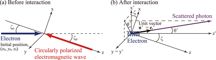
Figure 1. Coordinate systems used in the calculation. Before the interaction, the initial electromagnetic wave moves toward the initial electron at the incident angle, ζ0. After the interaction, the mean velocity of the electron is directed along the z'-axis, which is inclined to the z-axis by an angle ζ. A photon is scattered in a direction with an angle θ' with respect to the z'-axis and an angle ϕ' with respect to the x'-axis.
Download figure:
Standard image High-resolution imageThe electron is initially moving in the x–z plane at an angle ζ0 with respect to the z-axis with a normalized velocity  , where
  is the initial electron velocity,
  ,
,  (Figure 1(a)), and
  is a unit vector along the z-axis. The electron momentum normalized by the electron rest energy during the electron and electromagnetic wave interaction is written as
  , where γ and
  are the Lorentz factor and the normalized velocity of the electron, respectively. The vector components of
  in the coordinate system
  can be expressed as follows by solving the relativistic Lorentz equations:


Here,  . The averages of the components over the electromagnetic wave period are given by the following:


Even though the average electron momenta along the x- and y-axes conserve the initial momenta, the momentum along the z-axis is reduced by  . The decrease in the average electron momentum is due to the ponderomotive force of a strong electromagnetic wave (Ride et al. 1995). Consequently, the propagation direction of an electron within a strong electromagnetic wave is slightly changed from the initial direction. We define the electron as moving along the z'-axis within the electromagnetic wave (Figure 1(b)). The angle between the z- and z'-axes is given by
  , where
  . Note that the photon is scattered into a narrow cone centered about the z'-axis. Therefore, to see the phase structure of the scattered photon, we should consider the electron trajectory in the coordinate system
  .
.
First, we consider the electron orbits,  , inside the circularly polarized electromagnetic wave in the coordinate system
  . These orbits are derived using the relation
  and are given by the following:


Here, x0, y0, and z0 are the initial positions of the electron along the x-, y-, and z-axes, respectively, r1 is the radius of the electron motion given by

and  and
and  are given by

Therefore,  .
.
The unit vectors in the two coordinate systems  and
and  are transformed by the following relations:


Therefore, the electron orbits,  , in the coordinate system
  are given by

In general, Equations (18)–(20) do not represent a helical circular motion. We can rewrite Equations (18)–(20) by introducing a quantity  , which is much smaller than unity under the conditions of
  and
and  . The coefficients of
  in Equations (18) and (20) can then be expressed as


Here, we used the relation
To derive Equations (21)–(23), we assumed the following condition:
Therefore, Equations (18)–(20) can be rewritten as

When  , Equations (25)–(27) indicate that the electron motion is well represented by a helical circular trajectory in the coordinate system
  , in which the electron moves counterclockwise when the observer is facing the oncoming electron. We call this electron motion positive helicity.
2.2. The Electric Field of the Scattered Photon
The Fourier component of the electric field emitted by a single electron can be calculated from the Lienard–Wiechert potentials (Section 14.5 in (Jackson 1999)):
where  and ω are the wave number and the angular frequency of the emitted photon, respectively,
  is the permittivity of a vacuum, R is the distance from the origin to the observation point,
  is a unit vector pointing from the origin to the observation point as shown in Figure 1(b), and
  is the electron orbit described in Equations (9)–(11). Equation (28) can be calculated in the spherical coordinate system
  with unit vectors
  using the following relation:

where
Each component of the electric field in the spherical coordinate system is expressed as follows:
Here,  ·
· and
and  , where N0 is the number of periods of the initial electromagnetic wave interacting with the single electron. The variable
  will change according to the initial interaction angle. In a head-on collision (ζ0 = 0 rad),
  corresponds to half the longitudinal pulse width of the initial electromagnetic wave. In a 90° collision (ζ0 = π/2 rad),
  corresponds to the transverse radius of the initial electromagnetic wave if the longitudinal pulse width is longer than the transverse diameter and it corresponds to the half the longitudinal pulse width of the initial electromagnetic wave if the transverse diameter is longer than the longitudinal pulse width (Ride et al. 1995).
The unit vectors  are given by

The phase term in Equations (31) and (32) can be written in the form

where

The inner products in Equations (31) and (32) are expressed as
Finally, Equations (31) and (32) can be written in the limit  as follows:
Here, n is an integer and Jn and  are the Bessel function of the first kind and its derivative, respectively. The details of the derivation of Equations (43) and (44) are described in the Appendix. Equations (43) and (44) peak at a wave number given by

This equation indicates that n is the harmonic number of the scattered photon, as described in Equation (58).
To show the phase structure in the transverse plane against the z'-axis, we express the electric field in the Cartesian coordinate system  , as shown below:


Therefore, the electric field is
Here, the electric field is expressed by the complex orthogonal unit vectors  whose helicities of the circularly polarized electric fields are positive and negative, respectively. For the positive helicity, the rotation of the electric field is counterclockwise when the observer is facing the oncoming radiation that is denoted as right-hand circular polarization (Hamaker & Bregman 1996; Trippe 2014). Conversely, for the negative helicity, the rotation of the electric field is clockwise and the radiation is denoted as left-hand circular polarization.
In the paraxial approximation (θ' ≪ 1), the longitudinal component of the electric field along the z'-axis is much smaller than the transverse component. With the assumption of  and R ∼ z1 (z1 is the distance along the z'-axis from the origin to the observation point), the electric field can be expressed as follows:
2.3. Degree of Circular Polarization of the Emitted Photons
The degree of circular polarization of the emitted photon can be represented by the Stokes parameter, which is expressed as ((Hamaker & Bregman 1996; Trippe 2014), Section 7.2 in (Jackson 1999))
The Bessel function of the first kind can be expressed as (Section 2.11 in (Watson 1962))

where
When  , the Bessel function of the first kind and its derivative can be expressed as


By substituting Equations (54) and (55) into Equation (51), Equation (51) will become, in the limit of θ' ≪ 1,

where
Therefore, when  , the Stokes parameter only depends on the Lorentz factor of the initial electron, the scattering angle of the photon, and the field strength parameter of the initial electromagnetic wave. The Stokes parameter does not depend on the wavelength of the initial electromagnetic wave, the harmonic number of the scattered photon, or the initial interaction angle.
2.4. Energy of the Emitted Photons
The energy of the nth harmonic scattered photon can be calculated from Equation (45). In the limit θ' ≪ 1, the energy will be expressed as
2.5. The Transverse Energy Distribution and the Number of Emitted Photons
The radiation energy per unit angular frequency, ω, and the solid angle, Ω', is expressed as (Section 14.5 in (Jackson 1999))
Here,  . This spatial radiation energy distribution is independent of the wavelength of the initial electromagnetic wave because the variables
  ,
,  , b1, and
  are independent of the wavelength.
The number of nth harmonic photons emitted per second toward the scattering angle between  and
and  can be approximately calculated from Equation (59):
Here, F is the emission rate,
and Ne is the number of electrons interacting with the electromagnetic wave per second. Here, we made the calculation by approximating  and the bandwidth of the scattered photons arising from the finite number of periods of the initial electromagnetic wave interacting with the electron,
  (Esarey et al. 1993). The number of photons and the emission rate are proportional to N0.
3. Numerical Calculations
3.1. Polarization State and OAM
Equation (50) indicates that the electric field of the emitted photon is elliptically polarized and can be decomposed into circularly polarized components with positive and negative helicities. Each component carries  SAM and
  SAM, respectively. The positive helicity component possesses the phase term
  , which means that the fundamental component is not an optical vortex but that the higher harmonics (
 ) are vortices carrying OAM equal to
  . Conversely, the negative helicity component possesses the phase term
  and all harmonics are vortices carrying OAM equal to
  .
.
The degree of circular polarization of the emitted photon is expressed by the Stokes parameter. In the regions of  and
and  , μ of Equation (53) is less than unity up to n = 3. Therefore, the Stokes parameter is a function of the Lorentz factor, the scattering angle of the photon, and the field strength parameter. The spatial distributions of the Stokes parameter calculated from Equation (56) are shown in Figures 2(a)–(d). We used the parameters
  and a0 = 0.1–10. Stokes parameters of
  and −1 indicate 100% circular polarization with positive and negative helicity, respectively. The maximum scattering angle giving a circular polarization higher than 90% with positive helicity increases as the field strength parameter increases, as shown in Figure 2(e). Around the z'-axis in the scattering angles of
  and
and  , the degree of circular polarization is higher than 90% with positive helicity when a0 = 1 and 10, respectively. Note that the nth higher harmonic photons emitted inside this scattering angle carry OAM equal to
  . The degree of circular polarization decreases as the scattering angle increases. The polarization changes from circular polarization with positive helicity to linear polarization and then back again to circular polarization with negative helicity at large scattering angles. All harmonic photons emitted in the area of circular polarization with negative helicity carry OAM equal to
  .
.

Figure 2. The (a), (c) spatial, and (b), (d) line distributions of the Stokes parameter (V/I) of circularly polarized photons emitted by NITS. The Stokes parameter is calculated from Equation (56). The Lorentz factor of the initial electron is γ0 = 2000. The field strength parameter for panels (a) and (b) is a0 = 1, and that for panels (c) and (d) is a0 = 10. (e) Maximum scattering angle giving more than 90% of circular polarization with positive helicity as a function of the field strength parameter.
Download figure:
Standard image High-resolution image3.2. Spatial Radiation Energy Distribution
The spatial radiation energy distributions of the emitted photons for each harmonic number are shown in Figures 3 and 4. We used the parameters  , n = 1, 2, and 3, and a0 = 1 and 10 for Figures 3 and 4, respectively, and calculated the 90° interaction (ζ0 = π/2 rad). A single peaked intensity distribution is observed only for the fundamental harmonic photons (Figures 3(a) and 4(a)). An annular shape with zero intensity at the center axis can be seen only for the higher harmonics (Figures 3(b), (c), 4(b), and (c)). Note that this feature in the higher harmonics corresponds to a typical characteristic of an optical vortex. The majority of the emitted radiation energy is concentrated around the central axis where the helicity is positive. As already described, the contour of the spatial radiation energy distribution does not depend on the wavelength of the initial electromagnetic wave.

Figure 3. Spatial radiation energy distribution of the (a) first, (b) second, and (c) third harmonic photons emitted by NITS for the 90° interaction calculated from Equation (59). Each spatial distribution is normalized by the maximum value of the first harmonic. (d) Line intensity distribution along the x'-axis for each harmonic number. The lines indicate the following: long dashed line, n = 1; short dashed line, n = 2; and solid line, n = 3. The calculation parameters are γ0 = 2000, a0 = 1.0, and ζ0 = π/2 rad.
Download figure:
Standard image High-resolution image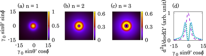
Figure 4. Same as Figure 3, but for a field strength parameter of a0 = 10.
Download figure:
Standard image High-resolution image3.3. Emission Rate of NITS Photons
Figure 5 shows the emission rate of NITS calculated from Equation (61). The emission rate is calculated by integrating the solid angle up to  , where circular polarization with positive helicity is obtained, as shown in Figure 2(e). We used the parameters
  , a0 = 0.1–10, ζ0 = π/2 rad, and N0 = 100. Here, we assume that the transverse diameter of the initial electromagnetic wave is equal to or longer than the longitudinal pulse width and
  corresponds to half the longitudinal pulse width. The emission rate as a function of the harmonic numbers and the field strength parameters are shown in Figures 5(a) and (b), respectively. The emission rate of higher harmonic photons becomes close to that of the fundamental photons as the field strength parameter increases. One can see a saturation of the emission rate in the range of
  . Therefore, the emission rates for both the fundamental and the second harmonics do not significantly change in this range. In addition, the emission rate is independent of the Lorentz factor of the initial electron, as shown in Figure 5(c). This is because the emission rate is integrated over the angle normalized by the Lorentz factor.
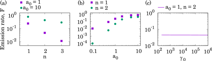
Figure 5. (a) Emission rate of NITS photons for each harmonic number calculated from Equation (61). The field strength parameter a0 is indicated in the panel. Other calculation parameters are as follows: γ0 = 2000, ζ0 = π/2 rad, and N0 = 100. (b) Emission rate of the first (n = 1) and second (n = 2) harmonic photons as a function of the field strength parameter. (c) Emission rate of the second harmonic photons vs. the Lorentz factor of the initial electron.
Download figure:
Standard image High-resolution image3.4. Energy of the Emitted Photons
As seen in Equation (58), maximum photon energy can be obtained at the center axis ( ). Figure 6(a) shows the maximum photon energy of the second harmonics as a function of the initial injection angle. The photon energy is normalized by
  . The calculation parameters can be seen in the figure. Here, we assume
  . The photon energy at the 90° interaction is half that of the head-on interaction, similar to normal inverse Thomson scattering (Taira et al. 2011). This feature of inverse Thomson scattering will enable us to produce energy tunable X-ray and gamma-ray vortices in the laboratory.

Figure 6. (a) Maximum energy of the second harmonic photon (θ' = 0) as a function of the initial injection angle calculated from Equation (58). The photon energy is normalized by  . The field strength parameter is a0 = 1. (b) Energy of the second harmonic photon with a head-on collision as a function of its scattering angle. The field strength parameters are as follows: a0 = 0.1 (dashed line) and a0 = 1.0 (solid line). (c) Maximum energy of the second harmonic photon (θ' = 0) with a head-on collision as a function of the field strength parameter.
Download figure:
Standard image High-resolution image
The energy of a photon decreases as its scattering angle increases, as shown in Figure 6(b). In addition, the energy drastically decreases in the range of  , as shown in Figure 6(c). This is due to a decrease in the longitudinal electron velocity and the growth of the transverse helical motion, as indicated in Equations (25) and (26). The photon energy is almost constant and equal to that of normal inverse Thomson scattering in the range of
  . In addition, as shown in 5(b), the emission rate of the second harmonic photons is significantly smaller than that of the fundamental photons. Therefore, when
  , the scattering process can be considered as ordinary inverse Thomson scattering.
4. Discussion
We pointed out that the helical circular motion of an electron is essential to produce optical vortices in (Katoh et al. 2017a). A photon emitted from such an electron possesses the spiral phase term and carries OAM. Helical circular motion of an electron can be achieved in laboratories using a periodic magnetic field distributed along the electron motion (Kincaid 1977) and NITS of a head-on interaction (Taira et al. 2017). In NITS at arbitrary angle interactions, however, the electron does not generally obey perfect helical circular motion. In the present study, we demonstrated that the electron obeys an approximately helical circular trajectory when the Lorentz factor of the initial electron is much larger than the field strength parameter of the initial electromagnetic wave. Under this condition, the electric field emitted from the electron possesses the spiral phase term.
We can imagine various situations in which intense electromagnetic waves and high-energy electrons coexist. Magnetic dipole radiation is thought to be emitted from pulsars when the magnetic and rotation axes are not aligned (Pacini 1968). If this is the case, in the vicinity of a pulsar, there exist extremely strong electromagnetic waves with  s−1 reaching
  (Gunn & Ostriker 1971). Because the amplitude decreases with distance from a pulsar, electromagnetic waves with
  may exist in the extended region around a pulsar. Electrons may be accelerated up to ultra-relativistic energies by various mechanisms (Ruderman & Sutherland 1975). If we assume that an electron with
  interacts with a circularly polarized strong monochromatic electromagnetic wave with
  s−1 (λ0 = 1.9 × 109 cm), a0 = 1, and N0 = 100 in the 90° direction (ζ0 = π/2 rad), second harmonic photons with a frequency
  GHz are generated at an emission rate of ∼5 × 10⁻². This radio wave vortex carries OAM equal to
  . Note that a radio wave vortex near 1 GHz carrying OAM has been generated and measured in laboratories (Tamburini et al. 2011a, 2012; Olivier et al. 2016).
Another candidate of strong electromagnetic waves is coherent synchrotron radiation, which is produced as a result of a nonuniform particle distribution (Michel 1978; Ahmadi & Gangadhara 2002) and has been discussed as a possible mechanism to produce strong radio waves (Goldreich & Keeley 1971). If we assume that an electron with γ0 = 2000 interacts with the circularly polarized radio wave with λ0 = 100 cm, a0 = 1, and N0 = 100 in the 90° direction, the wavelength of the second harmonic photons is 10−5 cm. This extreme ultraviolet vortex carries OAM equal to  . As described in Section 1, extreme ultraviolet vortices carrying OAM are thought to induce a new selection role in photoionization (Picón et al. 2010).
Relativistic shocks are thought to play an important role in various astrophysical objects such as pulsar wind nebulae, active galactic nuclei, and gamma-ray bursts (Lyubarsky 2006). Intense low frequency electromagnetic waves may be emitted by synchrotron maser instabilities at shock fronts (Hoshino et al. 1992). NITS of long wavelength electromagnetic waves may partially contribute to gamma-ray burst emissions (Preece et al. 1998; Lyubarsky 2006). The polarization of long wavelength radiation may originally be circular polarization or may have been converted from linear to circular polarization via Faraday conversion (Batebi et al. 2016). If we assume that an electron with γ0 = 1000 interacts with a circularly polarized strong monochromatic electromagnetic wave with λ0 = 3 × 10⁻³ cm, a0 = 1, and N0 = 100 in the 90° direction, the maximum energy and the emission rate of the scattered second harmonic X-rays are  and ∼5 × 10⁻², respectively. If the electron interacts with an electromagnetic wave in the head-on direction (ζ0 = 0),
  . These X-ray vortices carry OAM equal to
  .
.
Recently, circular polarization of the afterglow of a gamma-ray burst was observed at visible wavelengths; such polarization cannot be satisfactorily explained by current models (Wiersema et al. 2014). Afterglow polarization directly probes the magnetic properties of a jet. Similarly, if X-rays with OAM are observed, they will play an important role in probing the magnetic properties, as well as the circularly polarized radiation field, at gamma-ray bursts. As described in Section 1, X-rays and gamma-rays carrying OAM are thought to trigger new phenomena in a dichroic effect (van Veenendaal & McNulty 2007), Thomson and Compton scattering (Stock et al. 2015; Maruyama et al. 2017; Sherwin 2017), and photonuclear reactions (Taira et al. 2017). These new phenomena may play an important role in the evolution of matter in the universe.
Thomson scattering, which is used in this paper, is valid when the energy of the scattered photon is much smaller than the initial electron energy, i.e.,  , as described in (Esarey et al. 1993), where mec2 is the electron rest energy. When ζ0 = 0, n = 2, and θ' = 0, this relation is written using Equation (58):
When λ0 = 3 × 10⁻³ cm and a0 = 1, Equation (62) indicates  and
and  TeV. The upper limit of the Lorentz factor increases when the wavelength of the initial electromagnetic wave becomes long. Therefore, our theoretical calculation is applicable for the typical parameter regime of electrons and electromagnetic waves in pulsars and gamma-ray bursts.
This work was supported by JSPS Overseas Research Fellowships.
Appendix: Derivation of the Electric field of a Photon Emitted by NITS
The integrals of Equations (31) and (32) substituted by Equations (41) and (42) are expressed as follows:
Here, m is an integer and we used the following formulas:
Here, p is an integer. The product of the Bessel functions in Equations (63)–(66) can be simplified using Graf's addition theorem (Section 11.3 in Watson 1962):
Here,  . This formula is valid when
  . Therefore, the integral terms of Equations (31) and (32) can be expressed as

The scattered photon is concentrated around the angle  by the relativistic effect of the electron. The variables b1, b2, and Δ are approximately on the order of θ', θ'2, and θ'2, respectively. Therefore, Equations (70) and (71) can be simplified by assuming
  and
and  :
:
Finally, Equations (31) and (32) can be written as Equations (43) and (44) using the recurrence formulas,  and
and  .
.