Upper Limits on Gravitational Waves from Scorpius X-1 from a Model-based Cross-correlation Search in Advanced LIGO Data

Rotating neutron stars (NSs) are the primary expected source of continuous, periodic gravitational waves (GWs) for ground-based GW detectors. Targets include known pulsars (Aasi et al. 2014a), non-pulsating NSs in supernova remnants (Wette et al. 2008; Abadie et al. 2010; Aasi et al. 2015a), and unknown isolated (Aasi et al. 2016; Abbott et al. 2016a) or binary NSs (Aasi et al. 2014b). A particularly promising source is an accreting NS in a low-mass X-ray binary (LMXB); accretion torque spins up the NS into the frequency band of the detectors, and the accretion can generate an asymmetric mass or current quadrupole that acts as the source for the GWs (Watts et al. 2008). An approximate equilibrium between the accretion spin-up and GW spin-down, as well as other spin-down torques can produce a signal that is nearly periodic in the NS's rest frame, and then Doppler-shifted due to the orbital motion of the NS and the motion of the detector on the surface of the Earth. Such an equilibrium scenario would produce a relation between the observed accretion-induced X-ray flux of the LMXB and the expected strength of the GWs. Scorpius X-1 (Sco X-1), the most luminous LMXB, is therefore a promising potential source of GWs (Papaloizou & Pringle 1978; Wagoner 1984; Bildsten 1998). Sco X-1 is presumed to consist of an NS of mass $\approx 1.4\,{M}_{\odot }$ in a binary orbit with a companion star of mass $\approx 0.4\,{M}_{\odot }$ (Steeghs & Casares 2002). Some of the parameters inferred from observations of the system are summarized in Table 1.

Table 1.  Observed Parameters of the LMXB Sco X-1

Parameter	Value
R.A.a	${16}^{{\rm{h}}}{19}^{{\rm{m}}}55\buildrel{\rm{s}}\over{.} 0850$
Decl.a	$-15^\circ 38^{\prime} 24\buildrel{\prime\prime}\over{.} 9$
Distance (kpc)	2.8 ± 0.3
Orbital inclination ib	$44^\circ \pm 6^\circ$
K1 (km s−1)c	$[10,90]$ or [40, 90]
${T}_{\mathrm{asc}}$ (GPS s)d	$897753994\pm 100$
${P}_{\mathrm{orb}}$ (s)d	$68023.70\pm 0.04$

Notes. Uncertainties are $1\sigma$ unless otherwise stated. There are uncertainties (relevant to the present search) in the projected velocity amplitude K₁ of the NS, the orbital period ${P}_{\mathrm{orb}}$, and the time ${T}_{\mathrm{asc}}$ at which the neutron star crosses the ascending node (moving away from the observer), measured in the solar system barycenter. The orbital eccentricity of Sco X-1 is believed to be small (Steeghs & Casares 2002; Wang 2017) and is ignored in this search. The inclusion of eccentric orbits would add two search parameters that are determined by the eccentricity and the argument of periapse (Messenger 2011; Leaci & Prix 2015).

^aThe sky position (as quoted in Abbott et al. 2007a and derived from Bradshaw et al. 1999) is determined to the microarcsecond, and therefore can be treated as known in the present search. ^bThe inclination i of the orbit to the line of sight, from the observation of radio jets in Fomalont et al. (2001), is not necessarily the same as the inclination angle ι of the neutron star's spin axis, which determines the degree of polarization of the GW in Equation (1). ^cThe value of the projected orbital velocity K₁ is difficult to determine experimentally, and previous works used a value from Abbott et al. (2007a), which was derived with some assumptions from Steeghs & Casares (2002) and equivalent to $40\pm 5\,\mathrm{km}\,{{\rm{s}}}^{-1}$. The broader range listed here comes from Doppler tomography measurements and Monte Carlo simulations in Wang (2017), which show K₁ to be weakly determined beyond the constraint that $40\,\mathrm{km}\,{{\rm{s}}}^{-1}\lesssim {K}_{1}\lesssim 90\,\mathrm{km}\,{{\rm{s}}}^{-1}$. Preliminary results from Wang (2017) included the weaker constraint $10\,\mathrm{km}\,{{\rm{s}}}^{-1}\lesssim {K}_{1}\lesssim 90\,\mathrm{km}\,{{\rm{s}}}^{-1}$, which was used to determine the parameter range in Table 2. ^dThe time of ascension ${T}_{\mathrm{asc}}$, at which the neutron star crosses the ascending node (moving away from the observer), measured in the solar system barycenter, is derived from the time of inferior conjunction of the companion given in Galloway et al. (2014) by subtracting ${P}_{\mathrm{orb}}/4$. It corresponds to a time of 2008 June 17 16:06:20 UTC and can be propagated to other epochs by adding an integer multiple of ${P}_{\mathrm{orb}}$, which results in increased uncertainty in ${T}_{\mathrm{asc}}$ and correlations between ${P}_{\mathrm{orb}}$ and ${T}_{\mathrm{asc}};$ see Figure 1.

References. Bradshaw et al. (1999), Fomalont et al. (2001), Galloway et al. (2014), Wang (2017).

Download table as:  ASCIITypeset image

Several methods were used to search for Sco X-1 in data from the Initial LIGO science runs of 2002–2011: Abbott et al. (2007a) performed a fully coherent search (Jaranowski et al. 1998) on six hours of data from the second science run. Starting with the fourth science run, results for Sco X-1 were reported (Abbott et al. 2007b; Abadie et al. 2011) as part of a search for stochastic signals from isolated sky positions (Ballmer 2006). In the fifth science run, a search (Aasi et al. 2015b) was done for Doppler-modulated sidebands associated with the binary orbit (Messenger & Woan 2007; Sammut et al. 2014). In the sixth science run, Sco X-1 was included in a search (Aasi et al. 2014b) principally designed for unknown binary systems (Goetz & Riles 2011), and this method was subsequently improved to search directly for Sco X-1 (Meadors et al. 2016) and applied to Initial LIGO data (Meadors et al. 2017). A mock data challenge (Messenger et al. 2015) was conducted to compare several of the methods to search for Sco X-1, and the most sensitive (detecting all 50 simulated signals in the challenge, and 49 out of the 50 "training" signals) was the cross-correlation (CrossCorr) method (Dhurandhar et al. 2008; Whelan et al. 2015) used in the present analysis.¹⁵³

The Advanced LIGO detectors (Aasi et al. 2015c) carried out their first observing run (O1) from 2015 September 12 to 2016 January 19 (Abbott et al. 2016b). Searches for transient signals were carried out in near-real time and resulted in the observation of the binary black hole (BBH) mergers GW 150914 (Abbott et al. 2016c) and GW 151226 (Abbott et al. 2016d), and the possible BBH merger LVT 151012 (Abbott et al. 2016b), as well as upper limits on the rates and strengths of other sources (Abbott et al. 2016e, 2017a, 2017b). Searches for persistent stochastic or periodic sources were conducted using data from the full duration of the run and include searches for isotropic and anisotropic stochastic signals (Abbott et al. 2017c, 2017d) and a variety of known and unknown NSs (Abbott et al. 2017e). So far, two analyses including searches for GWs from Sco X-1 besides the current one have been released: Abbott et al. (2017d) included the direction of Sco X-1 in their directed unmodeled search for persistent GWs, and Abbott et al. (2017f) performed a directed search for Sco X-1 using a hidden Markov model.

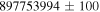
The modeled GW signal from a rotating NS consists of a "plus" polarization component, ${h}_{+}(t)={A}_{+}\,\cos [{\rm{\Phi }}(t)],$ and a "cross" polarization component, ${h}_{\times }(t)={A}_{\times }\sin [{\rm{\Phi }}(t)]$. The signal recorded in a particular detector will be a linear combination of ${h}_{+}$ and h_× determined by the detector's orientation as a function of time. The two polarization amplitudes are

$$\begin{eqnarray}&&{A}_{+}={h}_{0}\displaystyle \frac{1+{\cos }^{2}\iota }{2}\qquad \mathrm{and}\qquad {A}_{\times }={h}_{0}\,\cos \,\iota ,\end{eqnarray} \tag{ 1 }$$

where h₀ is an intrinsic amplitude related to the NS's ellipticity, moment of inertia, spin frequency, and distance; and ι is the inclination of the NS's spin to the line of sight. (For an NS in a binary, this may or may not be related to the inclination i of the binary orbit.) If $\iota =0^\circ$ or 180°, ${A}_{\times }=\pm {A}_{+}$, and gravitational radiation is circularly polarized. If $\iota =90^\circ$, ${A}_{\times }=0$, it is linearly polarized. The general case, elliptical polarization, has $0\lt | {A}_{\times }| \lt {A}_{+}$. Many search methods are sensitive to the combination

$$\begin{eqnarray}&&{({h}_{0}^{\mathrm{eff}})}^{2}=\displaystyle \frac{{A}_{+}^{2}+{A}_{\times }^{2}}{2}={h}_{0}^{2}\,\displaystyle \frac{{[(1+{\cos }^{2}\iota )/2]}^{2}+{[\cos \iota ]}^{2}}{2},\end{eqnarray} \tag{ 2 }$$

which is equal to ${h}_{0}^{2}$ for circular polarization and ${h}_{0}^{2}/8$ for linear polarization (Messenger et al. 2015; note that this differs by a factor of 2.5 from the definition of ${({h}_{0}^{\mathrm{eff}})}^{2}$ in Whelan et al. 2015).

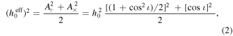
It has been suggested (Papaloizou & Pringle 1978; Wagoner 1984; Bildsten 1998) that an LMXB may be in an equilibrium state where the spin-up due to accretion is due to the spin-down due to GWs. In that case, the GW amplitude can be related to the accretion rate, as inferred from the X-ray flux F_X (Watts et al. 2008):

$$\begin{eqnarray}{h}_{0} & \approx & 3\times {10}^{-27}\,{\left(\displaystyle \frac{{F}_{{\rm{X}}}}{{10}^{-8}\mathrm{erg}{\mathrm{cm}}^{-2}{{\rm{s}}}^{-1}}\right)}^{1/2}{\left(\displaystyle \frac{{\nu }_{s}}{300\mathrm{Hz}}\right)}^{-1/2}\\ & & \,\times {\left(\displaystyle \frac{R}{10\mathrm{km}}\right)}^{3/4}{\left(\displaystyle \frac{M}{1.4{M}_{\odot }}\right)}^{-1/4}.\end{eqnarray} \tag{ 3 }$$

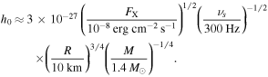
For Sco X-1, using the observed X-ray flux ${F}_{{\rm{X}}}=3.9\,\times {10}^{-7}\,\mathrm{erg}\,{\mathrm{cm}}^{-2}\,{{\rm{s}}}^{-1}$ from Watts et al. (2008), and assuming that the GW frequency f₀ is twice the spin frequency ${\nu }_{s}$ (as would be the case for GWs generated by triaxiality in the NS), the torque balance value is

$$\begin{eqnarray}&&{h}_{0}\approx 3.4\,\times \,{10}^{-26}{\left(\displaystyle \frac{{f}_{0}}{600\mathrm{Hz}}\right)}^{-1/2}.\end{eqnarray} \tag{ 4 }$$

Recent works (Haskell et al. 2015a, 2015b) have cast doubt on the ubiquity of the GW torque balance scenario in light of other spin-down mechanisms; the torque balance level remains an important benchmark for search sensitivity, and the detection or non-detection at or below that level would provide insight into the behavior of accreting NSs.

The CrossCorr method was presented in Dhurandhar et al. (2008) and refined for application to Sco X-1 in Whelan et al. (2015). It was applied to simulated Advanced LIGO data in a mock data challenge (Messenger et al. 2015; Y. Zhang et al. 2017, in preparation). It was originally developed as a model-based improvement of the directional stochastic search of Ballmer (2006), which has been used to set limits on gravitational radiation from specific sky directions including Sco X-1 (Abbott et al. 2007b; Abadie et al. 2011). The method allows data to be correlated up to an adjustable coherence time ${T}_{\max }$. The data are split into segments of length ${T}_{\mathrm{sft}}$ between 240 and $1400\,{\rm{s}}$ (depending on frequency) and Fourier transformed. In a given data segment or short Fourier transform (SFT), the signal is expected to be found in a particular Fourier bin (or bins, considering the effects of spectral leakage). The signal bins are determined by the intrinsic frequency and the expected Doppler shift, which is in turn determined by the time and detector location, as well as the assumed orbital parameters of the LMXB. If the SFTs are labelled by the index K, L, etc., which encodes both the detector in question and the time of the SFT, and z_K is the appropriately normalized Fourier data in the bin(s) of interest, the CrossCorr statistic has the form

$$\begin{eqnarray}&&\rho =\displaystyle \sum _{{KL}\in { \mathcal P }}({W}_{{KL}}{z}_{K}^{* }{z}_{L}+{W}_{{KL}}^{* }{z}_{K}{z}_{L}^{* }).\end{eqnarray} \tag{ 5 }$$

This includes the product of the data from SFTs K and L, where KL is in a list of allowed pairs ${ \mathcal P }$, defined by $K\lt L$ and $| {T}_{K}-{T}_{L}| \leqslant {T}_{\max }$, i.e., the times of the two different data segments should differ by no more than some specified lag time ${T}_{\max }$, which we also refer to as the coherence time. The complex weighting factors W_KL are chosen (according to Equations (2.33)–(2.36) and (3.5) of Whelan et al. 2015) to maximize the expected statistic value subject to the normalization $\mathrm{Var}(\rho )=1$. The expected statistic value is then

$$\begin{eqnarray}&&E[\rho ]={({h}_{0}^{\mathrm{eff}})}^{2}\vartheta ,\end{eqnarray} \tag{ 6 }$$

where

$$\begin{eqnarray}&&\vartheta \approx 0.903\sqrt{{N}_{\det }^{2}{T}_{\mathrm{obs}}{T}_{\max }{\left\langle \displaystyle \frac{4{({{\rm{\Gamma }}}_{{KL}}^{\mathrm{ave}})}^{2}}{{S}_{K}{S}_{L}}\right\rangle }_{{KL}\in { \mathcal P }}},\end{eqnarray} \tag{ 7 }$$

(this is the quantity called ${\varrho }^{\mathrm{ave}}$ in Whelan et al. 2015) and ${h}_{0}^{\mathrm{eff}}$ is the combination of h₀ and $\cos \,\iota$ defined in Equation (2), S_K is constructed from the noise power spectrum and ${{\rm{\Gamma }}}_{{KL}}^{\mathrm{ave}}$ from the antenna patterns for detectors K and L at the appropriate times, ${N}_{\det }$ is the number of detectors participating in the search, ${T}_{\mathrm{obs}}$ is the observing time per detector, and the factor of 0.903 arises from spectral leakage, assuming we consider contributions from all Fourier bins. (See Equation (3.19) of Whelan et al. 2015 for more details.) Increasing ${T}_{\max }$ increases the sensitivity of the search, but also increases the computing cost. In order to maximize the chance for a potential detection, a range of choices for ${T}_{\max }$ was used for different values of signal frequency and orbital parameters. The method used longer coherence times in regions of parameter space where (1) the detectable signal level given the frequency-dependent instrumental noise was closer to the expected signal strength from torque balance, (2) the cost of the search was lower due to template spacing, i.e., at lower frequencies and $a\,\sin \,i$ values, or (3) the signal had higher prior probability of being found, i.e., closer to the most likely value of ${T}_{\mathrm{asc}}$. This is illustrated in Figure 2. The full set of coherence times used ranges from 25,290 s for 25–50 Hz (for the most likely ${T}_{\mathrm{asc}}$ and smallest $a\,\sin \,i$ values) to 240 s at frequencies above 1200 Hz.

The search was performed using a bank of template signals laid out in hypercubic lattice in the signal parameters of intrinsic frequency f₀, projected semimajor axis $a\,\sin \,i$, time of ascension ${T}_{\mathrm{asc}}$, and (where appropriate) orbital period ${P}_{\mathrm{orb}}$. The range of values in each direction, motivated by Table 1 and Figure 1, is shown in Table 2. The lattice spacing for the initial search was chosen to correspond to a nominal metric mismatch (fractional loss of signal-to-noise ratio (S/N) associated with a one-lattice-spacing offset in a given direction, assuming quadratic approximation) of 25% in each of the four parameters, using the metric computed in Whelan et al. (2015). The lattice was constructed (and spacing computed) for each of the 18 orbital parameter space cells shown in Figure 2 in each $0.05\,\mathrm{Hz}$-wide frequency band. This resulted in a total of $\sim 9\,\times \,{10}^{5}$–$2\,\times \,{10}^{8}$ detection statistics per $0.05\,\mathrm{Hz}$, as detailed in Table 3.

Zoom In Zoom Out Reset image size

Zoom In Zoom Out Reset image size

Zoom In Zoom Out Reset image size

Table 2.  Parameters Used for the Cross-correlation Search

Parameter	Range
f0 (Hz)	$[25,2000]$
$a\,\sin \,i$ (lt-s)a	$[0.36,3.25]$
${T}_{\mathrm{asc}}$ (GPS s)b	$1131415404\pm 3\times 179$
${P}_{\mathrm{orb}}$ (s)	$68023.70\pm 3\times 0.04$

Notes. Ranges for ${T}_{\mathrm{asc}}$ and ${P}_{\mathrm{orb}}$ are chosen to cover $\pm 3\sigma$ of the observational uncertainties, as illustrated in Figure 1.

^aThe range for the projected semimajor axis, $a\,\sin \,i={K}_{1}{P}_{\mathrm{orb}}/(2\pi )$, in light-seconds was taken from the constraint ${K}_{1}\in [10,90]\,\mathrm{km}\,{{\rm{s}}}^{-1}$, which was the preliminary finding of Wang (2017) available at the time the search was constructed. Note that this range of $a\,\sin \,i$ values is broader than that used in previous analyses, which assumed a value from Abbott et al. (2007a) of 1.44 lt-s with a $1\sigma$ uncertainty of 0.18 lt-s. ^bThis value for the time of ascension has been propagated forward by $3435$ orbits from the value in Table 1, and corresponds to a time of 2015 November 13 02:03:07 UTC, near the middle of the O1 run. (This is useful when constructing the lattice to search over the orbital parameter space, as noted in Whelan et al. 2015.) The increase in uncertainty is due to the uncertainty in ${P}_{\mathrm{orb}}$.

Download table as:  ASCIITypeset image

Table 3.  Summary of Numbers of Templates and Candidates

Min	Max	Min	Max	ρ	Number of	Expected Gauss	Level	Level	Level	Level
f0 (Hz)	f0 (Hz)	${T}_{\max }$ (s)	${T}_{\max }$ (s)	Threshold	Templates	False Alarmsa	0b	1c	2d	3e
25	50	10,080	25,920	6.5	$1.58\times {10}^{10}$	0.6	269	212	62	6
50	100	8160	19,380	6.5	$7.96\times {10}^{10}$	3.2	499	473	209	14
100	150	6720	15,120	6.5	$1.51\times {10}^{11}$	6.1	605	571	304	29
150	200	5040	11,520	6.5	$1.62\times {10}^{11}$	6.5	456	432	260	35
200	300	2400	6600	6.5	$1.33\times {10}^{11}$	5.3	220	194	87	29
300	400	1530	4080	6.5	$6.62\times {10}^{10}$	2.7	254	216	23	10
400	600	360	1800	6.5	$1.62\times {10}^{10}$	0.6	88	26	2	1
600	800	360	720	6.2	$5.80\times {10}^{9}$	1.6	78	15	2	2
800	1200	300	300	6.0	$1.18\times {10}^{10}$	11.7	145	134	3	0
1200	2000	240	240	6.0	$3.12\times {10}^{10}$	30.8	442	107	6	1

Notes. For each range of frequencies, this table shows the minimum and maximum coherence time ${T}_{\max }$ used for the search, across the different orbital parameter space cells (see Figure 2), the threshold in signal-to-noise ratio (S/N) ρ used for follow-up, the total number of templates, and the number of candidates at various stages of the process. (See Section 4 for detailed description of the follow-up procedure.)

^aThis is the number of candidates that would be expected in Gaussian noise, given the number of templates and the follow-up threshold. ^bThis is actual number of candidates (after clustering) that crossed the S/N threshold and were followed up. ^cThis is the number of candidates remaining after refinement. All of the candidates "missing" at this stage have been removed by the single-detector veto for unknown lines. ^dThis is the number of candidates remaining after each one has been followed up with a ${T}_{\max }$ equal to $4\times$ the original ${T}_{\max }$ for that candidate. (True signals should approximately double their S/N; any candidates whose S/N goes down have been dropped.) All of the signals present at this stage are shown in Figure 4, which also shows the behavior of the search on simulated signals injected in software. ^eThis is the number of candidates remaining after ${T}_{\max }$ has been increased to $16\times$ its original value.

Download table as:  ASCIITypeset image

Although the detection statistic ρ is normalized to have zero mean and unit variance in Gaussian noise, the trials factor associated with the large number of templates at different points in parameter space results in numerous candidates with $\rho \gtrsim 6$. A follow-up was performed whenever ρ exceeded a threshold of 6.5 for $25\,\mathrm{Hz}\lt {f}_{0}\lt 400\,\mathrm{Hz}$, 6.2 for $400\,\mathrm{Hz}\lt {f}_{0}\lt 600\,\mathrm{Hz}$, and 6.0 for $600\,\mathrm{Hz}\lt {f}_{0}\lt 2000\,\mathrm{Hz}$. These thresholds were chosen in light of the number of templates searched (cf. Table 3) as a function of frequency. For each $5\,\mathrm{Hz}$ band, the threshold at which the expected number of Gaussian outliers was 0.1 (Figure 3). For simplicity, the three thresholds (6.5, 6.2, and 6.0) were chosen to be close to or slightly below these threshold values. As a result, the number of expected Gaussian outliers per $5\,\mathrm{Hz}$ was between 0.06 and 0.92. Table 3 shows the total expected number of outliers in each range of frequencies under the Gaussian assumption. Since the noise was not Gaussian, the actual number of signals followed up was significantly larger, as also shown in Table 3.

The follow-up procedure was as follows:

• 1.  
  Data contaminated by known monochromatic noise features ("lines") in each detector were excluded from the search from the start. In most cases, the time-dependent orbital Doppler modulation of the expected signal meant that a narrow line only affected data relevant to a subset of the SFTs from the run. Pairs involving these SFTs needed to be excluded from the sum in Equation (5) and the normalization in Equation (7). The impact of this is illustrated in Figure 6 (in Appendix A), which shows the reduction in the sensitivity $\vartheta$ from the omission of pairs from Equation (7).
• 2.  
  Because a strong signal generally led to elevated statistic values over a range of frequencies, all of the candidates within $0.02\,\mathrm{Hz}$ of a local maximum were "clustered" together, with the location of the maximum determining the parameters of the candidate signal. These are known as the "level 0" results.
• 3.  
  A "refinement" search was performed in a $13\times 13\,\times 13\times 13$ grid in f₀, with the same T_max as the original search, and $a\,\sin \,i$, ${T}_{\mathrm{asc}}$, and ${P}_{\mathrm{orb}}$ centered on the original candidate, with a grid spacing chosen to be one-third of the original spacing (with appropriate modifications for ${P}_{\mathrm{orb}}$ depending on whether that parameter was resolved in the original search). This procedure produces a grid that covers ±2 grid spacings of the original grid and has a mismatch of approximately $25 \% \times {(1/3)}^{2}\approx 2.8 \%$. The results of this refinement stage are known as "level 1."
• 4.  
  A deeper follow-up was done on the level 1 results, with ${T}_{\max }$ increased to $4\times$ its original value. According to the the theoretical expectation in Equation (7), this should approximately double the statistic value ρ for a true signal. Since this increase in coherence time also produces a finer parameter space resolution, the density of the grid was again increased by a further factor of 3 in each direction (resulting in a mismatch of approximately $25 \% \times {(1/3)}^{2}\times {(4/3)}^{2}\approx 4.9 \%$),¹⁵⁴ and the size of the grid was $13\times 13\times 13\times 13$. The results of this follow-up stage are known as "level 2." Signals whose detection statistic ρ decreases at this stage are dropped from the follow-up.
• 5.  
  Surviving level 2 results were followed up by once again quadrupling the coherence time ${T}_{\max }$ to $16\times$ the original value, and increasing the density by a factor of 3 in each direction, for an approximate mismatch of $25 \% \,\times {(1/3)}^{2}\times {(4/3)}^{2}\times {(4/3)}^{2}\approx 8.8 \%$. Again, true signals are expected to approximately double their statistic values, and the grid is modified as at level 2. The results of this round of follow-up are known as "level 3."
• 6.  
  Unknown instrumental lines in a single detector are likely to produce strong correlations between SFTs from that detector. To check for this, at each stage of follow-up, level 1 and beyond, the CrossCorr statistic ${\rho }_{\mathrm{HH}}$ was calculated using only data from LIGO Hanford Observatory (LHO), and the statistic ${\rho }_{\mathrm{LL}}$ using only data from LIGO Livingston Observatory (LLO). If we write ${\rho }_{\mathrm{HL}}$ as the statistic constructed using only pairs of one SFT from LHO and one from LLO, the overall statistic can be written (cf. Equations (2.36), (3.6) and (3.7) of Whelan et al. 2015) as

  $$\begin{eqnarray}&&\rho =\displaystyle \frac{{\vartheta }_{\mathrm{HH}}{\rho }_{\mathrm{HH}}+{\vartheta }_{\mathrm{LL}}{\rho }_{\mathrm{LL}}+{\vartheta }_{\mathrm{HL}}{\rho }_{\mathrm{HL}}}{\vartheta },\end{eqnarray} \tag{ 8 }$$

  where

  $$\begin{eqnarray}&&\vartheta =\sqrt{{\vartheta }_{\mathrm{HH}}^{2}+{\vartheta }_{\mathrm{LL}}^{2}+{\vartheta }_{\mathrm{HL}}^{2}}.\end{eqnarray} \tag{ 9 }$$

  Since, for example, $E[\rho ]={({h}_{0}^{\mathrm{eff}})}^{2}\vartheta \gt {({h}_{0}^{\mathrm{eff}})}^{2}{\vartheta }_{\mathrm{HH}}\,=E[{\rho }_{\mathrm{HH}}]$, we expect true signals to have higher overall detection statistics ρ than the single-detector statistics ${\rho }_{\mathrm{HH}}$ and ${\rho }_{\mathrm{LL}}$. We therefore veto any candidate for which ${\rho }_{\mathrm{HH}}\gt \rho$ or ${\rho }_{\mathrm{LL}}\gt \rho$ at any level of follow-up. This is responsible for the reduction of candidates from level 0 to level 1 seen in Table 3.

A total of 127 candidates survive level 3 of the follow-up. To check whether any of them represent convincing detection candidates, we plot in Figure 4 the ratio by which the S/N increases from level 1 to level 2, and from level 2 to level 3. We also plot the corresponding ratios for all of the candidates surviving level 2 (the $16\times$ original ${T}_{\max }$ follow-up is not available for candidates that fail level 2), and also for the simulated signal injections described in Appendix A. We see that none of the candidates come close to doubling their S/N at either stage; in fact, none of them even double their S/N from level 1 to level 3. We empirically assess the follow-up procedure with the injections, and find that their S/Ns generally increase by slightly less than the naïvely expected factor of 2 (perhaps because of the increasing mismatch at later follow-up levels). We do see that the injected signals (at least those that survive level 2 follow-up and appear on the plot) nearly all increase their S/N noticeably more than any of the candidates from the search. Also note that of the 666 injected signals (out of 754) that produced ρ values above their respective thresholds, 652 survived all levels of follow-up. (There were four vetoed at level 1, four at level 2, and six at level 3 of the follow-up.) All but a handful of those 652 (between one and four, depending on the stringency of the criterion) are well-separated from the bulk of the search results in Figure 4. We thus conclude that our follow-up procedure is relatively robust, and that there are no convincing detection candidates from the search.

Zoom In Zoom Out Reset image size

The signal model in this search assumes that the GW frequency f₀ in the NS's reference frame is constant. In practice, the equilibrium in an LMXB will be only approximate, and the intrinsic frequency will vary stochastically with time. Whelan et al. (2015) estimated the effect of spin wandering under a simplistic random-walk model in which the GW frequency underwent a net spin-up or spin-down of magnitude $| \dot{f}{| }_{\mathrm{drift}}$, changing on a timescale ${T}_{\mathrm{drift}}$. The fractional loss of S/N was estimated as

$$\begin{eqnarray}&&\displaystyle \frac{E{[\rho ]}^{\mathrm{ideal}}-E[\rho ]}{E{[\rho ]}^{\mathrm{ideal}}}\approx \displaystyle \frac{{\pi }^{2}}{6}{T}_{\mathrm{run}}{T}_{\mathrm{drift}}| \dot{f}{| }_{\mathrm{drift}}^{2}{T}_{\max }^{2},\end{eqnarray} \tag{ 10 }$$

where ${T}_{\mathrm{run}}$ is the duration of the observing run from the start to end, not considering duty factors (in contrast to the ${T}_{\mathrm{obs}}$ appearing in Equation (7)) or numbers of detectors. To give an illustration of the possible impacts of spin wandering on the present search, we make reference to the values of $| \dot{f}{| }_{\mathrm{drift}}={10}^{-12}\,\mathrm{Hz}\,{{\rm{s}}}^{-1}$ and ${T}_{\mathrm{drift}}={10}^{6}\,{\rm{s}}$. These are conservative upper limits on how fast the signal can drift, based on Bildsten (1998). Similar values have been used in the first Sco X-1 mock data challenge (Messenger et al. 2015) and other work on Sco X-1 (Leaci & Prix 2015; Whelan et al. 2015).¹⁵⁵

In the O1 run, where the run duration was ${T}_{\mathrm{run}}=1.12\,\times \,{10}^{7}\,{\rm{s}}$, the theoretical fractional loss of S/N will be

$$\begin{eqnarray}&&0.012\,\left(\displaystyle \frac{{T}_{\mathrm{drift}}}{{10}^{6}\,{\rm{s}}}\right){\left(\displaystyle \frac{| \dot{f}{| }_{\mathrm{drift}}}{{10}^{-12}\mathrm{Hz}{{\rm{s}}}^{-1}}\right)}^{2}{\left(\displaystyle \frac{{T}_{\max }}{25000{\rm{s}}}\right)}^{2}.\end{eqnarray} \tag{ 11 }$$

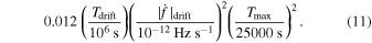
Since our largest initial ${T}_{\max }$ value is 25,290 s, the impact on the initial search and the upper limit of spin wandering at or below this level would be negligible. Note that even spin wandering, which posed no complication for the initial search, could potentially be a limitation for the follow-up procedure, where ${T}_{\max }$ is increased by a factor of 4 at level 2 and a factor of 16 at level 3. In any event, the impact depends on the level of spin wandering present, which is still an area of open research.

In the absence of a detection, we set upper limits on the strength of gravitational radiation from Sco X-1, as a function of frequency. We used as a detection statistic ${\rho }_{\max }$, the maximum statistic value observed in a $0.05\,\mathrm{Hz}$ band. We produced frequentist 95% upper limits via a combination of theoretical considerations and calibration with simulated signals, as explained in detail in Appendix A. The starting point was a Bayesian upper limit constructed using the expected statistical properties of the detection statistic and corrected for the reduction of sensitivity due to known lines. A series of simulated signal injections was then performed and used to estimate a global adjustment factor to estimate the amplitude at which a signal would have a 95% chance of increasing the ${\rho }_{\max }$ value in a band.

The procedure produced two sets of upper limits: a limit on h₀ including marginalization over the unknown inclination angle ι, and an unmarginalized limit on the quantity ${h}_{0}^{\mathrm{eff}}$ defined in Equation (2) to which the search is directly sensitive. The ${h}_{0}^{\mathrm{eff}}$ upper limit can also be interpreted as a limit on h₀ subject to the assumption of circular polarization (optimal spin orientation corresponding to $\cos \,\iota$ = ±1). It can be converted to a limit assuming linear polarization $\cos \,\iota =0$ by multiplying by $\sqrt{8}=2.83$. If we assume that the NS spin is aligned with the binary orbit (as one would expect for an NS spun up by accretion), $\iota \approx i\approx 44^\circ$, we obtain a limit on h₀, which is the ${h}_{0}^{\mathrm{eff}}$ upper limit multiplied by $1.35$.

We show the marginalized and unmarginalized upper limits of this search in Figure 5, along with the other upper limits on Sco X-1 set with O1 data: the unmodeled stochastic radiometer (Ballmer 2006) results of Abbott et al. (2017d) and the directed search results of Abbott et al. (2017f) using Viterbi tracking of a hidden Markov model (Suvorova et al. 2016) to expand the applicability of the sideband search (Messenger & Woan 2007; Sammut et al. 2014; Aasi et al. 2015b) over the whole run. The present results improve on these by a factor of 3–4, yielding a marginalized limit of ${h}_{0}\lesssim 2.3\times {10}^{-25}$ and an unmarginalized limit of ${h}_{0}^{\mathrm{eff}}\lesssim 8.0\times {10}^{-26}$ at the most sensitive signal frequencies between around $100\,\mathrm{Hz}$ and $200\,\mathrm{Hz}$. The marginalized 95% upper limits from Initial LIGO data (Abadie et al. 2011; Aasi et al. 2015b; Meadors et al. 2017) were all around $1.5\times {10}^{-25}$, so we have achieved an overall improvement of a factor of 6–7 from Initial LIGO to Advanced LIGO's first observing run, a combination of decreased detector noise and algorithmic improvements.

Zoom In Zoom Out Reset image size

We also plot for comparison the torque balance level predicted by Equation (4). The marginalized limits on h₀ come closest to this level at $100\,\mathrm{Hz}$, where they are within a factor of 3.4 of this theoretical level. In terms of ${h}_{0}^{\mathrm{eff}}$, the torque balance level depends on the unknown value of the inclination ι. For the most optimistic case of circular polarization ($\cos \,\iota$ = ±1), our unmarginalized limit is a factor of 1.2 above the torque balance level near $100\,\mathrm{Hz}$. Assuming linear polarization puts our limits within a factor of 3.5 of this level, and the most likely value of $\iota =44$ corresponds to an upper limit curve a factor of 1.7 above the torque balance level, again near $100\,\mathrm{Hz}$.

We have presented the results of a search for GWs from Sco X-1 using data from Advanced LIGO's first observing run. The upper limits on the GW amplitude represent a significant improvement over the results from Initial LIGO and are within a factor of 1.2–3.5 of the benchmark set by the torque balance model, depending on assumptions about system orientation. Future observing runs (Abbott et al. 2016f) are expected to produce an improvement in the detector strain sensitivity of $\gtrsim 2.5$. An additional enhancement will come with longer runs, as the amplitude sensitivity of the search scales as ${T}_{\mathrm{obs}}^{1/4}$. Algorithmic improvements that allow larger ${T}_{\max }$ with the same computing resources will also lead to improvements, as the sensitivity scales as ${T}_{\max }^{1/4}$ as well. A promising area for such an improvement is the use of resampling (Patel et al. 2010) to reduce the scaling of computing cost with ${T}_{\max }$ (G. D. Meadors et al. 2017, in preparation). (A similar method is used in the proposed semicoherent search described in Leaci & Prix 2015.) These anticipated instrumental and algorithmic improvements make it likely that search sensitivities will surpass the torque balance level over a range of frequencies (as projected in Whelan et al. 2015), and suggest the possibility of a detection during the advanced detector era, depending on details of the system such as GW frequency, inclination of the NS spin to the line of sight, and how close the system is to GW torque balance.

The authors gratefully acknowledge the support of the United States National Science Foundation (NSF) for the construction and operation of the LIGO Laboratory and Advanced LIGO as well as the Science and Technology Facilities Council (STFC) of the United Kingdom, the Max-Planck-Society (MPS), and the State of Niedersachsen/Germany for support of the construction of Advanced LIGO, and construction and operation of the GEO600 detector. Additional support for Advanced LIGO was provided by the Australian Research Council. The authors gratefully acknowledge the Italian Istituto Nazionale di Fisica Nucleare (INFN), the French Centre National de la Recherche Scientifique (CNRS), and the Foundation for Fundamental Research on Matter supported by the Netherlands Organisation for Scientific Research, for the construction and operation of the Virgo detector and the creation and support of the EGO consortium. The authors also gratefully acknowledge research support from these agencies as well as by the Council of Scientific and Industrial Research of India, Department of Science and Technology, India, Science & Engineering Research Board (SERB), India, Ministry of Human Resource Development, India, the Spanish Ministerio de Economía y Competitividad, the Vicepresidència i Conselleria d'Innovació Recerca i Turisme and the Conselleria d'Educació i Universitat del Govern de les Illes Balears, the National Science Centre of Poland, the European Commission, the Royal Society, the Scottish Funding Council, the Scottish Universities Physics Alliance, the Hungarian Scientific Research Fund (OTKA), the Lyon Institute of Origins (LIO), the National Research Foundation of Korea, Industry Canada and the Province of Ontario through the Ministry of Economic Development and Innovation, the Natural Science and Engineering Research Council Canada, Canadian Institute for Advanced Research, the Brazilian Ministry of Science, Technology, and Innovation, International Center for Theoretical Physics South American Institute for Fundamental Research (ICTP-SAIFR), Russian Foundation for Basic Research, the Leverhulme Trust, the Research Corporation, Ministry of Science and Technology (MOST), Taiwan, and the Kavli Foundation. The authors gratefully acknowledge the support of the NSF, STFC, MPS, INFN, CNRS, and the State of Niedersachsen/Germany for the provision of computational resources.

This paper has been assigned LIGO Document No. LIGO-P1600297-v24.

The method used to set the upper limits for each $0.05\,\mathrm{Hz}$ band in Section 5 consisted of three steps:

• 1.  
  An idealized 95% Bayesian upper limit was constructed using the posterior distribution $\mathrm{pdf}({h}_{0}^{2}| {\rho }_{\max })$ or $\mathrm{pdf}({[{h}_{0}^{\mathrm{eff}}]}^{2}| {\rho }_{\max })$.
• 2.  
  A correction factor was applied in each $0.05\,\mathrm{Hz}$ band to account for the loss of sensitivity due to omission of data impacted by known lines.
• 3.  
  A series of software injections was performed near the level of the 95% upper limit and used to empirically estimate a global correction factor for each upper limit curve based on the recovery or non-recovery of the injections.

A.1. Idealized Bayesian Method

The Bayesian calculation assumes that all of the ρ values for templates in the initial search represent independent Gaussian random variables with unit variance; one has mean ${[{h}_{0}^{\mathrm{eff}}]}^{2}\vartheta$ and the others have zero mean. Note that different regions of the orbital parameter space have different coherence times ${T}_{\max }$ and therefore $\vartheta$ values (cf. Equation (7)). The method produces a sampling distribution $\mathrm{pdf}({\rho }_{\max }| {[{h}_{0}^{\mathrm{eff}}]}^{2})$, marginalizing over the location of the signal in orbital parameter space.

This sampling distribution is used to construct a posterior distribution $\mathrm{pdf}({[{h}_{0}^{\mathrm{eff}}]}^{2}| {\rho }_{\max })$ assuming a uniform prior in ${({h}_{0}^{\mathrm{eff}})}^{2}$, and this is used to produce a 95% Bayesian upper limit on ${({h}_{0}^{\mathrm{eff}})}^{2}$ according to

$$\begin{eqnarray}&&{\int }_{0}^{({h}_{0}^{\mathrm{eff}}{)}_{95 \% }^{2}}d{[{h}_{0}^{\mathrm{eff}}]}^{2}\,\mathrm{pdf}({[{h}_{0}^{\mathrm{eff}}]}^{2}| {\rho }_{\max })=0.95.\end{eqnarray} \tag{ 12 }$$

To produce an upper limit on the intrinsic strength h₀, we assume a prior that is uniform in ${h}_{0}^{2}$ and $\cos \,\iota$, repeat the calculation above, and numerically marginalize over $\cos \,\iota$ to obtain a posterior $\mathrm{pdf}({h}_{0}^{2}| {\rho }_{\max })$.

A.2. Correction for Known Lines

Although we calculate a single $\vartheta$ value for each of the 18 search regions for a given $0.05\,\mathrm{Hz}$ band and use it in the calculation, the search can in principle have a different $\vartheta$ value for each template. This is because of the correction which omits data contaminated by Doppler-modulated known instrumental lines from the sum in Equation (7), a process that depends on the signal frequency f₀ as well as the projected orbital semimajor axis $a\,\sin \,i$. In each $0.05\,\mathrm{Hz}$ band, we estimate the distribution of the ratio of the actual $\vartheta$ to the band-wide $\vartheta ;$ the percentiles of this distribution are illustrated in Figure 6. We divide by the fifth percentile of this distribution (shown in the last panel of Figure 6) to produce corrected ${h}_{0}^{2}$ and ${({h}_{0}^{\mathrm{eff}})}^{2}$ upper limits.

Zoom In Zoom Out Reset image size

A.3. Empirical Adjustment from Software Injections

We performed a series of re-analyses of the data with a total of 754 simulated signals ("software injections") added to the data stream to validate the upper limits including the known line correction. The signals were generated over signal frequencies from 25 to $500\,\mathrm{Hz}$, some with h₀ set to some multiple of the marginalized 95% upper limit ${{h}_{0}}_{{\rm{UL}}}$, and others with ${h}_{0}^{\mathrm{eff}}$ set to some multiple of the unmarginalized 95% upper limit $h{{}_{0}}_{{\rm{UL}}}^{\mathrm{eff}}$. We defined "recovery" of the injection as an increase in the maximum detection statistic ${\rho }_{\max }$ compared to the results with no signal present. (Follow-up of the recovered injections that crossed the relevant ρ threshold was also performed as a way of testing our follow-up procedure, as described in Section 4.) We find that the fraction of signals of each type recovered when the injection is done at the upper limit level to be slightly below the expected 95%.¹⁵⁶ This is to be expected, as there are various approximations in the method, such as the tolerated mismatch in the initial parameter space grid and the acceptable loss of S/N due to finite-length SFTs, which should lead to an S/N slightly less than that predicted by Equation (6).

To estimate empirically the amount by which the upper limits should be scaled to produce a 95% injection recovery efficiency, we apply the method described in Whelan (2015) and used to produce the efficiency curves in Messenger et al. (2015). We posit a simple sigmoid model where the efficiency of the search as a function of signal strength x is assumed to be $\varepsilon {(x;\alpha ,\beta )=(1+{e}^{-\alpha (\mathrm{ln}x-\beta )})}^{-1}$ and construct the posterior from the recovery data (D_i = 1 if the signal i was recovered, 0 if not):

$$\begin{eqnarray}&&\begin{array}{l}\mathrm{pdf}(\alpha ,\beta | \{{D}_{i}\},\{{x}_{i}\})\propto \displaystyle \prod _{i}\varepsilon {({x}_{i};\alpha ,\beta )}^{{D}_{i}}\\ \quad \times \,{(1-\varepsilon ({x}_{i};\alpha ,\beta ))}^{1-{D}_{i}}\mathrm{pdf}(\alpha ,\beta ).\end{array}\end{eqnarray} \tag{ 13 }$$

With sufficient data, the prior should be irrelevant, but we take a noninformative prior $\mathrm{pdf}(\alpha ,\beta )\propto {\alpha }^{-1}$ and define the signal strength x as the h₀ or ${h}_{0}^{\mathrm{eff}}$ of the injection divided by the corresponding upper limit. We can then construct, at any signal level x₀, the posterior on the efficiency ${\varepsilon }_{0}=\varepsilon ({x}_{0};\alpha ,\beta )$, marginalized over α and β:

$$\begin{eqnarray}&&\begin{array}{l}\mathrm{pdf}({\varepsilon }_{0}| \{{D}_{i}\},\{{x}_{i}\})={\displaystyle \int }_{0}^{\infty }d\alpha {\displaystyle \int }_{-\infty }^{\infty }d\beta \,\mathrm{pdf}(\alpha ,\beta | \{{D}_{i}\},\\ \,\times \{{x}_{i}\})\,\delta ({\varepsilon }_{0}-\varepsilon ({x}_{0};\alpha ,\beta )).\end{array}\end{eqnarray} \tag{ 14 }$$

The posterior distributions of efficiency are shown in Figure 7. We define the correction factor to be the x₀ at which the expectation value ${\int }_{0}^{1}d{\varepsilon }_{0}\,\mathrm{pdf}({\varepsilon }_{0}| \{{D}_{i}\},\{{x}_{i}\})$ crosses 95%.

Zoom In Zoom Out Reset image size

A total of eight sets of injections were performed, four with h₀ at a specified multiple of ${{h}_{0}}_{{\rm{UL}}}$, and four with ${h}_{0}^{\mathrm{eff}}$ at a specified multiple of $h{{}_{0}}_{{\rm{UL}}}^{\mathrm{eff}}$. The multipliers were 1.0, 1.1, 1.2, and a random value between 1.1 and 2.0 chosen from a log-uniform distribution. For the unmarginalized ${h}_{0}^{\mathrm{eff}}$ upper limit, we use all eight sets of injections, 754 in total and find the expectation value of the efficiency crosses 95% at ${h}_{0}^{\mathrm{eff}}/h{{}_{0}}_{{\rm{UL}}}^{\mathrm{eff}}\approx 1.21$. This factor has been applied to $h{{}_{0}}_{{\rm{UL}}}^{\mathrm{eff}}$ to produce the upper limits in Figure 5.

For the marginalized h₀ upper limit, we must restrict ourselves to the four injection sets which specified ${h}_{0}/{{h}_{0}}_{{\rm{UL}}}$. This is because our search is primarily sensitive to ${h}_{0}^{\mathrm{eff}}$, and specifying ${h}_{0}^{\mathrm{eff}}$ while choosing the inclination angle ι randomly implies anticorrelations between h₀ and $| \cos \,\iota |$. Signals with high h₀ values will tend to be those with unfavorable polarization, and therefore not be any easier to detect. Using the 376 applicable injections, we estimate the 95% efficiency at ${h}_{0}/{{h}_{0}}_{{\rm{UL}}}\approx 1.44$ and use this factor when generating the final upper limit shown in Figure 5. Note that this is less well determined than the factor for the unmarginalized ${h}_{0}^{\mathrm{eff}}$ upper limit. This is both because of the smaller number of injections used and because h₀ correlates less well with detectability than ${h}_{0}^{\mathrm{eff}}$. However, the upper limit curve for h₀ is very close to the unmarginalized upper limit assuming linear polarization ($\cos \,\iota =0$), which is consistent with the expectation that the 95% upper limit will be dominated by this worse-case scenario.

As noted in Table 2, the range of $a\,\sin \,i$ values searched was chosen based on preliminary information from Wang (2017), which constrained the projected orbital velocity K₁ to lie between 10 and $90\,\mathrm{km}\,{{\rm{s}}}^{-1}$. This was subsequently refined to between 40 and $90\,\mathrm{km}\,{{\rm{s}}}^{-1}$. For comparison, we recomputed the upper limits, discarding the results of searches with a sin i ≤ 1.44 lt-s, corresponding to the nine bottom-most parameter space cells shown in Figure 2. The results were not significantly different (for instance, they were barely noticeable on plots like Figure 5), but for illustration we plot in Figure 8 the ratio of the two sets of upper limits. A bigger impact of the refined parameter space will be seen in future runs, when computing resources can be concentrated on the allowed range of $a\,\sin \,i$ values.

Zoom In Zoom Out Reset image size