


Abstract
We present a path forward on a long-standing issue concerning the flux of small and slow meteoroids, which are believed to be the dominant portion of the incoming meteoric mass flux into the Earth's atmosphere. Such a flux, which is predicted by dynamical dust models of the Zodiacal Cloud, is not evident in ground-based radar observations. For decades this was attributed to the fact that the radars used for meteor observations lack the sensitivity to detect this population, due to the small amount of ionization produced by slow-velocity meteors. Such a hypothesis has been challenged by the introduction of meteor head echo (HE) observations with High Power and Large Aperture radars, in particular the Arecibo 430 MHz radar. Janches et al. developed a probabilistic approach to estimate the detectability of meteors by these radars and initially showed that, with the current knowledge of ablation and ionization, such particles should dominate the detected rates by one to two orders of magnitude compared to the actual observations. In this paper, we include results in our model from recently published laboratory measurements, which showed that (1) the ablation of Na is less intense covering a wider altitude range; and (2) the ionization probability,  , for Na atoms in the air is up to two orders of magnitude smaller for low speeds than originally believed. By applying these results and using a somewhat smaller size of the HE radar target we offer a solution that reconciles these observations with model predictions.
Export citation and abstract BibTeX RIS
1. Introduction
The source of meteoroids originating from the Sporadic Meteor Complex (SMC) is composed of Interplanetary Dust Particles (IDPs) forming the Zodiacal Dust Cloud (ZDC). The particles in this cloud, which originate from the collision of asteroids and disintegration of comets, have orbital characteristics that have evolved significantly from the moment of ejection and thus, a direct link to their original progenitor body is generally very difficult to establish. Nevertheless, these IDPs evolve in such a way that they can be categorized in a general manner in relation to the type of bodies they originated from. Specifically, from the point of view of ground-based radar and optical observations, the SMC is composed of six main directional enhancements of the meteor radiants (i.e., orbital families). These apparent sources are known as the North and South Apex (NA and SA), composed mainly of dust from long-period comets (Sekanina 1976; Nesvorný et al. 2011b); the Helion and Antihelion (H and AH), composed of dust from short-period comets (Hawkins 1956; Weiss & Smith 1960; Nesvorný et al. 2010, 2011b); and the North and South Toroidal (NT and ST), which have been recently associated with dust from Halley-type comets (HTCs; Pokorný et al. 2014). Recently, several efforts have been made in modeling these sources using dynamical models of dust evolution from different cometary families and constrain them with both spaceborne and ground-based observations (Nesvorný et al. 2010, 2011a, 2011b; Pokorný et al. 2014). In particular, the modeling of the short-period Jupiter Family Comets (JFCs; Nesvorný et al. 2010, 2011a), hereafter referred as to ZoDy, which mostly form the H and AH sources, have raised some controversies. These arise from the need for a predicted large flux of small (∼10 μg) particles with slow velocities (<15 km s−1) contributing to the total meteoric flux into the Earth atmosphere in order to model the infrared spectral shape of the ZDC measured by the InfraRed Astronomy Satellite. As a consequence, and due to the fact that such a population is not evident in ground-based radar observations, the authors concluded that most of these particles must be undetected by radars.
The assumption that meteor radars cannot be used to retrieve the mass flux reliably, due to a lack of sensitivity to the majority of incoming particles, has been used for decades since the seminal work by Hughes (1978), who showed a large difference in detections by specular trail meteor radars, as compared to those from satellite dust impact detector measurements. Similarly, Nesvorný et al. (2011a), using results from the Canadian Meteor Orbit Radar (CMOR; Webster et al. 2004) and the Advanced Meteor Orbit Radar (AMOR; Baggaley et al. 1994), argued that in fact most of the input flux is undetected by ground-based radars. This hypothesis has been historically well justified because it has been based on radars that lack the sensitivity to observe the particle masses ( μg) and velocities (
 km s−1) that appear to be dominant in the incoming flux. However, the hypothesis has become more difficult to support with the introduction, over two decades ago, of routine meteor head echo (HE) detections with the more sensitive High Power and Large Aperture (HPLA) radars. Specifically, the hypothesis of an undetected flux becomes extremely challenging to maintain for the case of the 430 MHz Arecibo Radar in Puerto Rico, the most sensitive radar used for meteor observations to date.
Motivated by these findings and challenges, we reported in Janches et al. (2014), hereafter referred as J14, and Janches et al. (2015b), hereafter referred as J15, a new approach that calculates the probability of detecting meteor HEs as a function of particle mass (m), incoming velocity (V), and entry angle (α) by several HPLA radars and thus we explored the sensitivity of these instruments to various mass/velocity particle populations. Specifically, in J15, we compared predicted and observed meteor rates and velocity distributions detected by three different HPLA radar systems, assuming the input to be those fluxes reported by Nesvorný et al. (2011a). Besides the Arecibo radar, we utilized data from the less sensitive 440 MHz Poker Flat Incoherent Scatter Radar (PFISR; Sparks et al. 2009) in Alaska and the 46 MHz Middle and Upper Atmosphere Radar (MU; Pifko et al. 2013) in Japan. Furthermore, we performed these comparisons with a flux model that assumes a particle Size Frequency Distribution (SFD) function given by Fixsen & Dwek (2002):
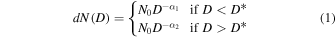
where N0 is a normalization constant,  and
and  are the slope index and D* is a free parameter. Originally, Nesvorný et al. (2011a) proposed D* = 100 μm to match the results derived from the measurements obtained with the Long Duration Exposure Facility (LDEF; Love & Brownlee 1993). However, in J15 we also investigated the case of D* = 30 μm derived from Planck satellite observations (Ade et al. 2014), which provided better agreement to the radar observations because they implied that the characteristic particle mass of the incoming flux is about a factor of 27 smaller than the original ZoDy, and thus more easily made "undetectable."
Finally, as discussed in J14 and J15, the radar detectability of meteors has typically been estimated by using a crude average of the ionization probability  (Jones 1997; Close et al. 2002, 2005). Using a single composition body assumption (i.e., one value of β) can result in different, and perhaps incorrect, interpretations of radar observed features. For example, sudden and sharp increases in the observed S/N curves observed with the ARPA Long-range Tracking and Instrumentation Radar (ALTAIR) facility were interpreted as fragmenting events by Campbell-Brown & Close (2007), who used a single value of the ionization probability coefficient in their ablation model. However, using the Chemical Ablation Model (CABMOD), Janches et al. (2009) demonstrated that such features are explained by the specific ablation of volatiles off the meteoroid body. This quantity, which gives a measure of the electron production rate, depends on meteoroid mass, composition, and velocity (see Section 2.2), and can vary up to two orders of magnitude depending on the meteoroid ablating constituent under consideration (Vondrak et al. 2008). Our modeling treatment overcomes this limitation via the utilization of CABMOD developed by Vondrak et al. (2008), which considers the full treatment of the ablation and ionization of the individual chemical elements. Specifically, we explored two sets of values for
  : (1) those derived by Jones (1997),6
which are based on experiments reported in Friichtenicht & Becker (1973) involving the firing of high-velocity Fe particles into a chamber of air at low pressure and measuring electron production along the particle track; and (2) a re-estimation of
: (1) those derived by Jones (1997),6
which are based on experiments reported in Friichtenicht & Becker (1973) involving the firing of high-velocity Fe particles into a chamber of air at low pressure and measuring electron production along the particle track; and (2) a re-estimation of  as a function of collision energy by utilizing measurements of the ionization cross section of K atoms in collision with O2 and N2 over the full range of collision energies reported by Cuderman (1972).
The results reported in J14 and J15 showed that, even by extensively revising the widely used ionization coefficient of ablating meteors reported by Jones (1997) as well as utilizing an SFD weighted toward smaller particles by adopting D* = 30 μm, the JFC dust fluxes predicted by ZoDy are significantly larger than those actually observed. The reported results showed that the observed distributions for the case of AO and PFISR, when the original value of  is considered, disagree with the model predictions by one to two orders of magnitude. For the case of MU, even though the reported results showed that the predictions are approximately the same values as the observations, they disagree with the fact that the majority of the detections are from meteors originating from the Apex source (i.e., from long-period comets), which are currently not included in ZoDy. In order to find agreement, the predictions should not exceed more than ∼30% of the observations since ZoDy particles are those with radiants from the Helion and Antihelion directions (Fentzke & Janches 2008; Fentzke et al. 2009; Pifko et al. 2013). Furthermore, the predicted distributions for PFISR and MU fall below the observed ones, as would be expected if the ZoDy flux are mostly undetected and would represent less than a third of the detections, only when we utilize the revised
  . However, it is also suggested that the revision of
  was too extreme when looking in depth at the PFISR and MU results, in particular, the peak of the predicted occurrence rate. Nevertheless, the reported test was a clear indication that in order to find an agreement between ZoDy and sensitive HPLA meteor observations requires a re-examination not only of our knowledge on the ablation, ionization, and radar detection processes but also the physical assumptions in the ZDC model itself.
Three recent developments have compelled us to revisit and further explore the detectability (or lack thereof) of these small and slow particles. The first development was reported by Thomas et al. (2016), who measured  for Fe in N2 and air, confirming the much earlier measurements by Friichtenicht et al. (1967) and Friichtenicht & Becker (1973), and thus corroborating the conclusion that the revised values of
  utilized in J14 and J15 were in fact too extreme. Second, Carrillo-Sánchez et al. (2016), using an improved version of CABMOD (see Section 2.1), further constrained ZoDy with observations of vertical fluxes of Na and Fe determined from ground-based LIDAR observations, as well as the flux of spherules estimated in the South Pole, showing the need for a large flux (∼34 t day−1) of small and slow particles representing about 80% of the incoming mass flux, in good agreement with Nesvorný et al. (2011a). The third and final development involves recent results from a newly developed laboratory Meteor Ablation Simulator (MASI; Bones et al. 2016). Specifically, Gómez Martín et al. (2017) used MASI to produce vaporization profiles and test them against CABMOD-predicted deposition profiles for Na, Fe, and Ca in order to improve the model. In particular, the authors focused on better reproducing the specific shape of the elemental ablation profiles, in particular those of alkali constituents, which play a crucial role in the detectability of the small and slow portion of the incoming IDPs as shown in J14. Details of these developments are presented in Section 2. Thus in this work we concentrate on exploring the last three specific parameters, which play a major role in the ability to detect the particles of interest. These are (1) the specific ability to detect ionization from volatile (i.e., Na) atoms, given the latest laboratory measurements, which will be the main constituents ablating from slow particles; (2) the size of the meteor HE; and (3) the potential angular dependence of the HE detection.
2. Model Updates and Results
In J14 and J15 we developed a methodology aimed at constraining models of the ZDC meteoroids, based on ground-based HPLA meteor HE radar observations (Janches et al. 2014, 2015b). The methodology employs a comprehensive treatment of the chemical and physical process that meteoroids undergo upon atmospheric entry given by CABMOD (Vondrak et al. 2008; Janches et al. 2009). Specifically, CABMOD provides the altitude profile for the production of various metallic atoms and electrons as a function of a particle's m, V, and α as it penetrates the atmosphere. In particular, the altitude profile of electron production,  , is then used together with an HE model, the radar equation and a parameterization of the radar beam pattern to calculate the meteor signal-to-noise ratio (S/N). The model assumes that the HE is an ensemble of electrons with radius equal to the atmospheric mean free path (MFP), following the results reported by Mathews et al. (1997). We applied our approach for estimating the detection probability of meteors by three different HPLA radar systems with significantly different characteristics, and showed how the different systems detect different parts of the incoming populations. However, the main result is that even with the least sensitive MU radar system, the current ZDC model overpredicts the radar observations of detected rates and velocity distributions and a satisfactory reconciliation between ZoDy and HPLA radar observations could not be achieved thus far. In this section we explore two physical effects concerning the detectability of the HE concerning the dependency of ablated constituent with meteoroid velocity and the size of the HE (i.e., plasma cloud surrounding the meteoroid). In Section 2.4 we discuss the results derived from upgrading our model based on these effects, their implications regarding the physical characteristics of the plasma generating the HE, as well as the consequences of introducing the probability of detection as a function of the meteoroid's speed and mass.
2.1. CABMOD Improvements
The mass-loss rate in CABMOD is calculated using the Langmuir treatment of evaporation kinetics (Vondrak et al. 2008), which assumes that the rate of evaporation into a vacuum is equal to the rate of evaporation needed to balance the rate of uptake of a species i in a closed system. The rate of mass release of species i with molecular weight  , from a particle of area S and a temperature T, is given by the Hertz–Knudsen expression

where the subscript A refers to thermal ablation; kB is the Boltzmann constant, pi is gas-liquid equilibrium vapour pressure, and  is the apparent evaporation coefficient, which is equal to the probability that the molecule is retained on the surface, or within the particle, after collision. Safarian & Engh (2013) concluded that
  is unity for pure metals but may be lower than 1 in silicate melts (Alexander et al. 2002) because diffusion from the bulk into the surface film may become rate-limiting. Due to the lack of experimental data, the apparent evaporation coefficient for each metal is assumed to be the same for all the compounds of the bulk, such that
  (Vondrak et al. 2008). The range of temperature where the solid and the liquid are in equilibrium is treated by applying a phase transition factor f(T) (Gómez Martín et al. 2017), which is represented by a sigmoid temperature dependence weighting that varies between 0 and 1:

where τ is a constant that characterizes the width of the sigmoid profile and Tc is the temperature such that  . The values Tc = 1800 K and τ = 14 K are prescribed for the olivine Fa50 solid–liquid equilibrium temperature range, meaning essentially that
  and
and  (Vondrak et al. 2008).
The previous version of CABMOD (hereafter referred as CABMOD v1, Vondrak et al. 2008) simulated poorly the width of the Na and Fe peaks, and the magnitude of the Ca ablation relative to Na (see Figure 14 of Gómez Martín et al. 2017), which is an important consideration since it is the instantaneous properties of single meteors that play a primary role for radar detection (Janches et al. 2014). In a first attempt to improve the agreement between CABMOD and MASI, the model was upgraded with the latest version of the MAGMA code (Fegley & Cameron 1987), which includes revised data for Na and K alumino-silicates (Holland & Powell 2011). Revision of the thermodynamics of Na resulted in lower equilibrium vapour pressures and thus in a lower evaporation rate, which fits better the high-temperature tail of the Na pulses measured by MASI. A temporary solution for the Na profile has been found by increasing the width of τ (which defines the width of the temperature dependence) in the transition between the liquid and solid phase. Due to its low ionization potential and high volatility, ablated Na is a major contributor to radar detectability, in particular for the slow-velocity particles.
The effect that the new version of CABMOD (hereafter referred to as CABMOD v2, Gómez Martín et al. 2017) introduces to the calculation of  is shown in Figure 1. The top panel of this figure shows the altitude profile of
  for a particle with m = 10 μg, α = 45° entering the atmosphere at two velocities: 14 km s−1 (blue lines) and 40 km s−1 (black lines). The bottom panel shows the results for the case of a particle with m = 1 μg. The solid lines represent the electron density calculations using the original version of CABMOD presented in J14 and J15 while the dotted lines utilize the new one. The dashed lines represent the results derived from further improvements discussed in Section 2.2. The figures show that the main differences between CABMOD v1 and v2 is a wider altitude range over which electrons resulting from the ablation of Na are produced. Also, the peak production occurs at lower altitudes. The magnitude of the peak is somewhat lower but not significantly so. For the case of smaller masses, electrons resulting from the ablation of the main constituents is somewhat larger than for the case of the CABMOD v1, which likely results from the overlap with the wings of the broader CABMOD v2 alkali peaks, since no changes have been made in CABMOD related to Fe, Mg, or Si. Overall, the differences introduced by using the CABMOD v2 will not produce significantly different results in the overall detectability of meteors than those presented in J14 and J15.

Figure 1. Electron production profiles as a function of altitude predicted by CABMOD. The top panel displays the case for m = 10 μg while the bottom is for the case of m = 1 μg. The black lines display the cases for fast meteors (V = 40 km s−1), while the blue lines are the cases for slow particles (V = 14 km s−1).
Download figure:
Standard image High-resolution image2.2. The Role of Na in the Detectability of the Meteor HE
Estimating the rate of electron production from a meteoroid requires the ionization efficiencies  of the individual elements once they ablate and collide with air molecules (O2 or N2) at hyperthermal velocities. Unfortunately, there is relatively little laboratory data available. In our previous study reported in J14 and J15 we used the ionization cross section of K atoms in collision with O2 and N2 over a large range of collision energies (Cuderman 1972) as a reference point. We used these results because this was the only metallic atomic species for which experimental data with both collision partners over a wide collision energy existed. The most challenging aspect of these beam-gas experiments is determining the absolute cross section for ionization. Although Cuderman (1972) appears to have carried out a careful study, we have now concluded that the cross sections were underestimated, based on very recent results reported by Thomas et al. (2016). The authors measured
  for Fe in N2 and air by reproducing the experimental arrangement and results reported by Friichtenicht et al. (1967). Figure 2 illustrates
  (Fe) as a function of impact velocity, where the red line represents the results derived by Friichtenicht et al. (1967) and later utilized by Jones (1997), the black line is the recent measurements by Thomas et al. (2016), and the blue and green lines are the values obtained for K and Fe, respectively, using the measurements of Cuderman (1972) and reported in J14. At a representative velocity of 20 km s−1 (vertical dash line in Figure 2),
  (Fe in air) = 0.03. In contrast, using
  (K in air) as the reference point from Cuderman (1972) indicates that
  (Fe in air) is only 0.0015 (Janches et al. 2014), roughly a factor of 20 smaller. We therefore now use the new measurements of
  (Fe) from Thomas et al. (2016) as the reference point for the present study, and estimate
  for the other metals using the following procedure (also described in J14).

Figure 2. Comparison of  as a function of velocity for Fe atoms on air from the different estimates utilized throughout this work.
Download figure:
Standard image High-resolution imageThe ionization probability for the first collision after ablation,  , is expressed as a function of collision V by the analytic expression of Jones (1997)

where V0 is the threshold velocity, given by

where Me and ψ are the mass and ionization potential of the atom, respectively, e is the electronic charge, Ma is the molecular mass of O2 or N2, and c is a fitted parameter. For Fe in air, c = 1.97 × 10⁻⁵ (km s−1)−2.8, and V0 = 8.91 km s−1.  is then increased to allow for ionization through subsequent collisions of the metal atom as it loses momentum (Jones 1997):

These new results, in principle, worsen the agreement between ZoDy predictions and HPLA observations because the larger  values will produce stronger radar returns signals. However, as discussed in J14 (see discussion for Figure 9 in Janches et al. 2014), the detectability of the slow and small particles, which are the particles in question, will strongly depend on the ability to detect electrons produced from the ablation of alkali atoms (i.e., K and Na), as they are the elements that will ablate more easily off the meteoroid's body according to differential ablation (Vondrak et al. 2008; Janches et al. 2009).
In order to determine  for Na and other meteoric metals, we first estimate the maximum interaction distance between a metal atom and a collision partner (O2 or N2) as the curve-crossing (or harpoon) distance, Rc given by7

where γ is the vertical electron affinity of O2 and N2, which is close to zero and thus Rc is inversely proportional to the ionization potential of the metal atom ψ. The ionization cross section should then scale as Rc2 (i.e., a target of radius Rc), and hence to the inverse square of the ionization potential ( ). The premise of the harpoon mechanism is that the electron transfer occurs at a distance where the energy involved (ionization potential of the metal atom minus the electron affinity of the O2 or N2) is balanced by the resulting Coulomb attraction of the metal ion and the O2-or N2-anion (Smith 1980).
The probability of ionization,  , in Equation (4) is (to the first order) proportional to c, since the second term in the denominator is less than 1 for
  km s−1, and less than 3 even at the highest V of 72 km s−1.
  and thus c are proportional to the cross section for ionizing collisions. Hence, c is proportional to
  and thus knowing c(Fe), the c parameter can be estimated for other metals as

Using Equation (8), the c parameter for Na, K, Mg, Si, and O can then be estimated by multiplying the value of 1.97 × 10⁻⁵ (km s−1)−2.8 for Fe (in air) by factors of 3.30, 2.36, 1.06, 0.94, and 0.34, respectively. V0 in Equation (5) is estimated for each element from its respective ψ (Equation (5)). The values of c and V0 for calculating  using Equations (4) and (6) are listed in Table 1, and the resulting curves of
  versus V0 in air are illustrated in Figure 3. To check on this procedure we compare our results with existing experimental data for Na + O2 and N2 collisions. Bydin & Bukteev (1960) showed that at collision velocities below 50 km s−1, the ionization cross section for O2 is more than 70 times larger than for N2, so that air collisions with N2 will produce very few electrons. Moutinho et al. (1971) measured an absolute cross section for electron production in O2 of 0.4 Å2. This may be compared with a capture cross section of 15.4 Å2 computed from long-range capture theory, using the experimental polarizabilities and ionization potentials for Na and O2 to calculate the C6 parameter (=3.3 × 10−77 J m6) for the London intermolecular potential (Smith 1980). This implies
  (Na in O2) = 0.4/15.4 = 0.026. In air this will be reduced by a factor of four (since
  (Na in N2) is so much smaller). At a low collision velocity,
  (Na) from Equation (6), so
  (Na in air) = 0.0082. As shown in Figure 3, this experimental point from Moutinho et al. (1971) is in very good agreement with the value of
  (Na in air) based on the measurement of
  (Fe in air; Figure 2 and Thomas et al. 2016). In addition, a preliminary comparison of this methodology with recent measurements of
  for Al suggests that the calculation matches the measurements within a factor of five (DeLuca & Sternovsky 2016, personal communication).

Figure 3.
 as a function of velocity for various elements estimated using
  for Fe atoms in air measured by Thomas et al. (2016) as a reference.
Download figure:
Standard image High-resolution imageTable 1.
Fitted Parameters for Calculating  as a Function of V
| Atom | c/(km s−1)−2.8 | V0/(km s−1) |
|---|---|---|
| K | 6.49 × 10⁻⁵ | 7.0 |
| Na | 4.63 × 10⁻⁵ | 8.6 |
| Mg | 2.09 × 10⁻⁵ | 10.6 |
| Fe | 1.97 × 10⁻⁵ | 8.9 |
| Si | 1.85 × 10⁻⁵ | 10.6 |
| O | 6.62 × 10⁻⁶ | 16.0 |
Download table as: ASCIITypeset image
A comparison of the new proposed  (Na) with those used in Vondrak et al. (2008) and Janches et al. (2014) is shown in Figure 4. The top panel of this figure compares the revised values of
  (Na in air) recalculated using
  (Fe in air) measured by Thomas et al. (2016) as a reference point (black line) with those originally utilized by Vondrak et al. (2008; red line) and the revised values reported in J14 using K atoms in collision with O2 and N2 over a large range of collision energies (Cuderman 1972) as a reference point (blue line). The bottom panel of Figure 4 shows the ratio between the different results. It can be seen from this figure that the revision reported in J14 significantly decreased
  (Na in air) over the entire velocity range, while the results from the approach proposed here mostly affect the detectability of slower particles (V < 30 km s−1).

Figure 4. Top panel:  as a function of velocity for Na atoms impacting air for the various versions of the detectability model used in this and previous work. Bottom panel: ratio of
  as a function of velocity for Na atoms impacting air used by Vondrak et al. (2008) to the revisions reported by J14 and the one reported in this work.
Download figure:
Standard image High-resolution imageThe degree of change that the new  (Na in air) introduces to the calculation of
  is represented by the dashed lines in Figure 1. From these panels it can be seen that at low velocities, the new
  (Na in air) introduces up to a two-order-of-magnitude decrease in the amount of electrons produced, mostly by the ablation of Na, while at higher speeds, the change is about a factor of 10. As expected, the changes are greater for smaller sizes. In particular, as can be seen in the blue lines of the bottom panels, since alkalis are basically the only elements ablating and producing electrons for small and slow particles, the new estimation of
  (Na in air) will have a critical effect in the detectability of the incoming flux. This can be seen in Figure 5 where the modeled and observed rates (top panel) and radial (i.e., line of sight) velocity distributions (bottom panel) are displayed. The black line histograms are the observations, the blue lines are the original results presented in J14, which uses CABMOD v1 and the original estimate of β(Na) (Vondrak et al. 2008), and the red line shows the results derived using the new version of CABMOD as well as the new calculation of
  (Na in air). The rates and velocity distributions are estimated using ZoDy, constrained by the Planck satellite measurements (i.e., D* = 30 μm). As can be seen from this figure, while our treatment with the new modifications still overpredicts the observed quantities, the agreement is closer by an order of magnitude. More particles with slower radial velocities are filtered out, as seen in the lower panel. Another new effect is that at about 04:00 a.m. (28 hr from midnight of July 15th), the detected rates experience a decrease, in agreement with the observations, but in contradiction with our previous results, which showed an increase in the detected rates.

Figure 5. Top panel: comparison between predicted detected meteor rates assuming ZoDy to be the incoming flux and those observed by Arecibo. Bottom panel: comparison between predicted radial velocities of detected meteors assuming ZoDy to be the incoming flux and those observed by Arecibo. The blue lines represent the original predictions reported in J14 and red lines represent the revised predictions using the new version of CABMOD and the new estimate of  as a function of velocity for Na atoms presented in this work.
Download figure:
Standard image High-resolution image2.3. Size of Meteor HE
As discussed earlier, our detectability model requires a physical assumption of the radar scattering target or HE, which is commonly believed to be "a ball of plasma" traveling at or near the speed of the meteoroid (Mathews et al. 1997; Janches et al. 2000; Close et al. 2002). In our current model of the HE radar cross section (RCS) reported in J14 and J15, we followed the results reported by Mathews et al. (1997) by assuming it to be an ensemble of electrons given by

where re is the classical electron radius ( m) and
  is the altitude profile of electron production, provided by CABMOD. This model of the HE assumes that the scattered radio waves are the result of all electrons (single) scattering in-phase, producing a scattered power that is a function of Ne2. This is valid while the characteristic size of the ensemble is small compared with the radar wavelength, and so we assume also that, at a given time, the diameter of the cloud of electrons producing the HE is of the order of the atmospheric MFP multiplied by a scale factor F given by8

where λ is the radar wavelength. The scale factor F accounts for the fact that for meteor plasma larger than a quarter-wavelength, the radar wave cannot completely penetrate the plasma, and so the scattering ability of the interior electrons is reduced. Equation (9) is then utilized with the radar equation and a parameterization of the radar beam pattern to calculate the meteor S/N (Janches et al. 2014, 2015b).
In this section we first examine how well this approximation fares with a recent and more comprehensive model of the meteor HE, and determine what improvements can be made to find reconciliation between radar observations and ZoDy. Specifically, we will compare our results to the model reported by Marshall & Close (2015), who have developed a three-dimensional Finite-difference Time-domain (FDTD) model to investigate the scattering of radar waves from the meteor HE, treating it as a cold, collisional, magnetized plasma. Solving Maxwell's equations and the Langevin equation simultaneously and self-consistently in and around the plasma, the model explores the dependence of the meteor RCS with physical variables such as plasma densities, meteor HE scale sizes, and wave frequencies. The authors found that the computed RCS disagrees with previous analytical theory at certain meteor HE sizes and densities; in some cases the discrepancies could be over an order of magnitude. The authors concluded that for overdense meteors, the meteor head RCS is given by the overdense area of the meteor, defined as the cross-section area of the part of the meteor where the plasma frequency exceeds the wave frequency. For underdense meteors, the model provides a monotonic relationship between the meteor plasma size and peak density and the resulting RCS. These results provide a physical measure of the meteor HE size and density that can be inferred from measured RCS values from ground-based radars.
Figure 6 shows the absolute difference between the RCS calculated using the FDTD model developed by Marshall & Close (2015) and the coherent scattering model utilized thus far by our approach. It can be seen from this figure that the ensemble of electrons model is in reasonably good agreement with the FDTD simulations for the range of masses between 0.01 and 1000 micrograms, where at low velocities the RCS from the FDTD simulations is at most a factor of 0.1 smaller than that resulting from the coherent scattering approach. The FDTD model assumes a Gaussian electron density distribution (Close et al. 2012), and from these results it appears that coherent scattering works reasonably well as an approximation when the HE is underdense, that is, the peak plasma frequency ( ) is lower than the radar frequency (
 ). For this case, the head plasma should emulate coherent scattering as the radar wave is able to penetrate the plasma and be seen by all of the head plasma electrons, which each scatter the radar wave independently and coherently. On the other hand, when the HE is overdense, the radar wave hits a "wall" where
  , and the head plasma reflects the wave; only under those circumstances, Marshall & Close (2015) report an RCS
  , where rp is the overdense radius. The calculated electron densities from CABMOD result in normalized plasma frequencies that are smaller than 3 and actually generally smaller than 1. Thus we observe that the relatively simple coherent scattering parameterization approximates reasonably well the results of the general FDTD model for the particular case of underdense HEs, which applies to the range of dominant ZoDy meteoroid masses and speeds. Therefore the choice of the HE scattering model used here is not expected to yield very different results.

Figure 6. Difference between RCS values derived using the FDTD model developed by Marshall & Close (2015) and the ensamble of electrons proposed by Mathews et al. (1997) and utilized in our detectability model, as a function micrometeoroid mass and velocity.
Download figure:
Standard image High-resolution imageFinally, we explore in our model the validity of using the atmospheric MFP, scaled by Equation (10) as the characteristic size of the HE, as well as any potential angular dependence the detection of this target may have. We compare our results with those used by previous works, in particular that reported by Close et al. (2004), who also argued that the physical size of head plasma must scale approximately with the atmospheric MFP because the electrons detected by the radar are contained within a region of ionization produced by the ablation of the meteoroid resulting from collisions with neutral air molecules. Therefore, as the MFP decreases with decreasing altitude, so would the size of the HE. In addition, there is a transition region between the atoms and ions being released from a meteoroid and expanding largely without deflection to a point where the expansion occurs at a slower diffusive rate. Jones (1995) defined this distance as the initial trail radius and estimate it as

where V is the meteoroid velocity in km s−1 and n is the background number density at the altitude at which the HE is detected. We refer hereafter to Equation (11) as the Jones formula or Jones radius. Below, it deviates from MFP and can be up to a factor of five smaller. In fact, Close et al. (2004), using simultaneous VHF/UHF detections obtained with the ALTAIR system, estimated the head radius to be  . Figure 7 displays the ratio of the Jones radius to MFP. The Jones radius is calculated at the altitude at which ablation is maximum according to CABMOD. In this figure, the Jones radius is calculated with the 0.023 scale factor introduced by Close et al. (2004) and it can be seen that the MFP is a factor of ∼5 larger than the head radius at the lowest speed, and on average a factor of 3 times larger than the head radius below 20 km s−1 at the altitude at which the ablation is maximum according to CABMOD. This comparison suggests that using the MFP or Jones radius does not change the results significantly. Furthermore, from Figure 7 of Marshall & Close (2015), it can be seen that the RCS derived from Close et al. (2004) analytical model for a given radius is larger than the one derived by the FDTD simulations. This suggests that the Jones radius correction (0.023) derived by Close et al. (2004) could be even smaller.

Figure 7. Ratio between using the Jones equation and the atmospheric mean free path (MFP) as the radius of the meteor head echo as a function of particle mass and velocity. In this figure the Jones radius is scaled by the 0.023 factor proposed by Close et al. (2004) while the MFP is estimated at the altitude of maximum ablation according to CABMOD.
Download figure:
Standard image High-resolution imageGiven these results, we assume the radius to be a free parameter of the model and explore two possibilities following previous work: head plasma radii equal to MFP and MFP/5. The results for Arecibo are shown in Figure 8, where the solid blue line represents the results for a head plasma radius equal to MFP and the red solid line represents the results for MFP/5. In this figure, it can be seen that for the case of the smaller HE radius, a degree of reconciliation between ZoDy and radar observations becomes possible. This is because a sufficient ammount of the ∼30 t day−1 predicted by ZoDy becomes undetected, making the predicted rates and velocity distributions fall below the observed. This is expected because ZoDy does not include the higher speed particle populations introduced by long-period comets (i.e., HTCs and OCC; Nesvorný et al. 2011b; Pokorný et al. 2014). These results imply that the HE size must be smaller than the MFP in order to have a meteor flux that is mostly composed of JFCs but represents the minority of detections of sensitive radars. However, when looking at the velocity distributions displayed in the bottom panel of Figure 8, it can be seen that, although the disagreement between model and observations is reduced by an order of magnitude between MFP and MFP/5, the distributions are still overpredicted by a factor of ∼2.5.

Figure 8. Top panel: comparison between predicted detected meteor rates assuming ZoDy to be the incoming flux and those observed by Arecibo. Bottom panel: comparison between predicted radial velocities of detected meteors assuming ZoDy to be the incoming flux and those observed by Arecibo. The different colors of the predicted flux represent a different assumed radius of the meteor head echo. All the predictions utilize the new version of CABMOD and the new estimate of  as a function of velocity for Na atoms presented in this work.
Download figure:
Standard image High-resolution image2.4. HE Potential Aspect Sensitivity
Previous modeling and observational work using HPLA radar results have shown that particles from the Helion and Antihelion sources combined should represent less than ∼45% of radar detections for the case of Arecibo and PFISR and (Fentzke & Janches 2008; Fentzke et al. 2009), and less than ∼20% for the case of MU (Pifko et al. 2013), independent of their dominance in the overall dust population. Similarly, for the case of meteor radars, this portion increases to where these populations do not represent more than ∼45% (see Table 2 in Janches et al. 2015a). Thus, even though the results presented in Figure 8 show that the predicted detection rates at Arecibo are, in general, below the actual detected rates, for the case of smaller HE radius, they are nevertheless significantly higher than expected (∼71% of the observed counts). In addition, the predicted rates do not currently reproduce the temporal separation between the detection of the Helion and Antihelion sources (i.e., dip in the rates at 6 a.m. LT). In fact, Janches et al. (2006) and Fentzke & Janches (2008) were able to reproduce this feature using a filtering effect by arbitrarily removing meteors with elevation angles between lower than 20°. Following that work, we introduce a similar effect here by multiplying the S/N estimated by our model by a Gaussian function with a standard deviation in zenith distance equal to 70. The dashed lines in Figure 8 represent the predicted rates taking into account this effect, and two results can be observed. First, the rates for the case of the smaller HE radius decrease to ∼43% of the observations, which, considering the accuracy of the astronomical model, agree with the expected rates, thus achieving reconciliation between observations and predictions. Second, the temporal separation between the detection of the Helion and Antihelion sources is clearly reproduced in the predictions.
It is clear from these results that this angular effect is the missing link required to obtain reconciliation between the ZDC model and HPLA observations, assuming that all other improvements described earlier are also included. The origin of such a filter is unclear. Janches et al. (2006) and Fentzke & Janches (2008) hypothesized that, because of the simple ablation and ionization model utilized in that work, there were unaccounted effects that may contribute to the lack of detection of low-elevation meteors. However, Kero et al. (2012) did not find that such filtering effect of meteor radiants with elevations <20° exists in the MU radar data. Kero et al. (2011) showed that for detections of Orionid meteors, the detection rate varied approximately as  , where el denotes the elevation; and thus, they were required to apply that correction to their observed rates in order to agree with the expected shower Zenith Hourly Rates. The correction using this equation, which is derived from naked-eye visual observations of meteors (Zvolankova 1983), is essentially the same effect. This is because while Kero et al. (2011, 2012) corrected the observed rates in order to agree with the predicted incoming flux, Janches et al. (2006) and Fentzke & Janches (2008) used the filtering effect to correct the predicted incoming flux in order to agree with the observed rates. Nevertheless, since for our current work we utilized a detailed physical and chemical model of the ablation of meteoroids entering the atmosphere (e.g., CABMOD), in theory our new approach should account for all such effects without the need for additional filtering.
Another possible explanation is that the angular effect is introduced by the fact that the HE is not a spherical target and thus the S/N of the detected signal is angular dependent. However, Kero et al. (2008b), utilizing meteor HE observations with the European Incoherent Scatter (EISCAT) radar tristatic system, show a lack of angular dependance on the observed echoes. To shed light on this issue, we show the results of our model for the case of the less sensitive PFISR and MU radars in Figure 9. Once again, the solid blue and red lines in these panels represent the model without the proposed angular filtering for HE radius MFP and MFP/5, respectively, while the dash lines represent the modeled results taking into account the angular dependences. It can be seen that the effect is not as pronounced for these less sensitive radars, suggesting that the angular dependence becomes weaker as the particle mass increases. Specifically, while the angular effect decreases Arecibo predicted counts by 40%, for the case of PFISR and MU, the angular effect results in a 20% and 14% decrease, respectively. When operated in tristatic mode, the EISCAT system is also less sensitive due to both the much smaller common volume and larger distances of the remote antennas. In fact, Kero et al. (2008a) determined the observed masses by this system to be equal or larger than 10 μg and thus the expected angular effect on those observations will be negligible according to our modeling results. Thus, the results presented here in principle agree with the conclusion of Kero et al. (2008b).

Figure 9. Top panels: comparison between predicted detected meteor rates assuming ZoDy to be the incoming flux and those observed by PFISR (left) and MU (right) radars. Bottom panels: comparison between predicted radial velocities of detected meteors assuming ZoDy to be the incoming flux and those observed by PFISR (left) and absolute velocities observed by MU (right) radars. The different colors of the predicted flux represent a different assumed radius of the meteor head echo. All of the predictions utilize the new version of CABMOD and the new estimate of  as a function of velocity for Na atoms presented in this work.
Download figure:
Standard image High-resolution image3. Conclusions
In this paper, we have reported various improvements to our approach of estimating the detection probability of meteor HEs by HPLA systems, in particular utilizing the Arecibo 430 MHz radar, the most sensitive instrument utilized for these observations. As in our previous studies reported in J14 and J15, the main objective is to reconcile these observations with predictions from ZoDy, developed by Nesvorný et al. (2010, 2011a), who argued that JFCs with a peak and mean velocity of 11.5 and 14.5 km s−1, respectively, and a mean mass of 10 μg, are the main contributors of the mass flux into the Earth's atmosphere, and hypothesized that they must be completely undetected by ground-based radar observations. In fact, between the results reported in J14 and J15, and those reported here, we have explored all possible parameters in our various models that can be responsible of the lack of detection hypothesized by Nesvorný et al. (2010, 2011a) and others (e.g., Hughes 1978). We have reached such reconciliation in this work by applying a series of revisions to the various models utilized throughout our treatment in the series of papers. First, as previously argued in J15, we have shown the need to utilize the revised mass distribution of ZoDy based on the Planck satellite IR measurements, which places a break point at D* = 30 μm instead of the original 100 μm suggested in Nesvorný et al. (2010, 2011a). Second, we utilized an improved version of the ablation model, CABMOD, based on new laboratory measurements reported by Gómez Martín et al. (2017), together with a new estimation of the ionization probability,  , for Na atoms impacting air, based on new measurements of this quantity for Fe atoms reported by Thomas et al. (2016). Specifically, the use of CABMOD v2, together with the new estimation of
  (Na) decreases the detectability of HEs formed by electrons produced by the ablation of these alkali atoms. As shown in J14, these are the main source of electrons for meteor HEs with slow velocity and low masses, and the main contributors of the JFC flux (i.e., ZoDy, Nesvorný et al. 2010, 2011a). However, while these improvements contribute to reducing the number of predicted detections, our model continued to overpredict the detected amount of JFCs compared to the actual Arecibo observations.
A further analysis regarding the size of the plasma region that forms the HE target detected by the radar suggests that our previous version of the model, which assumed this to be a sphere with a radius equal to the atmospheric MFP, may have overestimated it somewhat. Final reconciliation is achieved when the HE size is decreased by a factor of five, based on the results reported by Close et al. (2002), together with a filtering of particles entering at low-elevation angles. Our model indicates that such filtering effect is particularly important for the smaller masses that are dominant in the Arecibo observations and negligible for the less sensitive HPLA systems. They also show that, as demonstrated in previous work, it is the only way to reproduce the small-scale temporal variability on the detected rates, which separates the detection of meteors from the Helion and Antihelion sporadic apparent source. The origin of this effect is still unclear, but since we have used a sophisticated ablation model herein, we believe it is related to the actual shape of the radar target.
It is important to note that even considering these improvements, the results in this work do not prove the existence of the "undetected" large flux proposed by Nesvorný et al. (2010), but rather offer a series of physical arguments required for such a hypothesis to be possible. Furthermore, we must still address other remaining sources of discrepancies. For example, Love & Allton (2006) surveyed craters on a space-exposed surface from the Genesis solar wind sample return mission, which had a target with identical composition to the one flown on the space-facing end of LDEF. By comparing measurements from a mission at the edge of the Earth's gravitational sphere of influence (i.e., Genesis) and at low Earth orbit (i.e., LDEF), the authors attempted to find evidence of gravitational focusing in the measured fluxes. Overall, the authors found that the cratering flux near the Earth–Sun L1 libration point is indistinguishable, within the ∼40% uncertainty of the study, from that in low Earth orbit, which indicates a small degree of gravitational focusing between the two locations. Such a result indicates that particles with slow geocentric velocities, such as those predicted by ZoDy, should comprise no more than a few percent of the interplanetary dust complex.
It is important to note, however, that the impact detectors, much like the radars, are biased toward meteoroids with larger velocities, because meteoroids with larger velocities have more kinetic energy, and therefore produce larger craters. So, it is not clear what component of LDEF/Genesis measurements is due to JFCs/asteroids, and what component is faster dust from, for example, HTCs (Pokorný et al. 2014) or Oort Cloud Comets (OCCs; Nesvorný et al. 2011b). As such these measurements may be biased toward higher speed particles (as are meteor and HPLA radars), and thus show more HTC/OCC impacts than JFCs, even if the underlying distribution is dominated by JFCs.
In addition, if the JFC distribution has a ∼15 km s−1 mean velocity, this implies that the velocity at infinity is  km s−1. The focusing at this speed is not that extreme. As stated by Love & Allton (2006), there should be no more than 3% of "detected" meteoroids with
  km s−1. It is not yet clear how many of these very small speeds are currently predicted by ZoDy. Currently the binning of speed in ZoDy is too crude and with the existing binning, the fraction of JFC particles with
  km s−1 results in ∼14% of the total JFC input. If the remaining meteoroid populations discussed above are accounted for, then the fraction of (biased) total input with
  km s−1 could be less than 10%, and potentially compatible with Love & Allton's ∼3% for particles with
  km s−1, in particular if we consider the 40% error advertised by the authors. Thus, while Love & Allton (2006) offers an important constraint that we must explore in more detail in future work, it does not seem to be clearly violated by the the current ZoDy predictions.
Finally, in order to model the flux on all faces of LDEF, using a direct-simulation Monte Carlo model, Miao & Stark (2001) utilized a velocity distribution similar to the one reported by Taylor (1995), which peaks at ∼23 km s−1, and is closer to that assumed in the interpretation of LDEF results by Love & Brownlee (1993). However, it is not clear that the authors have tested the impact that other velocity distributions would have on their results.
D.J. was supported to perform this work by NASA PAST, PATM, and HTIDES Programs; N.S. was supported to perform this work through NSF AGS award #1451241; D.N. has been supported through NASA's Solar System Works; J.M.C.P., W.F., J.D.C.S., and J.C.G.M. were supported by the European Research Council (project number 291332—CODITA). The Arecibo Observatory is operated by SRI International under a cooperative agreement with the National Science Foundation.
Footnotes
- 6
For the case of CABMOD, Vondrak et al. (2008) used an analytic expression for how this parameter varies with collision energy, but determined it for individual elements.
- 7
Note that when we introduced this equation in Janches et al. (2014) there was a typo and the factor
 was placed in the numerator instead of the denominator.
 - 8
This factor was not described in Janches et al. (2014) even though it was included in the results.
