


Abstract
Observations of over-luminous Type 1a supernovae have prompted researchers to come up with various hypotheses in order to explain them. One hypothesis is based on the explosion of a progenitor super-massive magnetic white dwarf star. These stars are assumed to have very strong magnetic fields inside of them. However, there is a lack of analytic proof of the existence of such magnetic fields in the magnetic white dwarf stars. In this work, we plan to address an analytic proof of the existence of very strong magnetic fields in the center of these magnetic white dwarfs. We will see that for a one Landau-level white dwarf star, with central density  , it is possible to have central magnetic fields of the order of
  at least. In the presence of strong magnetic fields, the threshold densities chosen for this work that correspond to instabilities due to general relativity and pycnonuclear reactions have been found to increase so that the matter does not acquire instability at such central densities.
Export citation and abstract BibTeX RIS
1. Introduction
In recent years, some observations of over-luminous Type 1a supernovae have generated much interest in the astrophysical community. It has been proposed that the progenitor star of such a supernova is probably a super-massive white dwarf (WD) star in the mass range 2.4–2.8 solar masses ( ), which is much more than the Chandrasekhar limit of
  (Howell et al. 2006; Scalzo et al. 2010). Some researchers have hypothesized the existence of very strong magnetic fields inside of the star in order to explain such a mass range (Das & Mukhopadhyay 2012).
One of the ways in which magnetic fields can be maintained once they are generated is by an alignment of spin magnetic moment of electrons. Unfortunately, there is no elementary-level derivation of the existence of strong magnetic fields of the order of  in the center of a magnetic white dwarf (MWD). In this work, we will address this issue by providing one such calculation for a cold, degenerate, extremely relativistic electron gas in a magnetic field. For simplicity, we have considered a spherically symmetric star. Also as a crude approximation, the magnetic field is static and almost uniform at every point inside the star, regardless of its direction. The magnetic field is assumed to be so strong that only one Landau level is occupied.
2. Calculation of the Central Magnetic Field for a One-Landau-level White Dwarf Star
The calculation given below is a theoretical proof of the existence of a very strong magnetic field  in the center of an MWD. The resultant magnetic field at a field point
  can be found from the equation (Wangsness 1986)

where  is the permeability of free space,
  is the position vector of the field point
  relative to a source point
  , while
  and
and  are, respectively, the magnetization (sometimes also called Amperian or bound) volume and surface current densities defined as

and

 is the volume of the star and
  is the surface bounding this volume. The primes refer to the source point coordinates. There, of course, cannot be a surface current
  inside of the star. Here,
  is called magnetization or the magnetic dipole moment
  per unit volume
  , and
, and  is the outward normal to the volume. For most of what follows, the Appendix provides helpful information. We can write the magnetization
  as
as

If N is the total number of electrons in the volume  , then by using Equations (27) and (42) in the Appendix we can write
  as
as

where  is the z-component of the spin magnetic moment of an electron given by

where g is the Landé g-factor which has a value very close to 2,  , and
, and  is the Bohr magneton. Notice that
  as mentioned in the Appendix. Therefore, Equation (4), with the use of Equations (5) and (43), becomes
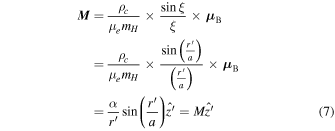
letting

Using Equation (7), the equations for  and
and  become
and at  (the stellar radius)

since  and
and  , which is the upper limit of ξ restricted by the fact that the value of Θ must not become negative because then ρ becomes negative as can be seen from Equation (44) i.e., the boundary of the star is defined by
  . Also, in the above equation
  becomes
  at the boundary of the star. Therefore, Equation (1) becomes

For simplicity, we can evaluate the above equation for a field point along the positive z-axis. Using

and

the magnetic field  can be found as follows:
Here  is the angle between
  and
and  . In the above equation, we have made use of

and

so that the  and
and  components vanish on integrating over
  and we are left with only the z-component of
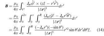
  . Using Equations (9) and (13), we have
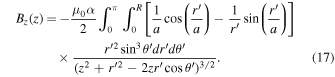
Making use of the table of integrals after letting  in the above equation and then integrating it with respect to the variable μ from the new limits −1 to 1, we get
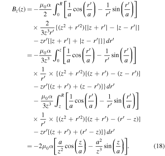
This integral has been split into parts in order to include contributions from all of the source points  and
and  . See Figure 1 for further clarification. Indicated in the diagram are the position vectors of the source and field points:
  and
and  , as well as their difference vector,
  . The integral above has taken into account contributions from all such source point vectors
  , in order to find the magnetic field at an arbitrary field point
  within the star. Because we are, in particular, interested in finding the central B-field; i.e., field at the center of the star, we expand the sine and cosine functions in the above equation into a Taylor series and also neglect terms of higher order for
  to get
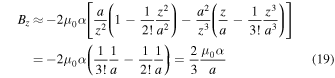
as  . Substituting Equation (8) into Equation (19), we get the central magnetic field Bcen as
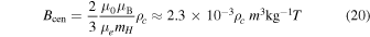
which for central densities in the range  becomes
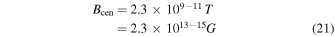
i.e., the lower limit of central magnetic field is of the order of  .
.

Figure 1. Calculation of the magnetic field at an arbitrary point on the z-axis within the star.
Download figure:
Standard image High-resolution image
3. Justification for Such a Spin Alignment inside of the Star
The spin alignment is assumed to have begun when the star was still a main-sequence star. Volume and surface currents would be the source of a magnetic field in such a star. Such a non-zero initial field would start the spin alignment process. When this star collapses to become a degenerate star like a WD, invoking flux conservation, one can justify for the magnetic field amplification (Woltjer 1964).
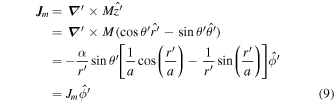
Also, while in a single-degenerate binary star system, such an MWD could accrete mass from its companion star and shrink in size because of increased gravitational contraction (Das & Mukhopadhyay 2013; Das et al. 2013). The magnetic flux could, again, be conserved in this process and become further amplified. This quasi-equilibrium situation of accretion and shrinking continues until the magnetic field exceeds the critical field Bcr and, for some values of the magnetic field as well as Fermi energy, only one Landau level is occupied (Das & Mukhopadhyay 2013; Das et al. 2013). This means that all of the electrons inside of the WD have been aligned in the spin-down state. In the extreme relativistic case, there would then be volume current densities  in the
  -direction, as can be seen from Equation (9). They are responsible for maintaining such a strong field once it has been generated.
A very common source of confusion is the model of an electron gas in an external magnetic field. The interaction energy of a dipole in a magnetic field is  , where B is the local field. B is the field that is present at the location of the dipole if the dipole were to be removed, assuming, of course that this does not affect the surroundings. The presence of this field could be due to an external applied field, as well as due to the presence of the field of the other dipoles in the specimen (Mandl 1988). In our case, the presence of this local field would be due to the magnetization currents, and also the field of the other dipoles that produce the magnetization
  . Thus, we can see that if the equation of state in a magnetic field obeys a relation as given in Equation (38); i.e., for an extremely relativistic situation, we can have central magnetic fields at least of the order of 1013–15G, depending on the density.
4. Summary
In this work, we have given a sample calculation estimating the magnetic field at the center of a magnetic white dwarf star proving that if all of the electrons inside of the star were aligned in the spin-down state by volume current densities, then a very strong central B-field is certainly possible. Although the proof given above is for a simple model and is strictly theoretical, this might also be a possibility in an actual physical star if its equation of state very closely matches  . It is as if the whole star is one giant structure of highly ordered magnetic domains. It would certainly be interesting to see if similar calculations are possible for other equations of state.
We thank the anonymous referee for the invaluable suggestions that helped improve the quality of our manuscript.
Appendix: Equation of State of a One-Landau-level Extremely Relativistic Electron Gas in a Magnetic Field
On solving the relativistic Dirac equation, one obtains the energy eigenvalues of a free electron in an external static and a uniform magnetic field oriented in the z-direction, which are given by Lai & Shapiro (1991):

where  is the Landau quantum number and can take on values
  , which are known as Landau levels. Here,
  is the principal quantum number,
  is the spin quantum number or the spin of the electron, and
  is the dimensionless magnetic field. The critical value of magnetic field Bcr is given by Lai & Shapiro (1991) and Das & Mukhopadhyay (2012) as

Notice that for one Landau level (i.e.,  ) case that has been considered,
  . This means that all of the electrons inside of the star are aligned in the spin-down state. The number density ne of a relativistic electron gas in a volume V in a magnetic field is given by Lai & Shapiro (1991) and Das & Mukhopadhyay (2012) as

where  is the Compton wavelength of an electron,
  is the degeneracy of the Landau level ν such that
  for
for  and
and  for
for  , and
, and  is the unitless Fermi momentum defined by Lai & Shapiro (1991) and Das & Mukhopadhyay (2012) as

where  is the unitless Fermi energy. The upper limit of the summation
  is defined by
where  is the unitless maximum Fermi energy of the system. The matter density ρ is related to the electron number density via

where  is the mean molecular weight per electron and
  is the mass of a hydrogen atom. The electron energy density
  at
at  is
is
where
and the pressure due to such a gas is given by Lai & Shapiro (1991) and Das & Mukhopadhyay (2012) as
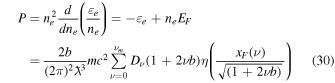
where

Shown below is a simple calculation that gives the equation of state in the extreme relativistic limit (i.e.,  or
or  ) for a one-Landau-level system (i.e., for
  ).
).
The electron energy density  and the electron number density ne, corresponding to
  , can be found from Equations (28), (29), (24), and (25) to be, respectively,
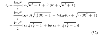
and
where

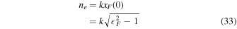
Now, in the extreme relativistic limit, Equations (32) and (33), respectively, become
and

Substituting the above two equations into Equation (30) we get
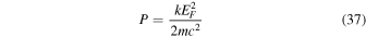
The matter density inside of the WD is given by Equation (27). Therefore, combining Equations (27), (34), (36), and (37) we get
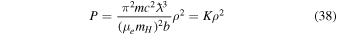
where
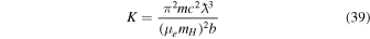
is a constant for a particular value of magnetic field. Pressure and density of a polytropic star can be respectively expressed (Chandrasekhar 1958) as


where K is a constant,  is the central density of the star, Θ is a dimensionless variable, and n is the polytropic index. Comparing Equation (38) with Equation (40) gives us n = 1. The solution of the Lane–Emden equation corresponding to this polytropic index (Chandrasekhar 1958) is given by

where the dimensionless variable ξ is related to the radial distance r by

where a is a scaling factor. Therefore, we have for a n = 1 polytrope
