


Abstract
Planetary obliquity determines the meridional distribution of the annual mean insolation. For obliquity exceeding 55°, the weakest insolation occurs at the equator. Stable partial snow and ice cover on such a planet would be in the form of a belt about the equator rather than polar caps. An analytical model of planetary climate is used to investigate the stability of ice caps and ice belts over the widest possible range of parameters. The model is a non-dimensional diffusive Energy Balance Model, representing insolation, heat transport, and ice−albedo feedback on a spherical planet. A complete analytical solution for any obliquity is given and validated against numerical solutions of a seasonal model in the "deep-water" regime of weak seasonal ice line migration. Multiple equilibria and unstable transitions between climate states (ice-free, Snowball, or ice cap/belt) are found over wide swaths of parameter space, including a "Large Ice-Belt Instability" and "Small Ice-Belt Instability" at high obliquity. The Snowball catastrophe is avoided at weak radiative forcing in two different scenarios: weak albedo feedback and inefficient heat transport (favoring stable partial ice cover), or efficient transport at high obliquity (favoring ice-free conditions). From speculative assumptions about distributions of planetary parameters, three-fourths to four-fifths of all planets with stable partial ice cover should be in the form of Earth-like polar caps.
Export citation and abstract BibTeX RIS
1. Introduction
To first order, surface temperature on Earth decreases from the equator to pole proportionally to the meridional distribution of insolation. The distribution is determined by the solar luminosity, average distance to the Sun, and the axial tilt or obliquity angle β, which is currently 23.45°. Permanent snow and ice cover on Earth (aside from small regions at high elevation) is at present limited to polar caps where insolation is low.
For a planet at high obliquity, this familiar situation would be reversed, because the annual mean insolation (or instellation) at obliquities  is largest at the poles and smallest at the equator. If such a planet were to have stable, permanent partial snow and ice cover, the icy region would be in the form of a belt about the equator rather than polar caps. This arrangement is sketched in Figure 1. We introduce the term "ice belt" to describe this hypothetical climatic state. The sketch also indicates the direction of the meridional heat transport by large-scale fluid motions in the two arrangements: poleward at low obliquity, but equatorward at high obliquity. In both cases, the transport will carry energy across the ice edge from warm to cold regions.

Figure 1. Schematic of annual mean insolation patterns for low and high obliquity, with the corresponding distribution of ice-covered and ice-free regions. We expect ice caps for low obliquity (minimum insolation at the poles) and ice belts for high obliquity (minimum insolation at the equator). Light-red arrows indicate the direction of atmosphere and ocean heat transport. The series expansion of insolation is presented in Section 2.
Download figure:
Standard image High-resolution imageIn this paper, we investigate the conditions under which the ice caps and ice belts sketched in Figure 1 should be expected. We are motivated by ongoing advances in exoplanet observations, which have revealed a wide diversity of planetary sizes, orbits, and host star characteristics. The composition of these planets is still largely unknown and unconstrained. This suggests the use of the simplest possible models of planetary climate to investigate wide ranges of parameters. Our primary goal is to offer some constraints on the planetary characteristics that favor the formation of stable ice belts at high obliquity, and compare these to the more familiar low-obliquity case. Although tidally locked planets may support stable partial ice cover over a wide range of parameter space (Checlair et al. 2017), we limit our study to planets in circular orbits with asynchronous rotation. We make the basic assumption that our hypothetical planet is Earth-like with a N2/H2O/CO2 atmosphere and a surface that is at least partially water covered for habitability (Kasting et al. 1993).
We are interested in investigating the ice−albedo climate feedback in the most generic planetary settings. On Earth, it is well-known that the higher albedo of frozen surfaces relative to unfrozen surfaces introduces a powerful amplifying feedback on externally driven climate changes, and can result in a runaway feedback leading to the so-called Snowball Earth scenario. The degree to which the planetary albedos of ice-free and ice-covered regions differ depends on the spectral energy distribution of a planet's host star, the ice type (water, CO2, etc.), and cloud cover. Water ice is not nearly as reflective of near-IR wavelengths as it is of visible light, such that Joshi & Haberle (2012) argued that ice−albedo feedback for water ice ought to be suppressed on a planet orbiting an M star compared to a G star, like the Sun, all other things being equal. Shields et al. (2013) tested this hypothesis with a hierarchy of models, consisting of a column radiative transfer model, an energy balance model (EBM), and a General Circulation Model (GCM). In all three models, Shields et al. confirmed that ice−albedo feedback was suppressed.
Proposals for ice-belt climatic states go back at least to Williams (1975), who argued that many of the peculiar features of the Neoproterozoic glaciations on Earth (including low-latitude glaciation and apparent strong seasonality) were consistent with high-obliquity insolation. The Neoproterozoic high-obliquity hypothesis has largely been ruled out, both by detailed chronologies and geochemical lines of evidence in support of a "hard Snowball" global glaciation (Pierrehumbert et al. 2011; Hoffman et al. 2017), and by the demonstration that large variations in Earth's obliquity are suppressed by gravitational interactions with our Moon (Laskar et al. 1993; Levrard & Laskar 2003).
This hypothesis, however, did prompt a number of investigations of high-obliquity states with climate models adapted to early Earth conditions (e.g., Hunt 1982; Oglesby & Ogg 1999; Chandler & Sohl 2000; Jenkins 2000, 2001, 2003; Donnadieu et al. 2002). Most of these studies used some form of atmospheric GCM coupled to a shallow mixed-layer ocean and a thermodynamic sea ice model, and thus included representations of the seasonal cycle, dynamical heat transport by the atmosphere, and feedbacks from water vapor and surface albedo. More recent studies of high-obliquity climate have been motivated instead by exoplanet considerations (Williams & Kasting 1997; Williams & Pollard 2003; Spiegel et al. 2009; Abe et al. 2011; Armstrong et al. 2014; Ferreira et al. 2014; Wang et al. 2016).
The studies cited in the above paragraph span a wide diversity of planetary parameters (e.g., solar constant, greenhouse gas amount, continental configuration, obliquity, rotation rate) as well as model realism (e.g., resolution, parameterization of hydrological cycle, ocean heat transport, sea ice physics, land surface model). This diversity makes it difficult to generalize the conditions under which a stable ice belt might occur. However, most of the above-cited studies have investigated ranges of parameters spanning both warm (ice-free) and cold (Snowball) climatic states, and thus might have found an intermediate ice-belt state. Ice-belt climates in models with ice−albedo feedback have been reported by Oglesby & Ogg (1999), Donnadieu et al. (2002), and Abe et al. (2011). Studies that have explicitly looked for ice belts in such models and not found them include Chandler & Sohl (2000), Williams & Pollard (2003), and Ferreira et al. (2014). Jenkins (2000, 2001, 2003) found perennial snow cover on a tropical supercontinent, but did not find any belt-like arrangement of sea ice on tropical oceans. Some of these studies may also be compromised by short integration times; the ice belt may in some cases be a brief transient as the climate drifts toward a fully glaciated Snowball state (e.g., Figure 8 of Jenkins 2003).
There is a long history in the climate literature of studying and quantifying the ice−albedo feedback in simple models of the zonal-average planetary energy budget. Here we present one well-known version of this model, the one-dimensional diffusive EBM (North 1975a, 1975b), and generalize it to the exoplanet context. We subject it to a formal non-dimensional analysis to identify the minimal set of independent parameters. We first examine the seasonal cycle of temperature in a time-varying version of the model. These results offer some insight into the relative roles of local heat storage and heat transport in damping the seasonal temperature range for different obliquities. Limiting our analysis to a regime of weak seasonal amplitudes, we then adopt the more familiar steady annual mean version of the EBM. This model solves for the equilibrium surface temperature distribution in response to the annual mean solar forcing, and offers a generic first-order description ofsome of the important processes on any planet with the possibility of ice−albedo feedback (henceforth just "albedo feedback" for shorthand). There are four parameters, all of which could vary widely in the exoplanet context: radiative forcing (a combined measure of insolation and greenhouse effect), heat transport efficiency, albedo feedback, and the meridional gradient in annual mean insolation. This last parameter is determined entirely by obliquity.
It is well-known that the annual mean EBM has multiple equilibria over parts of its parameter space. For large parts of the parameter space with strong albedo feedback and/or efficient heat transport, we find no stable solutions with an ice edge—only ice free, completely ice covered (Snowball), or both. We show that for high-obliquity planets, stable ice edges are less likely than for low-obliquity planets, in the sense that they exist over a smaller range of the parameter space. In the absence of unforeseen negative feedbacks, multiple equilibria appear to be a robust characteristic of planets with albedo feedback. However, the familiar stable ice edges of Earth may be rarer in high-obliquity worlds.
The rest of our paper is laid out as follows. In Section 2, we present a series approximation for insolation valid at arbitrary obliquity. In Section 3, we introduce the EBM, transform it into non-dimensional form, and explore properties of the seasonal cycle. In Section 4, we present our analytical solutions to the annual mean model with albedo feedback. In Section 5, we use these solutions to investigate the stability of ice caps and ice belts, derive some estimates for the relative likelihoods of observing stable ice edges at different obliquities, and quantify the Snowball bifurcation at low and high obliquity, with implications for planetary habitability. In Section 6, we verify our analytical results against numerical solutions of a seasonal EBM. We conclude in Section 7.
2. Obliquity and Insolation
2.1. Effects of Obliquity on Insolation
Obliquity has a profound effect on the meridional and seasonal distribution of insolation. Figure 2 shows the complete patterns of daily mean insolation for four representative values of obliquity:  (the perpetual equinox),
  (Earth's present-day value),
  (the critical value at which the annual mean equator-to-pole insolation gradient reverses), and
  (the subsolar point is at the North Pole at its summer solstice). In addition to the reversal of the annual mean gradient for
  , the seasonality of insolation is much stronger at high obliquity.

Figure 2. Spatiotemporal distribution of the daily average insolation for four different obliquity values β. Colored contours show the normalized daily average insolation  (unit global, annual mean) with
  , an area-weighted latitude, and
  , a seasonal time angle. For the present-day value
  , we use realistic present-day eccentricity and precessional parameters. For the other three cases (
 ), the eccentricity is set to zero. The thin contours indicate the error of the truncated series fit (2), (3) (contour interval is 0.1, negative contours dashed). The rightmost panel shows the annual mean insolation for the four obliquity values (solid) along with the truncated series fit
  (dashed). These illustrate the reversal of the annual mean insolation gradient at the critical value
  .
.
Download figure:
Standard image High-resolution imageIn the following section, we describe an approximate series expansion for the daily average insolation and show the dependence of the expansion coefficients on the obliquity angle β. We do not treat the diurnal cycle since we use a zonally averaged model.
2.2. Series Expansion of Insolation for Non-eccentric Orbits
In pursuit of a non-dimensional formalism for the planetary albedo feedback problem, we begin by expanding the daily average insolation  in a Fourier–Legendre series (e.g., North & Coakley 1979):


where Q is the global annual average insolation in W m−2 (4Q is known as the solar constant for Earth),  is the normalized daily mean insolation (unit global, annual mean), Pl(x) is the lth-order Legendre polynomial,
  , where tyear is the length of the year, and we use the independent variable
  , where ϕ is the latitude. As shown by North & Coakley (1979), all odd coefficients in this expansion aside from l = 1 vanish. For simplicity we will limit our analysis to circular orbits (zero eccentricity) for which the first harmonic is sufficient when l = 1, and the second harmonic is sufficient for l = 2. Therefore, we truncate the series to

where 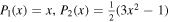 are the first and second Legendre polynomials. Here we are choosing to set t = 0 at the northern hemisphere winter solstice.
For a planet in a circular orbit, s20 (annual mean equator−pole insolation gradient), s11 (amplitude of the annual cycle), and s22 (amplitude of the semiannual cycle) are all simple functions4 of the obliquity angle β:


These coefficients are plotted in Figure 3 for β between 0° and 90°. The distribution of the errors associated with expansion (2) is shown with dashed lines in Figure 2. The rms error of the global annual mean is less than 7% for any obliquity (lower panel of Figure 3). Most of this error lies in the spatial structure of the annual mean at obliquities near zero and in the annual cycle at higher obliquity, so improving this fit would require higher-order Legendre polynomials at low obliquity and higher harmonics of the annual cycle at high obliquity.

Figure 3. Coefficients s20, s11, and s22 of the Fourier–Legendre series expansion of insolation as functions of obliquity β (for planets in circular orbits). The three-term fit captures the pattern with less than 7% rms error (normalized by the global mean insolation) for any obliquity. The dotted line in the bottom panel shows the rms error of the fit 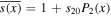 to the annual mean insolation.
Download figure:
Standard image High-resolution imageSince the bulk of this paper focuses on the annual mean energy balance, we note here that the annual mean insolation is

where the overbar denotes an annual average. The coefficient s20 is negative for low, Earth-like obliquity (insolation decreases poleward), reaches zero at the critical obliquity  , and is positive for high obliquity (
 ) for which the poles receive more sunlight annually than the equator. Since β can range between 0° and 90°, s20 ranges between −5/8 and +5/16. We emphasize again that Equation 3(b) is a good approximation for the annual mean insolation for all but very low obliquities (for which s goes to zero at the poles).
3. The Energy Balance Model
3.1. Seasonally Varying Model
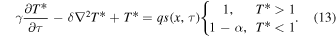
We now adopt the diffusive EBM (North 1975b; North & Coakley 1979), which expresses the zonal mean energy budget for the climate system in terms of the zonal mean surface temperature  . In its seasonally varying form, the model can be written as

where for convenience we define a dimensionless meridional Laplacian operator on the sphere:

The lhs of Equation (5) is the seasonal heat storage, with C a column heat capacity in J m−2 °C−1. The first term on the rhs is the absorbed solar radiation, with a the co-albedo (the absorbed fraction of the incident solar radiation). The insolation function  depends on the obliquity angle β and length of year
  as described in Section 2. A + BT is a linear parameterization of the Outgoing Longwave Radiation (OLR), with dimensional parameters A and B governing its efficiency (dependent on atmospheric properties such as greenhouse gas concentration, cloudiness, lapse rate, etc.). The third term on the rhs represents the convergence of heat transport due to atmospheric and oceanic motions. The transport is parameterized as a diffusive flux down the large-scale temperature gradient, with the diffusivity parameter K setting its efficiency.5
Finally, R is the planetary radius.
as described in Section 2. A + BT is a linear parameterization of the Outgoing Longwave Radiation (OLR), with dimensional parameters A and B governing its efficiency (dependent on atmospheric properties such as greenhouse gas concentration, cloudiness, lapse rate, etc.). The third term on the rhs represents the convergence of heat transport due to atmospheric and oceanic motions. The transport is parameterized as a diffusive flux down the large-scale temperature gradient, with the diffusivity parameter K setting its efficiency.5
Finally, R is the planetary radius.
Albedo feedback is introduced into the model by invoking a temperature dependence of the co-albedo, ![$a=a[T(x,t)]$](https://content.cld.iop.org/journals/0004-637X/846/1/28/revision1/apjaa8306ieqn26.gif) . Following many classic studies (e.g., Budyko 1969; Held & Suarez 1974; North 1975b), we adopt a simple step function in which the ice and snow line is tied to a particular isotherm T0:
. Following many classic studies (e.g., Budyko 1969; Held & Suarez 1974; North 1975b), we adopt a simple step function in which the ice and snow line is tied to a particular isotherm T0:

where  . The temperature dependence of
  introduces a nonlinearity into the EBM and raises the possibility of multiple equilibria and unstable ice growth. For the seasonal model, the natural choice for threshold temperature T0 would be the relevant freezing point (0°C or about
  for Earth's land and ocean surfaces, respectively). Note that the actual freezing point for seawater is salinity dependent and would be lower for a hypersaline ocean (as low as −21.1°C for a NaCl−water brine).
3.2. Annual Mean Model
Many studies using an EBM to analyze features of Earth's climate have focused on annual mean conditions driven by the annual mean insolation  . Averaging the seasonal EBM, Equation (5), over a steady seasonal cycle yields

which is the starting point for many classic studies of Earth's energy balance (e.g., North 1975a, 1975b).
It is often supposed that seasonal covariance between insolation and albedo can be ignored or parameterized. We can define an "effective co-albedo"  for the annual mean energy budget as the ratio

The insolation term in Equation (8) is then replaced with  , with
  given as a function of latitude and obliquity by Equation (4). The annual mean EBM is then closed with an assumption about the dependence of
  on the annual mean temperature
  .
.
Historically, the step-function form of Equation (7) has been applied to the annual mean model, with a threshold temperature Tf typically less than the instantaneous freezing temperature T0. Specifically,

where the canonical choice is  (e.g., North et al. 1981). Why is the relevant threshold −10°C rather than 0°C? This question has received relatively little attention in the EBM literature. The choice of threshold appears to go back to the seminal work of Budyko (1969), who noted that the transition to permanent year-round ice and snow cover in the Arctic occurs at a mean latitude of 72°N, and −10°C is roughly the observed annual mean temperature at this latitude.
Presumably, the transition to permanent ice and snow on a planet with very weak seasonal temperature variations would occur at a location with annual mean temperature closer to 0°C. We thus hypothesize that the magnitude of the difference  is linked to the amplitude of the seasonal cycle. Although preliminary theoretical investigation of this relationship appeared promising, numerical solutions revealed that a step-function parameterization of the co-albedo is unlikely to work when the amplitude of the seasonal cycle is large. We thus defer deeper analysis of Equation (10) to future work. For now, we will simply note that our formal analysis (beginning below) relies on Tf or T0 as a reference point for the non-dimensionalization.
3.3. Non-dimensionalization
For the seasonal model (5), a total of 11 dimensional parameters have been introduced: Q, a0, a1, A, B, K, R, β, T0, tyear, and C. Similarly, the annual model (8) depends on nine parameters—the first eight in the seasonal list, plus Tf (which we hypothesize to be an implicit function of the seasonal parameters). For present-day Earth, many of these parameters are known or can be estimated from observations6
, and  gives a good approximation of the present-day annual mean insolation. Thus, the annual model is often presented as having only one free parameter, the heat diffusion constant K, which is tuned to reproduce the modern-day climate (e.g., North 1975a). However, these parameters can vary widely among exoplanets. It is therefore important to identify all of the key non-dimensional parameters in order to investigate the full range of possible climates embodied in the EBM.
We introduce the following dimensionless constants:


and non-dimensionalize the surface temperature and OLR with

The reference temperature Tref in Equations 11(d) and (12) is taken to be the temperature threshold—either T0 for the seasonal model or Tf for the annual model, so that in either case  at the ice edge.
The seasonal EBM can then be written as
Substituting in the insolation expansion (2) and using Equation (3), we conclude that the seasonal model has five apparently independent parameters:  . These five are usually taken to be uniform in latitude.
The annual EBM can be written as
The annual model has just four independent parameters:  (with s20 uniquely determined by obliquity β). However, the definitions of T* and q are not identical in Equations (13) and (14) because the reference temperatures may differ.
3.4. Physical Interpretation of the Dimensionless Parameters
Here we describe the parameters defined in Equation (11) in physical terms. We provide typical Earth-like values for each parameter and note some factors governing their plausible ranges for habitable exoplanets. The Earth values are derived from dimensional parameters in North (1975b). More accurate or up-to-date values are certainly possible, but our main interest here is in situating the non-dimensional model within the existing EBM literature.
- T*: Proportional to both temperature and OLR.
 by definition at the ice edge.
 - Seasonal heat capacity of the system relative to the radiative decay of temperature over one year. γ decreases with length of year and radiative damping, and increases with fractional ocean coverage and efficiency of ocean mixing. With the dimensional parameters from North (1975b), we have γ ≈ (0.55 m−1)H, where H is the depth of water. for a dry Earth whose heat capacity is dominated by land and atmosphere. A realistic value for Earth is in between 5 and 20, with larger values appropriate for the ocean-dominated southern hemisphere. To apply a uniform gamma requires a compromise across this range.
- Efficiency of dynamical heat transport. δ measures the relative importance of transport versus local radiative damping in response to a localized heat source (Stone 1978). Transport will smooth out meridional temperature variations over length scales smaller than (Lindzen & Farrell 1977). δ depends on atmospheric properties such as mass, greenhouse gas levels and cloud cover, and dynamical factors such as rotation rate and planetary radius (Williams & Kasting 1997; Vallis & Farneti 2009). Other factors might include the topographic forcing of atmospheric stationary waves (e.g., Cook & Held 1988) and the temperature dependence of latent heat transport (e.g., Caballero & Langen 2005). The role of oceans on the effective value of δ is complex due to the multiple spatial scales of ocean heat transport and their tight coupling to the ice extent (e.g., Rose & Marshall 2009; Rose et al. 2013; Ferreira et al. 2014; Rose 2015). Ocean heat transport has been found to increase with rotation rate in uncoupled simulations (Cullum et al. 2014) but decrease in coupled atmosphere−ocean simulations (Vallis & Farneti 2009). For present-day Earth, we take following North (1975b). δ could vary widely across different planets.
- Radiative forcing. The numerator in Equation 11(d) is the global mean absorbed shortwave for an ice-free planet. The denominator is OLR at the ice edge. q is sensitive to solar irradiance (Q), greenhouse gas amount (A), and planetary albedo, as well as choice of reference temperature. q could of course range widely across planets with different orbital distances and stellar output. The region of interest is the habitable zone near , since planets at large or small q would be locked into very warm or Snowball climates, respectively. For Earth, in the annual mean model and 1.1 in the seasonal model.
- A measure of the potential ice−albedo feedback. α is bounded between 0 (no feedback; no change in albedo across the ice edge) and 1 (extreme feedback). α will be reduced for a cloudier planet and vice versa. α is also systematically reduced for cooler host stars with longer emission wavelengths (Shields et al. 2013). For Earth, North (1975b) used values corresponding to .


3.5. Deep and Shallow Limits of the Seasonal Model
Before presenting our analysis of the stability of the annual mean model (14) at high and low obliquity, we take a brief detour into the effects of the seasonal cycle in the time-dependent seasonal EBM. An explicit goal of this analysis is to determine the non-dimensional parameter regime in which the seasonal effects are small, which then justifies the use of the annual mean model.
We begin by removing the nonlinearity from Equation (13) by taking  (uniform, constant albedo). This simplification makes Equation (13) a linear PDE for T*, and allows us to obtain periodic seasonal solutions of the form

where  is the annual mean temperature,
  and
and  are the amplitude and phase lag (relative to insolation) of the annual cycle, and
  and
and  are the same quantities for the semiannual cycle. We non-dimensionalize
  and
and  such that they have zero annual mean.
Solutions for  are discussed later in Section 4.1. In Appendix
which implies that temperature is coherent across latitudes in phase and increases in amplitude linearly with  toward the pole in each hemisphere. The solutions for the semiannual component are
The above solutions show the relative roles for local heat storage and meridional heat transport in the seasonal cycle. Setting  gives a local radiative equilibrium solution in the absence of transport and emphasizes the role of γ in both damping the temperature seasonal amplitude and shifting its phase relative to the insolation.
The deep-water limit is  , appropriate for a planet with a deep mixed ocean layer or short solar year. In this limit, the phase shifts for both annual and semiannual components are nearly
  and the temperature seasonal amplitude is weak. Present-day Earth is much closer to this limit than to the shallow-water limit to be discussed below, as evidenced by the observed phase shift of our seasons. To leading order in
  , the deep-water limits for the annual and semiannual components are


It is notable that the (weak) seasonal amplitude becomes independent of δ in this limit.
Conversely, the shallow-water limit  is appropriate for a dry planet with a very long solar year. In this case, the temperature has large seasonal amplitude nearly in phase with the Sun. Specifically we get, to leading order,


It is notable that even in this limit the seasonal amplitude is substantially smaller than the local radiative equilibrium value ( ) due to transport from other latitudes. Physically, the amplitude of the annual cycle of insolation increases poleward, but this is offset by the poleward increase of the seasonally varying convergence of heat transport from lower latitudes. There is a tradeoff between the damping of the seasonality due to local heat storage versus that due to meridional transport. This damping is stronger for the semiannual than for the annual component, which contributes to the smallness of the semiannual component away from the equator.
In the next section, we will present our analysis of the nonlinear annual mean model with albedo feedback. The annual model is independent of the heat capacity parameter γ, and through Equation (10) assumes a sharp boundary between the ice-covered and ice-free regions. The relevance of these results in the presence of substantial seasonal migration of the snow and ice line is questionable. We therefore limit ourselves to consideration of the deep-water regime  in which those migrations are small, noting that this restriction is more stringent for small, slowly rotating planets (for which δ is larger). We will revisit this question with numerical integrations of a seasonal model in Section 6.
4. Solutions of the Annual Mean Model
We now provide explicit analytical solutions to the non-dimensional annual mean model (14). In what follows, we denote the latitude of the ice edge as xs, i.e.,  .
.
4.1. Ice-free Solutions
Before considering partially ice-covered planets, we first consider solutions with constant albedo across the whole domain. In this case, Equation (14) is linear and simple exact solutions can be written:

for ice-free conditions, and

for Snowball conditions.
An ice-free planet requires the coldest temperature anywhere to be at or above Tf, so  everywhere. The coldest temperature occurs at the pole (x = 1) for low obliquity but at the equator (x = 0) for high obliquity. We define qfree as the minimum radiative forcing for which an ice-free planet can exist. Noting that
  and
and  , the condition is

where we remind the reader that s20 ranges between −5/8 (for  ) and +5/16 (for
  ) (Figure 3).
Notice that this says that ice-free conditions can exist for weaker radiative forcing on high-obliquity planets compared to low-obliquity planets with the same heat transport efficiency, both because  is small (even at extreme
  it is still smaller than for present-day
  ), and because of the extra factor of 1/2 when
  (
( ). Equivalently, warm climates can exist with weaker heat transport efficiency on high-obliquity planets compared to low-obliquity planets at the same radiative forcing. Physically, this arises because the annual mean insolation is larger at the equator for high obliquity than it is at the poles for low obliquity.
As a concrete example, if  for an Earth-like planet, then condition (21) says that an ice-free climate is possible for
  for
for  . Thus, present-day Earth is near a radiative forcing that supports an ice-free climate. On the other hand, for
  , the condition is
  , meaning the planet could support an ice-free climate even under a 10% reduction in insolation (or a similar reduction in global mean temperature from reduced greenhouse gases). Figure 4 shows qfree plotted as a function of β and δ. The smallest radiative forcing for which ice-free conditions are possible occur at values of obliquity close to
  . Here, the annual mean insolation has zero meridional gradient, and
  . Under these conditions, the surface is essentially isothermal and just above the freezing point.

Figure 4. Contour plot of the minimum radiative forcing qfree for which an ice-free solution exists, as a function of obliquity and heat transport efficiency. A logarithmic scale is used for δ since it may vary over orders of magnitudes. For comparison to Earth-like planets, the red contour shows q = 1.2 (the present-day value based on Equation 11(d)), and the Earth symbol (circle with cross) indicates qfree for β = 23.45°, δ = 0.31 from Equation (21). The fact that this point sits on the red line indicates that present-day Earth is near a radiative forcing that supports an ice-free state according to this model.
Download figure:
Standard image High-resolution imageMore generally, Figure 4 shows that qfree is substantially smaller for high obliquity than low obliquity over a wide range of transport parameters δ. All non-dimensional parameters being equal, a high-obliquity planet is more likely to be perennially ice free than a low-obliquity planet.
4.2. Snowball Solutions and Multiple Equilibria
We can similarly define qsnow as the maximum radiative forcing for which a completely ice-covered climate can exist:
It is well-known from EBM studies of Earth's climate that both climatic extremes (ice-free and Snowball) are possible over a wide range of radiative forcings, i.e.,  . The equilibrium climate is multiple valued and capable of undergoing hysteresis, which is central to the Neoproterozoic Snowball Earth hypothesis (e.g., Hoffman et al. 2017). How general is this result? What combination of parameters permits the coexistence of the ice-free and Snowball solutions? From Equations (21) and (22), both solutions are possible for a range of q values as long as the albedo parameter α is sufficiently large—that is, if the planet has a strong enough albedo feedback. Specifically, we can define a minimum value of α that permits both solutions for some range of radiative forcings (whether we are actually in the multiple equilibrium regime would then depend on q). The condition on α is

Or, since  is a small number, to a crude approximation we can write

for either sign of s20. For the Earth-like parameter values cited above, we have  . This condition is then satisfied for any obliquity. We conclude that multiple equilibria are a rather common property of planets with albedo feedback, perhaps especially in the high-obliquity regime since
  is smaller.
4.3. Solutions with Interior Ice Edge
When temperature crosses the ice threshold  somewhere in the domain, Equation (14) becomes nonlinear. However, if we assume that the ice edge xs is known, then the problem is piecewise linear in the warm and icy regions. We can then solve for the parameter values that would give the assumed ice edge. This is the basis for the analytical solutions given by North (1975b) and North et al. (1981). Here we extend these solutions to the high-obliquity case. Details are given in Appendix
Because the icy region exists on opposite sides of xs in the low- and high-obliquity regimes, the appropriate form of the rhs of Equation (14) is slightly different depending on the sign of s20. The upper form applies to  and
and  , or for
  and
and  , while the lower form with the factor
  applies to
  and
and  , or for
  and
and  .
.
These are second-order ODEs (forms of Legendre's equation) for  . Since the annual mean model is symmetric about the equator, we solve on the hemisphere
 ![$x\in [0,1]$](https://content.cld.iop.org/journals/0004-637X/846/1/28/revision1/apjaa8306ieqn103.gif) . We split this domain into two regions
. We split this domain into two regions  ,
,  , and solve a two-point boundary value problem in both regions. The particular solution is proportional to
  following the insolation, and the general solution to the homogeneous equation is written in terms of the Legendre functions on both sides. Four boundary conditions are determined by conservation of energy: zero heat transport at the pole (x = 1) and the equator (x = 0), and continuous transport at xs (which requires that both T* and its derivative are matched at xs). The fifth condition is the ice-edge condition
  , from which we derive a relationship between unknown model parameters valid for a given xs (see Appendix
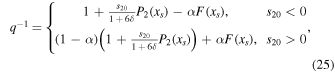
where  is a special function computed in terms of hypergeometric functions, and depends on model parameters δ and
  the formula is given in Equation (43). Equation (25) gives the radiative forcing q required for a given ice edge xs. Although it seems perverse to solve for
  rather than xs(q), the inverse of Equation (25) is multiple valued and does not have a closed form.
5. Caps and Belts: Exploring the Parameter Space
5.1. Stable versus Unstable Ice Edges
The expressions in Equation (25) define the solution space for the EBM. If the planetary properties  , and β (and hence s20) are known, then from Equation (25) we can calculate the radiative forcing q necessary for any ice edge. We might also think of q as known and use Equation (25) to compute the albedo or transport efficiency necessary for a given ice edge. The point is that Equation (25) defines a relationship between the four model parameters for any ice edge xs.
Note that s20 only appears in the solutions (including in the definition of F) as the ratio  . This factor arises because the particular solutions to any forcing term
  in the diffusion Equations (14) are damped by a factor
  diffusion acts to smear out the local forcing, producing a weaker temperature gradient.
In Figure 5, we plot the solutions  for a range of values of δ and α, and for both Earth-like and high obliquity. Because the location of the icy region is reversed at high obliquity (Figure 1), we have reversed the y-axis in the
  plots in the lower row so that up is always cold and toward an ice edge (if it exists). This simplifies the visual interpretation of the stability criterion discussed below. These solutions are multiple valued: there are anywhere from one to five different equilibrium ice edges for any given radiative forcing (which we can visualize by drawing a vertical line through the plot). At most three of these solutions are stable equilibria (and thus physically realizable).

Figure 5. Radiative forcing q required as a function of ice-edge latitude  , for various parameter values. Upper row: Earth-like obliquity
  ice cap is poleward of the indicated latitude. Lower row:
  , warmest temperatures at the poles, ice belt is equatorward of the indicated latitude. The latitude axis is flipped so that the icy region is above the indicated latitude in all cases. Panels (a)–(c) and (e)–(g) show
  computed from Equation (25) for several different values of δ ranging from 0.04 to 2.56. Stable equilibria exist wherever the graphs slope upward to the right. Panels (d) and (h) show the ranges of possible stable ice edges as a function of the albedo feedback parameter α. For a given δ value, stable ice edges are possible only within the shaded region
  .
.
Download figure:
Standard image High-resolution imageThe physical basis of the stability condition is straightforward: the equilibrium size of the icy region should decrease with an increase in radiative forcing, so that small perturbations in the ice extent will excite a net negative radiative feedback and decay. For polar ice caps at low obliquity, the ice edge is stable if

a condition known as the "slope-stability theorem" (Cahalan & North 1979). Locations on the graphs where the slope  changes sign therefore indicate bifurcation points of the ice−climate system. For the familiar low-obliquity case, there are both minimum and maximum sizes for stable polar ice caps (North 1984; Roe & Baker 2010). The associated instabilities have been called the Small Ice-Cap Instability (SICI) and Large Ice-Cap Instability (LICI) or simply Snowball instability.
The green curve in Figure 5(b) is reasonably close to Earth-like parameters (β = 23.5°, δ = 0.32, α = 0.44, q = 1.2) and serves to illustrate the classic Snowball Earth hysteresis. The analogue of the present-day climate sits on the stable ice-cap branch with xs near 60° latitude in this case (though xs is closer to 70° for Earth). A reduction in greenhouse gases or solar constant sufficient to reduce q by about 2% would cause the climate to cool and the ice cap to expand, following the green curve down to the bifurcation point around 38° latitude. A further reduction in q would then trigger unstable ice expansion down to the equator (the horizontal line at the bottom of the graph). Exiting the Snowball scenario would then require sufficient radiative forcing to raise the equatorial surface temperature past the melting point, i.e.,  . From Equation (22), this threshold is about 1.65, or about a 38% increase over the present-day value of 1.2. The planet would then undergo an unstable transition to extremely warm and ice-free conditions (the horizontal line at the top of the graph). Qualitatively, the same statements can be made for any curve in the upper panels that features a stable ice cap over some range of q.
Analogous stability diagrams can be easily computed for any obliquity value. In particular, the perpetual equinox case  is qualitatively similar to the upper row of Figure 5 but somewhat more stable (not shown). However, this result should be treated with caution because of the misfit of the series approximation to
  near the poles for
  (Figures 2 and 3).
For high obliquity, since the ice sits equatorward of xs, the stability condition is reversed. A stable equatorial ice belt requires

Since we have reversed the axes in the high-obliquity plots in Figures 5(e)–(f), the stable solution branches are still readily identifiable in all cases as regions of positive slope. As in the low-obliquity case, there are minimum and maximum sizes for stable ice belts (latitudes at which the slope of the graphs in Figures 5(e)–(f) changes sign). Here we introduce new terminology to describe these bifurcations: the Small Ice-Belt Instability (SIBI) and Large Ice-Belt Instability (LIBI) near the top and bottom of the graphs, respectively.
Stable finite ice cover is far from universal throughout the parameter space at both high and low obliquity. There are, for example, no stable ice edges for very large δ (blue curves); more modest δ admits stable solutions only for small α (weak albedo feedback, e.g., magenta and green curves). Stable ice edges are possible when neither δ nor α is large. In fact, we have already established in Equations (23) and (24) that the product  governs the existence of multiple equilibria due to albedo feedback, and the existence of stable ice edges appears to require that this same product not exceed some threshold. This can also be illustrated through the following approximate stability condition, following Rose (2015).
Suppose that an equilibrated climate is subject to a small globally uniform warming or cooling  , which displaces the ice area by
  . This perturbation is stable if and only if the negative temperature feedback outweighs the positive albedo feedback:

(where the absolute value accounts for the reversed ice orientation at high obliquity). For small perturbations, the ice-edge displacement is determined by the local temperature gradient: 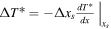 . Taking temperature gradients from the linear solutions (20) then gives

Evaluating this condition near xs = 0.5 (half global ice cover) gives, to a good approximation,

(effectively the opposite of Equation (24)). This is clearly an overly stringent condition because the linear solutions (20) underestimate the temperature gradient near the ice edge, but it serves to illustrate the dependence of stable branches on α and δ. Furthermore, Equation (29) suggests that the condition is more stringent for high obliquity where insolation gradients are weaker, as found in Figure 5.
The exact stability condition can be derived from Equation (25) by setting  and solving for α. Stable ice edges are possible wherever
 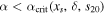 , where the critical value takes on different forms for low and high obliquity:
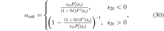
where the primes refer to derivatives with respect to x evaluated at xs.  is shown in Figures 5(d) and (h). Again, as either α or δ increases, the range of latitudes at which stable ice caps or ice belts can be found is reduced.
The model predicts that stable ice edges should be rarer under high obliquity than low obliquity. For example, for Earth-like  but 90° obliquity, stable ice edges occur only for weak heat transport (
 , red curve, and smaller), and these are very sensitive (large ice-edge displacements for small changes in radiative forcing) relative to their corresponding solutions at Earth-like obliquity. For large parts of the parameter space, the only physically realizable solutions are the ice-free and Snowball states, which are plotted as horizontal lines at 0° and 90° in Figure 5.
Finally, Figure 5 also shows that stable ice edges are frequently found in regions of the parameter space in which both ice-free and Snowball solutions are also possible. This is particularly true for the stable ice belts at high obliquity. For example, the red curve in Figure 5(f) has a stable ice-belt branch, but the entire branch coexists with the ice-free and Snowball branches. There are thus no possible transitions from either ice-free or Snowball conditions into this stable ice-belt state involving a hysteresis in q (radiative forcing). In this case, the ice belt is possible but difficult to realize as there is no ready mechanism by which the climate can drift into this state from warmer or colder initial conditions. The abundance of inaccessible ice belts may help explain why ice-belt states have only rarely been found in GCM studies (see our introduction).
5.2. Likelihood of Stable Ice Edges as a Function of Obliquity
As we argued above, the annual mean EBM predicts that stable high-obliquity ice belts should be rarer than stable low-obliquity ice caps. Here we quantify this statement under some simple, speculative assumptions about the probability distributions of planetary parameters. We will evaluate the relative likelihood Lice of finding a stable ice edge as a function of obliquity, where "relative" here means that Lice will be normalized by the probability for the same planetary properties but Earth's current obliquity.
Suppose that we have a known probability distribution of planetary properties

In principle, given δ, α, and q we can calculate the ice edge xs and its stability. Since we have a functional form for  rather than xs(q), we compute probability of a stable ice edge by integrating over all possible ice edges:
where the denominator is equal to unity. By taking the integral in the numerator only over the interval  , we sample just the part of the solution space that contains stable ice edges. We then normalize by the value of Pice at Earth's obliquity:

There is one further complication involving the inaccessible stable solution branches discussed at the end of Section 5.1. We exclude from our probability calculation all states that are inaccessible from either the ice-free or Snowball branch through a hysteresis in q. The method is illustrated in Figure 6. For given values of δ and s20,  (magenta curve) is defined implicitly by the solution of
  . Similarly,
  (cyan curve) is defined implicitly by the solution of
  evaluated at
  . These conditions describe the parameter space boundaries for transitions to the stable ice-edge branch, respectively, from the ice-free and Snowball branches. We then reduce the limit of the integration in Equation (32) from
  to a smaller value
  given by

The maximum value in Equation (34) ensures that we include all stable ice edges that are accessible (through a radiative hysteresis) from at least one side.

Figure 6. Graphical illustration of the method for excluding inaccessible stable states. In color, we contour  from Equation (25) for the stable region bounded by
  from Equation (30). The magenta curve is the implicit solution of
  —the latitude to which the ice edge would jump in an unstable transition from ice-free conditions. The cyan contour is the implicit solution of
  —the analogous ice-edge latitude resulting from unstable transitions from the Snowball state.
  in Equation (34) is the intersection of the magenta curve with
  . For
. For  , transitions from ice-free conditions would result directly in a Snowball. Similarly,
  is the intersection of the cyan curve with
  , giving the maximum α for which transitions from Snowball to stable ice edge are possible. The thick black contour illustrates
  from Equation (34). Inaccessible stable states lie between
  and
and  .
.
Download figure:
Standard image High-resolution imageWe are unable to solve analytically for  (it involves a transcendental equation for xs), but a numerical solution with a root-finding algorithm is straightforward. We thus compute two version of the likelihood Lice: one in which all possible stable ice edges are accounted for using Equation (32), and another in which inaccessible stable states are excluded by replacing
  with
with  in the limits of integration.
Calculating Lice requires a plausible form for the probability distribution hplanet. We assume here that the three parameters  are independent of each other, so that their joint probability distribution is separable:

Alternatively, we might consider some parameter interdependence, e.g., α and δ might co-vary due to the effects of stronger albedo contrasts on atmospheric baroclinicity and eddy activity. We make the separable assumption here for simplicity. Recall that  and
and  are products of several parameters—each of which may vary considerably—and both variables are also positive definite, with no upper bound. These features suggest that taking log-normal distributions for hq and hδ may be reasonable. We lack such a firm basis for the form of hα, but as α is bounded on
 ![$[0,1]$](https://content.cld.iop.org/journals/0004-637X/846/1/28/revision1/apjaa8306ieqn163.gif) , both uniform and beta distributions seem reasonable.
, both uniform and beta distributions seem reasonable.
We adopt three different sets of assumptions, resulting in three different curves in Figure 7. For PDF0 (blue curve), we assume the following: hα is uniform on [0, 1]; hδ is log-normal on ![$[0,\infty ]$](https://content.cld.iop.org/journals/0004-637X/846/1/28/revision1/apjaa8306ieqn164.gif) with shape parameter 1.0, scale parameter 1.0, and location parameter 0 (mode at
with shape parameter 1.0, scale parameter 1.0, and location parameter 0 (mode at  , median at
  ); and hq is log-normal on
 ![$[0,\infty ]$](https://content.cld.iop.org/journals/0004-637X/846/1/28/revision1/apjaa8306ieqn167.gif) with shape parameter 0.5, scale parameter 1.0, and location parameter 0 (mode at q = 0.78, median at q = 1). PDF1 (green curve) is the same as PDF0 except hδ gives more weight to both small and large values of δ (log-normal with shape parameter 2.0 and scale parameter e; mode at
with shape parameter 0.5, scale parameter 1.0, and location parameter 0 (mode at q = 0.78, median at q = 1). PDF1 (green curve) is the same as PDF0 except hδ gives more weight to both small and large values of δ (log-normal with shape parameter 2.0 and scale parameter e; mode at  , median at
  ). Finally, PDF2 (red curve) is the same as PDF1, except hα is a parabolic beta distribution on
 ![$[0,1]$](https://content.cld.iop.org/journals/0004-637X/846/1/28/revision1/apjaa8306ieqn170.gif) with a mode at
with a mode at  , thus giving a higher probability for moderating albedo feedback. In each case, Lice is computed through numerical integration of Equation (32) for a given obliquity value and normalized by its value at Earth obliquity.

Figure 7. Estimates of the relative likelihood Lice of finding a planet with a stable finite ice cover, either ice caps (for low obliquity) or ice belt (for high obliquity). The curves show Lice calculated from Equations (32) and (33) and for three different forms of probability density hplanet as described in the text, and normalized to a value of 1 at Earth's obliquity of 23.45°. Dashed curves include all possible stable ice edges. Solid curves exclude inaccessible stable states using Equation (34).
Download figure:
Standard image High-resolution imageFigure 7 shows that in all cases the likelihood of a stable ice cap decreases with increasing obliquity, approaching zero at the critical obliquity of 55°. The likelihood of a stable ice belt then increases with obliquity between 55° and 90°, but in all cases is lower than the likelihood of a stable ice cap at Earth-like obliquity. The details appear to be most sensitive to assumptions about  (i.e., the red curve is substantially different from the green and blue curves). However, in all cases the shape of Lice is qualitatively similar to the annual mean equator-to-pole insolation gradient
  . As this gradient becomes small near
  , the transport will have an increasingly strong tendency to overwhelm the insolation gradient and produce a nearly isothermal climate either above or below the ice threshold.
At high obliquity, the exclusion of inaccessible stable states has a larger impact on Lice than at low obliquity (as anticipated by the shapes of the  curves in Figure 5). The relative rareness of radiative hysteresis loops that access the stable ice-belt configuration means that such states are less likely to be observed (or modeled). The tentative conclusion (based on these highly speculative assumptions about the distributions of planetary parameters) is that ice belts will be less probable than ice caps, by a factor of 2 or so.
We can go one step further toward a general statement about the observability of ice belts versus ice caps by making an assumption about the distribution of obliquities. If, for example, obliquity is uniformly distributed between 0° and 90°, the area under the curves in Figure 7 on either side of the critical 55° define relative likelihoods of finding stable ice caps versus ice belts. Under this assumption, the proportion of all hypothetically observable stable ice edges comprised of ice belts is then 22%, 24%, or 17% using PDF0, PDF,1 and PDF2, respectively. So, about three-fourths to four-fifths of all planets with partial ice cover would be in the form of Earth-like low-obliquity polar ice caps. Note that these numbers just represent relative likelihoods of ice caps versus ice belts; they do not represent probabilities of finding any of these stable ice-edge states relative to ice-free or Snowball conditions.
Is uniformly distributed obliquity a reasonable prior? Miguel & Brunini (2010) simulated planetary accretion and found a primordial obliquity distribution peaking at 90°. Taking  to fit these results better gives 46%, 48%, or 39% ice belts using PDF0, PDF1, and PDF2, respectively. However, it is not clear that observable obliquities have the same distribution as primordial obliquities, as primordial obliquities can be altered by a variety of mechanisms (e.g., Laskar & Robutel 1993; Correia & Laskar 2001). In particular, high obliquities will be reduced by strong tidal interactions for planets close to their host star, yielding a distribution closer to uniform. Better constraints on obliquity distributions and all planetary parameters are clearly warranted.
5.3. The Snowball Bifurcation at Low and High Obliquity
A question of relevance to life on other planets is whether the Snowball catastrophe occurs at lower radiative forcing at low or high obliquity. There is some conflict in the literature on the role of the Snowball bifurcation in planetary habitability. On the one hand, defining habitability in terms of surface liquid water suggests that a Snowball climate is uninhabitable, which has led various authors to propose metrics of fractional or seasonal habitability for planets with partial ice cover (e.g., Williams & Pollard 2003; Spiegel et al. 2008). On the other hand, not only did photosynthesis persist through Snowball events in Earth' history, but the events may have crucially shaped the subsequent evolution of complex life (e.g., Hoffman & Schrag 2002; Hoffman et al. 2017; Laasko & Schrag 2017). The traditional habitable zone concept assumes a planet with a functioning silicate-weathering feedback and a positive CO2 greenhouse effect (Kasting et al. 1993; Kopparapu et al. 2013). Global glaciation may be triggered on such a planet through a rapid drawdown of atmospheric CO2 that reduces q below the thresholds at which the non-Snowball states disappear. In Earth history, this seems to have occurred through accidents of tectonics (Hoffman et al. 2017). These events are self-terminating through the suppression of silicate weathering and accumulation of a strong CO2 greenhouse. Such transitions can in principle occur anywhere within the habitable zone. Our simple model is unsuited to the tasks of diagnosing the inner edge of habitability (where the relevant physics are the runaway water vapor greenhouse and hydrogen loss to space) or the outer edge (where the relevant physics are CO2 condensation and Rayleigh scattering). However, we can compute the q value at which the bifurcation occurs as a function of obliquity and other model parameters, and whether the transition into the Snowball state occurs from a partially ice-covered state (cap or belt) or directly from the ice-free state.
We therefore define qhab as the smaller of the minimum q necessary for ice-free conditions (given by Equation (21)) and the minimum q for which a stable ice edge exists (if any; a quantity we will call qstab), i.e.,

As discussed above, for large values of δ and α, there are no stable ice edges, so qstab is undefined. Elsewhere it is given implicitly by the solution of  for the critical ice-edge latitude xcrit (the bifurcation point at which
  and the stable branch ends in Figure 5). We evaluate this numerically for given values of
  .
.
Figure 8 shows contour plots of qhab as a function of obliquity and heat transport efficiency δ, for the same three values of α used in Figure 5. These are plotted so that darker colors (red to black) indicate planets that remain Snowball-free under weaker radiative forcing.

Figure 8. Contour plots of qhab, the minimum q required for a non-Snowball climate. qhab, defined by Equation (36), is contoured for the fixed albedo contrast parameter α as a function of obliquity and heat transport efficiency δ. Darker colors indicate smaller qhab, i.e., a planet less prone to the Snowball catastrophe. The black contours indicate values of δ above which  , i.e., the Snowball bifurcation occurs directly from the ice-free state. For δ below this line, the bifurcation occurs from a stable partially ice-covered state.
Download figure:
Standard image High-resolution imageHow does the ice−albedo feedback influence the location and nature of the Snowball bifurcation? Figure 8 illustrates a number of different issues. The Snowball catastrophe is moistly avoided on planets with very weak albedo feedback (small α). Such planets can maintain very narrow bands of open water even when the radiative forcing is weak, and this is nearly equally true for low- and high-obliquity planets. On the other hand, for more than a trivial albedo change across the ice edge, some clear differences emerge between low- and high-obliquity worlds. The differences are best illustrated by the black contours, which show the value of δ above which  . Below this line, the Snowball bifurcation is reached from partial ice cover (ice caps or ice belt). Above this line, the bifurcation is reached from ice-free conditions. Figure 8 shows clearly that this threshold occurs at substantially smaller δ values for high obliquity.
For a concrete example, consider the middle panel of Figure 8 with  . At the Earth-like value of
  , we have
  for
for  , but
, but  for
for  . The high-obliquity planet remains Snowball-free for substantially weaker radiative forcing, and remains entirely ice-free before transitioning to the Snowball for all but very small δ. With any significant albedo feedback, a given planet is less likely to fall into a Snowball state at mid-to-high obliquity than at low obliquity.
In summary, there are essentially two rather different scenarios that favor Snowball avoidance at low radiative forcing: either weak albedo feedback and inefficient heat transport, or efficient heat transport at mid- to high obliquity. The first scenario might be associated with large, rapidly rotating planets orbiting M-dwarfs, where a partially unfrozen region is maintained by relatively weak albedo feedback and inefficient heat transport due to strong zonal flow. The second scenario might be associated with smaller, slowly rotating planets at high obliquity, which would remain completely ice-free even with a potentially strong albedo feedback (large α) from shorter wavelength insolation. Albedo feedback is more likely to drive large climate changes under low obliquity than high obliquity.
We emphasize that these calculations are relevant for planets with oceans anywhere within the habitable zone. Near the outer edge of the habitable zone, a planet with a functioning silicate-weathering feedback should have multiple bars of atmospheric CO2. The resultant strong atmospheric scattering would effectively mask the surface albedo, such that the relevant α value would be small (Wordsworth et al. 2011).
6. Effects of the Seasonal Cycle
The conclusions from Section 5 are based on an annual mean model with a sharp transition between ice-free and ice-covered regions, which we have argued should be valid in the deep-water regime  . It is important to verify (at least approximately) the validity of our analytical results in the presence of a seasonally migrating snow and ice line—particularly since the seasonal cycle is so much more pronounced at high obliquity.
We performed numerical solutions of the seasonal EBM (13) with a seasonally migrating snow and ice line. The seasonal model was forced with full realistic insolation at low and high obliquity rather than the series approximation (2). The seasonal model was implemented and solved numerically using the open-source Python package climlab (Rose et al. 2017). To examine the stability of ice caps and ice belts and generate seasonal analogs of the  curves in Figure 5, we implemented a large parameter sweep designed to find all stable states accessible through a hysteresis in radiative forcing q from either the Snowball or fully ice-free state. We began on the ice-free branch and reduced q by small decrements until the Snowball state was reached. We then increased q by small increments until the model was ice-free again. If any partially ice-covered states were found during either of these sweeps, they were used as initial conditions for additional sweeps to map out the stable branch. The seasonal model was integrated for 600 years for every parameter combination to ensure a steady seasonal cycle. Fractional ice area was then averaged over a single year, and expressed as an equivalent ice-edge latitude (Rose et al. 2013): the latitude of the edge of ice caps or belts assuming interhemispheric and zonal symmetry.
Two versions of this calculation were carried out with differing heat capacities. A "deep-water" case uses  , equivalent to about 90 m of water on Earth. The results are plotted in Figure 9. A more moderate case uses
  or about 9 m of water, and is plotted in Figure 10. In both figures, we reproduce (in dashed curves) the analytical solutions of the annual mean model from Figure 5 for comparison, while the numerical results of the seasonal calculations are plotted as solid dots.

Figure 9. Comparison of ice coverage in the seasonal and annual mean models in the deep-water regime ( ). Dashed lines are the analytical solutions to the annual mean model, identical to Figure 5. Solid dots represent the annual average of the steady seasonal solutions of the seasonal EBM. The seasonal model (13) is forced with real (unapproximated) insolation and integrated numerically out to a steady seasonal cycle before averaging over one year. The dots represent the annual average fractional ice area, expressed as an equivalent ice-edge latitude (Rose et al. 2013). The sets of dots are the result of a comprehensive parameter sweep to find all stable states that are accessible through a hysteresis in radiative forcing q.
Download figure:
Standard image High-resolution image
Figure 10. Same as Figure 9 but for the "intermediate-water depth" regime,  .
.
Download figure:
Standard image High-resolution imageFigure 9 shows that the fit between the seasonal and annual mean models is extremely good in the deep-water limit. In particular, the seasonal model exhibits both SICI and LICI at low obliquity, and LIBI and SIBI at high obliquity, with nearly identical stability thresholds. The exception to this near-perfect fit seems to be that small ice caps are more stable in the seasonal model at weak albedo feedback ( ). At 90° obliquity, the main misfit is the radiative threshold for exiting the Snowball state at the bottom of the graphs, which occurs at somewhat lesser values of q in the seasonal model than the annual model. This figure also illustrates the inaccessibility of many stable ice-belt states as discussed above. Our parameter sweep finds only those solution branches that are accessible from either the ice-free or Snowball state. Taking the lower middle panel with β = 90°, α = 0.44 for example, all stable ice-belt states are excluded except the single branch for
  (weak heat transport efficiency).
The results for  in Figure 10 are completely different. Note that this is an intermediate case between the deep- and shallow-water limits discussed in Section 3.5. At low obliquity, there is good agreement between the seasonal and annual models for the behavior of large ice caps and the LICI thresholds. However, there is no SICI in the seasonal model; instead, there is a gradual and smooth transition to perennially ice-free conditions as the radiative forcing increases. At high obliquity, there is very little quantitative agreement between the annual and seasonal models. In general, the seasonal model predicts substantially more stable ice belts than was found in Figure 5. For moderate α, there is still a well-defined SIBI in the seasonal model but no analogue for the LIBI. Instead, we find a smooth transition from seasonal large ice belts to perennially ice-covered Snowball conditions as the radiative forcing decreases. The annual model predicts an unstable LIBI transition to the Snowball state in all cases, which is not found in the seasonal model.
We conclude that the results based on the annual mean model (Figures 4 through 8) are valid for the deep-water regime in which the seasonal migrations of the snow and ice line are small. The stability of highly seasonal ice caps and ice belts in the intermediate γ regime requires further investigation.
7. Discussion and Conclusion
In this paper, we have invoked one of the simplest models of planetary climate that represents spherical geometry and meridional heat transport to investigate how the surface albedo feedback would manifest itself at different obliquities. In particular, we set out to study the stability properties of partially ice-covered states at high obliquity in which the weakest annual insolation occurs at the equator (which we term the ice belt), and compare these to the more familiar ice-cap states at Earth-like obliquity. Although the diffusive EBM has been studied in numerous previous works, it has not been applied in such a complete and general way to exoplanets. We have expressed the model in non-dimensional form to isolate the fundamental independent parameters, derived a completely general analytical solution for any obliquity (extending classic results from North 1975b), and explored properties of the solution over wide ranges of planetary parameters. In addition to the novel analytical solutions themselves, we have presented a number of new findings based on the EBM solutions, which we briefly summarize below.
The minimum threshold radiative forcing to maintain ice-free conditions is substantially smaller for high obliquity than for low obliquity. Multiple equilibria exist over wide swaths of the parameter space at both high and low obliquity. Stable ice belts are possible but exist over a smaller range of parameters than stable ice caps. Factors that favor the stability of both ice caps and ice belts include weaker albedo contrasts between ice-free and ice-covered regions, weaker efficiency of heat transport, and larger absolute annual mean insolation gradients (i.e., obliquities not close to the critical value near 55°). Many potentially stable high-obliquity ice belts states are inaccessible from any hysteresis in the radiative forcing from either ice-free or Snowball states, and thus less likely to be found.
It is possible to calculate the relative likelihood of finding planets with stable ice belts versus stable ice caps based on probability distributions of planetary parameters. From our tentative but plausible assumptions of these PDFs and uniformly distributed obliquities, we find that stable ice belts are relatively rare. We speculate that about three-quarters to four-fifths of all partially icy planets would be in the form of polar ice caps at low obliquity.
A high-obliquity planet is more resistant to the Snowball catastrophe than a low-obliquity planet, in the sense that a larger reduction of the radiative forcing is required to trigger the transition. The transition is also more likely to occur directly from the ice-free state rather than an intermediate state of a stable partial ice cover.
Unstable transitions between partial ice cover and both ice-free and Snowball climates are possible at both high and low obliquity. We have coined the terms "LIBI" and "SIBI" to describe the transitions from stable ice-belt states to Snowball and ice-free conditions, respectively, in analogy with the "LICI" and "SICI" that have previously been discussed at Earth-like obliquity. The validity of the annual mean model results have been verified against numerical solutions of the seasonal EBM with migrating snow and ice line. The annual mean solutions are very accurate in the deep-water limit of large heat capacity/short solar year, but less so in the intermediate-water depth regime. LICI and SIBI (both transitions involving ice lines at low latitudes) are relatively robust to the inclusion of a seasonal cycle. SICI and LIBI (transitions involving ice lines near the poles) are less robust to seasonality. However, we have demonstrated that SICI and LIBI are still possible in seasonal models in the deep-water regime.
LICI (the traditional Snowball Earth instability) is a fairly straightforward geometrical consequence of the spherical shape of the Earth and the relative flatness of insolation gradients near the equator (e.g., Roe & Baker 2010; Rose 2015). Thus, its robustness to the seasonal cycle is an expected result. The same physical arguments should apply to SIBI at high obliquity, though the more intense seasonality of insolation near the equator (e.g., Figure 2) might play a confounding role. Our seasonal model calculations show that SIBI is in fact robust to the seasonal cycle at 90° obliquity. The more robust bifurcation at high obliquity is between the ice-belt and the ice-free state—not the Snowball.
On the other hand, SICI is more controversial. It is found in the annual mean diffusive EBM, but is not robust to details of the transport parameterization (North 1984), and its existence in more complex models continues to be debated (e.g., Huang & Bowman 1992; Lee & North 1995; Maqueda et al. 1998; Langen & Alexeev 2004; Winton 2008; Rose & Marshall 2009; Ferreira et al. 2011; Wagner & Eisenman 2015). Unlike LICI, the physics of SICI does not readily submit to a geometrical argument. Some have argued that the minimum stable ice-cap size is governed by the diffusive length  (Lindzen & Farrell 1977; North 1984), but this scaling is not obvious from Figure 5 since the stable branch disappears entirely at higher δ. Rather, Figure 5 shows that the minimum ice-cap size increases modestly with both α and δ. The robustness of SICI is relevant here because we have identified an analogous high-obliquity LIBI (unstable transition from partial ice cover to Snowball), which is presumably governed by similar physics.
Wagner & Eisenman (2015) found that SICI is suppressed in a seasonal EBM even in the deep-water regime. This is at odds with our results in Figure 9. The discrepancy seems to stem from differences in model formulation. Their albedo values are equivalent to a smaller α than our "Earth-like" value of 0.44. Figure 9 shows that SICI is suppressed in our seasonal model for small α. Also, their model differs from Equation (5) in the ice-covered domain. They solve a thermodynamic equation for sea ice thickness wherever  . Effectively, the heat capacity C governing the seasonal temperature range is much smaller wherever there is ice in their model. This is an appropriate approximation for zonally symmetric sea ice growing over an ocean mixed layer, but its relevance to generic planets with mixed land and ocean coverage, unknown atmospheric composition, and arbitrary length of year is not clear. Further study of the effects of seasonality and model complexity on SICI and LIBI is warranted. We emphasize again the robust bifurcation at either high or low obliquity involves ice edges at low latitudes rather than high latitudes, and that at high obliquity we expect to find bi-stability and unstable transitions between ice belts and ice-free conditions.
We thank Dorian Abbot for his insightful review that improved the manuscript. We also thank Timothy Merlis and Russell Deitrick for very helpful informal comments. See Rose (2017)7 for the Python code to reproduce all results and figures in this paper using open-source packages. B.E.J.R. was supported by NSF Award AGS-1455071. T.W.C. was supported by NSF Award AGS-1623218. C.M.B. was supported by the National Aeronautics and Space Administration through the NASA Astrobiology Institute under Cooperative Agreement solicitation NNH05ZDA001C.
Appendix A: Linear Seasonal Solutions
Here we provide a few details of the linear seasonal model solutions discussed in Section 3.5. First, plug the periodic solution (15) into (13) and group the  terms to get

Canceling the spatial structure, expanding the cosine and sine terms, and regrouping, we get
The phase shift (16(a)) follows directly from the requirement that the coefficient of  vanish. The amplitude (16(b)) then follows from the identity
  . In dimensional terms, Equation (16) corresponds to a temperature amplitude:

The derivation of the semiannual solution (17) is very similar.
Appendix B: Analytical Ice Edge Solutions
Here we provide details of the derivation of the annual mean ice-edge condition (25). We follow the notation in North (1975b) and extend his solutions to high obliquity. The particular solution to Equation (14) in each region (icy and ice-free) is proportional to  (i.e., proportional to the annual mean insolation). The general solution to the homogeneous equation is given in terms of Legendre functions. The exact solution can be written as
for  (low obliquity), and for
  (high obliquity)
Here, f and P are Legendre functions of non-integer order that satisfy the no-flux boundary condition at the equator and pole, respectively, and C1 and C2 are coefficients chosen to match T* and  at xs. f and P can be computed as hypergeometric functions
  :
:


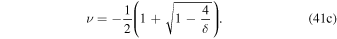
The constants  depend on the ice edge xs:
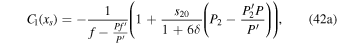
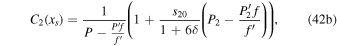
where primes denote derivatives with respect to x, and all terms are evaluated at xs, e.g.,
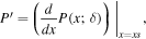
and the derivatives can be evaluated using the identity
Evaluating Equation (40) at  and setting
  gives the relationship (25) between the model parameters for a given ice edge. For convenience we have defined a special function
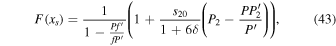
which depends on model parameters δ and  .
.
Footnotes
- 4
- 5
K has units of W
C−1, which is the product of a physical diffusivity in m2 s−1 and a depth-integrated atmospheric heat capacity in J m−2 °C−1. - 6
In principle, A, B, a0, and a1 can all be estimated from satellite measurements of top-of-atmosphere radiative fluxes. However, the complexity of the cloud cover on Earth makes unambiguous determination of these parameters difficult, and estimates in the literature have varied substantially (e.g., Graves et al. 1993; Marani 1999).
- 7
Most recent version: https://github.com/brian-rose/ebm-analytical.
