


ABSTRACT
A self-consistent and spatially dependent model is presented to investigate the multiband emission of pulsar wind nebulae (PWNe). In this model, a spherically symmetric system is assumed and the dynamical evolution of the PWN is included. The processes of convection, diffusion, adiabatic loss, radiative loss, and photon–photon pair production are taken into account in the electron's evolution equation, and the processes of synchrotron radiation, inverse Compton scattering, synchrotron self-absorption, and pair production are included for the photon's evolution equation. Both coupled equations are simultaneously solved. The model is applied to explain observed results of the PWN in MSH 15–52. Our results show that the spectral energy distributions (SEDs) of both electrons and photons are all a function of distance. The observed photon SED of MSH 15–52 can be well reproduced in this model. With the parameters obtained by fitting the observed SED, the spatial variations of photon index and surface brightness observed in the X-ray band can also be well reproduced. Moreover, it can be derived that the present-day diffusion coefficient of MSH 15–52 at the termination shock is  , the spatial average has a value of
  , and the present-day magnetic field at the termination shock has a value of
  and the spatial averaged magnetic field is
  . The spatial changes of the spectral index and surface brightness at different bands are predicted.
Export citation and abstract BibTeX RIS
1. INTRODUCTION
Pulsar wind nebulae (PWNe) are generally believed to be the very high energy γ-ray sources, which are created by the interaction of the pulsar wind with the nonrelativistic ejecta of the ambient supernova remnant (SNR; Goldreich & Julian 1969; Kennel & Coroniti 1984a). A termination shock is formed in the interaction and then the particles are accelerated to extreme relativistic energy at the shock (Rees & Gunn 1974; Kennel & Coroniti 1984b). From the termination shock, the high energy particles are injected into the nebula, and emit photons ranging from radio to TeV γ-rays during the evolution of the PWN. In recent years, the High Energy Stereoscopic System (H.E.S.S.) survey of the galactic plane has detected about 30 PWNe as the γ-ray sources (see a recent status report of Carrigan et al. 2013), which probably provided more information to study the radiation processes of PWNe.
To explain the multiband spectral energy distribution (SED) of a PWN, various models have been proposed. Usually, the radio and X-rays are attributed to the process of relativistic electron's synchrotron radiation, and the very high energy γ-rays are produced by the inverse Compton scattering with various soft photons (Atoyan & Aharonian 1996; Gaensler & Slane 2006). In addition, the relativistic particles coming directly from the pulsar magnetosphere are usually assumed to be uniform (e.g., Zhang et al. 2008; Fang & Zhang 2010; Tanaka & Takahara 2010; Martín et al. 2012; Zhu et al. 2015). In their models, the distribution of particles is spatially independent and the diffusion of particles is often approximated as an escape timescale or neglected. In this case, the multiband observational results of a PWN can be well reproduced by these models. However, the observations implied that the photon index in the X-ray band is a function of position (e.g., Slane et al. 2000; Bocchino et al. 2001, 2005; Mangano et al. 2005; Schöck et al. 2010; Holler et al. 2012). Moreover, Tang & Chevalier (2012) used a model with diffusion to study the spectral index profiles of Crab, 3C 58, and G21.5-0.9, and found that the advection-diffusion model can fit the spectral index profiles better than the pure advection model, which means that the diffusion probably plays an important role in changing the particle spectral index. Vorster & Moraal (2013) calculated the particle (e.g., electron) spectrum as a function of distance by solving the Fokker–Planck transport equation, and studied the effect of diffusion on the particle spectrum in PWN. In their calculations, the spatial distributions of magnetic field and convection velocity in PWNe are approximated as  and
and  , respectively, which are qualitatively similar to the results calculated by Kennel & Coroniti (1984a), but will break down in the case of
  . They expected that particle diffusion is important for reducing the amount of synchrotron losses, and then explained the variation in the photon index of the X-ray synchrotron radiation as a function of position. Recently, Porth et al. (2016) investigated the particle diffusion in PWNe using three-dimensional magnetohydrodynamic (MHD) simulations. In their model, an eddy particle diffusion is adopted, and the distributions of the magnetic field and the convection velocity in the PWN are described as the Gaussian functions, respectively, which are derived from fitting the averaged data predicted by the MHD model, and then these Gaussian functions can easily be incorporated into the kinetic equation. In the steady-state system, for simplicity, this model under the assumption of spherical symmetry (i.e., diffusion coefficient only has radial component) can well reproduce the spatial variation in the photon index of X-ray synchrotron emissions of G21.5-0.9, Vela, and 3C 58. However, in this model, an adiabatic heating effect will appear in the inner regions of the PWN due to the effect of the rapid decrease in velocity in these regions (Porth et al. 2016).
Motivated by the above discussions, we describe a self-consistent and spatially dependent model to study the multiband emission of PWNe. In this model, the magnetic field in the PWN is assumed to be toroidal and the spatial variations of magnetic field and convection velocity are described by the semi-analytic model of Kennel & Coroniti (1984a); the dynamical evolution of the PWN is described by using the model of Bucciantini et al. (2011); the temporal evolutions of electron and photon spectra are self-consistently solved in this system. In our treatment, the temporal spectral evolution of electrons is described as a Fokker–Planck equation in spherical coordinates, where the electrons are injected with a time-dependent broken power law (e.g., Atoyan & Aharonian 1996; Venter & de Jager 2006), and the processes of convection, diffusion, and adiabatic and synchrotron radiation losses (Vorster & Moraal 2013), as well as inverse Compton scattering loss and photon–photon pair production are included; meanwhile, the temporal spectral evolution of photons is described as a spatially dependent conservation equation. This model is applied to MSH 15–52 to explain the multiband observed data and the spatial variations of photon index and surface brightness in radio, X-ray, and γ-ray bands.
The paper is organized as follows. In Section 2, we describe the self-consistent spatial model and numerical method. In Section 3, we apply the model to the MSH 15–52. Finally, in Section 4, we give the conclusions and discussions.
2. THE MODEL
A realistic PWN is a dynamical system that has significantly and complicatedly expanded (e.g., Chevalier & Fransson 1992; Blondin et al. 2001; Van der Swaluw et al. 2001; Gelfand et al. 2009; Bucciantini et al. 2011) and has a quite complicated magnetic field structure shown in MHD simulations (e.g., Del Zanna et al. 2004; Porth et al. 2014). In the self-consistent and spatially dependent model, for simplicity, under the assumption that the system is spherically symmetric and the magnetic field in the PWN is toroidal, the dynamical evolution of the PWN is simulated using the model of Bucciantini et al. (2011) and the spatial variations of magnetic field and convection velocity are calculated with the semi-analytic model of Kennel & Coroniti (1984a). The self-consistent and spherical symmetric model can only apply to the young PWN before the reverse shock crushes the nebula, because the structure of the nebula could be very complicated after the crushing phase and a bow shock nebula could possibly form due to asymmetric compression in this phase (e.g., Chevalier 1998; van der Swaluw et al. 1998, 2004). In such a system, a central pulsar has a spin-down luminosity L(t), which is given by (Pacini & Salvati 1973)
where L0 is the initial spin-down power, n is the breaking index, and  is the initial spin-down timescale of the pulsar, which is determined by the current pulsar period P, its time derivative
  , age of the pulsar
  , and pulsar moment of inertia I (e.g., Gaensler & Slane 2006; Slane 2008). It is believed that a major fraction of the spin-down luminosity of a central pulsar will be converted into the mechanical luminosity of a pulsar wind. Relativistic electrons of such a wind will propagate through a surrounding medium and be accelerated at the termination shock of the pulsar wind, and then injected into the PWN (Kennel & Coroniti 1984a; Aharonian et al. 1997). Meanwhile, non-thermal photons are produced through various mechanisms of the relativistic electrons. Below, we describe the evolutions of relativistic electrons and non-thermal photons in the system and our numerical method.
2.1. Basic Equations
On the one hand, the electron's evolution is generally described as the Fokker–Planck equation (e.g., Parker 1965), but in the spherically symmetric system, the equation can be simplified (e.g., Vorster & Moraal 2013). On the other hand, non-thermal photons' evolution can be described by the photon conservation equation (Mastichiadis & Kirk 1995). Assuming the number density of the electrons with Lorentz factor γ is  (i.e., the number of particles in the energy interval (
 ) at time t and radial distance r per unit volume), and the photon's number density is
  with the dimensionless photon energy
  , we can express them as
and

respectively. The physical quantities in Equations (2) and (3) are described as follows.
In Equation (2), the momentum diffusion in spherical coordinates is neglected,  is the sum of energy losses and is given by

where  is the adiabatic loss, which is

where V is the convection velocity;  is the synchrotron loss and is given by (Rybicki & Lightman 1979)

where  is the Thomson cross-section and
  is the magnetic field energy density;
  is the IC loss and is given by (Blumenthal & Gould 1970)
where xi and xf are the initial and final energies of the scattered photons, respectively, H is the Heaviside step function and  is the distribution of target photon fields,
  ,
,  , and
, and 
 .
.
In the above expressions of Equations (4)–(7), the electron's energy losses depend on the PWN evolution. As mentioned above, we calculate the dynamical evolution of the PWN using the model of Bucciantini et al. (2011). In their model, the dynamical evolution of a PWN is divided into three phases: initial free-expansion, reverberation, and Sedov–Taylor phases. The object is assumed to be a spherical symmetry and the proper motion of the pulsar is neglected and the radiation losses of the particles are negligible. For the young objects, such as Crab, 3C 58, and MSH 15–52, dynamic modeling indicated that they are expanding in the free-expansion phase (Bucciantini et al. 2011). In this case, combined mass and momentum conservation with the energy conservation, an analytic solution with a series expansion is derived to calculate the radius of the PWN in the free-expansion phase
where  is the energy of the supernova explosion,
  is the mass of supernova ejecta,
  , and the expressions of the coefficients ci are shown in Bucciantini et al. (2004). Moreover, the radius of the termination shock can be estimated as

where  is the pressure of the gas at the termination shock (see Equations (7) and (18) of Bucciantini et al. 2004).
Assuming that V0 is the convection velocity at r0, the convection velocity at any radius r, which depends on the magnetization parameter σ and decreases with the increase of radial radius, can be written as

where v(r) is the radial profile of the velocity and it is a dimensionless quantity (see Equations (4.11) and (5.12c) of Kennel & Coroniti 1984a). Following Kennel & Coroniti (1984a), the convection velocity at the termination shock is given by
Based on the MHD restrictions shown in Kennel & Coroniti (1984a), i.e.,  , where B0 is the magnetic field strength at r0 and is determined by the spin-down power L(t), so the temporal evolution of the radial magnetic field can be expressed as

where  is calculated by
  where
where  is the magnetic energy. In an expanding system, the magnetic energy is balanced by the injection rate of electromagnetic energy and the adiabatic loss. Thus, the magnetic energy can be obtained by the equation (Torres et al. 2013)

where  is the magnetic energy fraction and
  is the rate of electromagnetic energy (e.g., Gelfand et al. 2009). Thus, the magnetization parameter can be expressed as
  .
.
Once the radial magnetic field is determined, we can estimate the diffusion coefficient κ, which can be written as  , where
  is the diffusion coefficient at r0 (Lerche & Schlickeiser 1981; Caballero-Lopez et al. 2004). Following Caballero-Lopez et al. (2004), the radial dependence of diffusion
  can be modeled as
  and the energy dependence of diffusion
  is given by
  . Therefore, the diffusion coefficient is given by

In Equation (2), there are two injection terms of the electrons, one represents the electrons derived from the central pulsar, which are accelerated at the termination shock of the pulsar wind and then injected into the PWN (Kennel & Coroniti 1984a; Aharonian et al. 1997), the other represents the injection of electrons produced in the photon–photon pair production process. For the first injection term, the multiband observations of photon emissions from the PWN indicated that the electron spectrum can be divided into two components (e.g., Weiler & Panagia 1978; Gaensler & Slane 2006). Therefore, the particle evolution models often use a broken power law to describe the spectrum of the injected relativistic electrons (e.g., Venter & de Jager 2006; Zhang et al. 2008; Tanaka & Takahara 2010; Martín et al. 2012; Zhu et al. 2015), and then the injection rate is assumed to be

where  is the break energy and the parameters
  and
and  are the spectral indices.
  is the normalization coefficient and is estimated by

The second injection term is given by (Coppi & Blandford 1990)
where

with  and H is the usual Heaviside function.
We now turn to Equation (3),  is the photon escape timescale. In the right side of Equation (3),
  is the emissivity of the synchrotron radiation and is given by (Blumenthal & Gould 1970)

where  is the single particle synchrotron emissivity

where  ,
,  with
with  , and
, and  is a modified Bessel function of the order of 5/3.
  is the emissivity of IC scattering in the Klein–Nishina regime and is given by (Blumenthal & Gould 1970)

where  is the scattered photon emissivity per electron
where xi is the energy of target photons, and x is the final energy of photons, the soft photons in IC scattering include the cosmic microwave background (CMB), the galactic far-infrared background (FIR), the near-infrared and optical photon field due to the stars (NIR), and synchrotron photons. The exact value of each photon field will be defined in Section 3.  is the loss term for the photons due to synchrotron self-absorption and can be written as (Rybicki & Lightman 1979; Mastichiadis & Kirk 1995)
where  is the fine-structure constant, and
  with
with  is the critical magnetic field. Finally,
  is another loss term of the photons due to photon–photon pair production, and is expressed as (Coppi & Blandford 1990)
2.2. The Numerical Method
To solve the particle spectrum evolution in Equation (2), an Alternating Direction Implicit method (Douglas 1962) is used and the boundary conditions of both energy and radius must be determined. In the energy direction, following Vorster & Moraal (2013), the free-escape boundary conditions are imposed, i.e.,  and
and  . The Larmor radius
  of the particles must be smaller than the termination shock radius, which leads to the maximum energy of electron satisfying

where ζ is the compression ratio at the shock, and for strong shocks ( ),
),  (Venter & de Jager 2006). The parameter ε is the shock radius fraction and is defined as
  . In the radial direction, the particles in the outer boundary should escape from the system. Thus, the outer boundary condition is given by
  . In the inner boundary, which is located at the termination shock, the number of the particles should be equal to the injected particles. Thus, the inner boundary condition can be written as (e.g., Ng & Gleeson 1975)

Equation (3) is numerically solved using the Crank–Nicolson method (Crank & Nicotson 1996) and the free-escape boundary conditions are also imposed, i.e.,  and
and  . The spatial average radiation luminosity at different positions can be calculated by

where  and
and  is the photon energy. The surface brightness at different positions are calculated according to Holler et al. (2012).
3. APPLICATION TO MSH 15–52
In this section, we apply the model to MSH 15–52 (G320.4-1.2 or HESS 1514-591). This PWN is a composite SNR that is associated with the energetic pulsar PSR B1509-58 (or PSR J1513-5908). The pulsar has a 150 ms rotation period (Seward & Harden 1982; Trussoni et al. 1996). As one of the the youngest and most energetic known in the galaxy, it has a period derivative of  , a characteristic age of ∼1600 years, and a measured braking index
  (Livingstone et al. 2005). Based on the HI absorption measurement, the value of the distance to system is estimated to be 5.2 ± 1.4 kpc (Gaensler et al. 1999), and the age of MSH 15–52 is likely lower than ∼1700 years from the observation of HI emission (Dubner et al. 2002).
In the radio band, Gaensler et al. (2002) estimated that the flux density at both 0.8 and 1.4 GHz is 2 ± 1 Jy based on the data from Whiteoak & Green (1996) and Gaensler et al. (1999). In the X-ray band, the observations of the Chandra satellite have revealed that the PWN has a power-law photon index of 2.05 ± 0.04 in the energy band of  (Gaensler et al. 2002). At hard X-ray energies, the PWN has been observed with BeppoSAX and INTEGRAL-IBIS telescopes. The power-law fit of the emission from the PWN gave a photon index of 2.1 ± 0.2 and a flux of
  in the 20–200 keV energy range (Mineo et al. 2001; Forot et al. 2006). In the GeV γ-ray band, the PWN was detected by the Fermi-LAT, and the LAT spectrum can be well described by a power law with a photon index of
  in the 1–100 GeV energy band (Abdo et al. 2010). In the very high energy γ-ray band, the PWN was measured by H.E.S.S., and the energy spectrum can be well fitted by a power law with a spectral index of
  in the energy range of 280 GeV to 40 TeV (Aharonian et al. 2005).
The observations revealed that MSH 15–52 has two outflow jets in the southeast and northwest directions and has a large thermal shell structure (RCW 89) in the north of the PWN, especially bright and extended in X-rays (Gaensler et al. 2002; Yatsu et al. 2005; Forot et al. 2006; Yatsu et al. 2009; An et al. 2014). At very high energies, the source also shows a similar morphology as that shown in X-rays (Aharonian et al. 2005; Nakamori et al. 2008). These observations show that the geometric structure of MSH 15–52 is very complicated and deviates from the spherical symmetry. As the first-order approximation, we apply the self-consistent and spherical symmetry model to MSH 15–52, which can help us to study the effects of radial variation of azimuthally integrated spectra in the PWN.
In our calculation, we used the parameters show in Table 1. The initial sin-down timescale  is determined by the observations (e.g., Gaensler & Slane 2006). With an age of
  and an initial spin-down power of
  , the current spin-down luminosity of the pulsar is
  , which is consistent with the value derived from Livingstone et al. (2005) due to the uncertainty of the moment of inertia. The SN explosion energy of
  is higher than that shown in Torres et al. (2014) and Fang & Zhang (2010) because the radius of the PWN in our model is larger. However, our modeling result
  is consistent with the observed results of
  (e.g., Gaensler et al. 2002; Schöck et al. 2010; An et al. 2014). Moreover, the SN explosion energy is consistent with the value of
  adopted by Bucciantini et al. (2011). The soft photon fields in the calculation are the same as that adopted in Torres et al. (2014), i.e., the
  CMB has an energy density of
  , the
, the  FIR has a energy density of
  , and the
  NIR has a energy density of
  .
.
Table 1. Values of Parameters for MSH 15–52
| Input Parameters | Symbol | Value |
|---|---|---|
Ejected mass ( ) ) |

|
4.0 |
SN explosion energy ( ) ) |

|
15.0 |
Period ( ) ) |
P | 150 |
Period derivative ( ) ) |

|

|
Initial spin-down power ( ) ) |
L0 |

|
| Initial spin-down timescale (years) |

|
290 |
| Braking index | n | 2.839 |
| Age (years) |

|
1450 |
| Distance (kpc) | d | 5.2 |
| Shock radius fraction | ε | 0.4 |
| Fitted Parameters | ||
| Magnetic fraction | η | 0.04 |
| Low energy power-law index |

|
1.65 |
| High energy power-law index |

|
2.45 |
| Break energy |

|

|
Initial diffusion coefficient( ) ) |

|

|
Download table as: ASCIITypeset image
We now study the variations of both electron and photon spectra with radial distance. We calculate the present-day electron spectra and the corresponding non-thermal photon spectra at different positions, and the results are shown in Figure 1. The results indicate that both electron and photon spectra of the PWN are all a function of distance and decrease with increasing the distance. The spectrum shift to lower energies is attributed to adiabatic losses and the spatial variation of the spectral shape is dominated by the magnetic field and diffusion coefficient (e.g., Vorster & Moraal 2013; Lu et al. 2016).

Figure 1. Present-day electron spectra (upper panel) and the corresponding non-thermal photon spectra (bottom panel) of MSH 15–52 at different positions. From top to bottom, red line at  , green line at
  , blue line at
  , magenta line at
  , olive line at
  , and black line at
  ;
;  is the dimensionless energy of photons.
Download figure:
Standard image High-resolution imageAs mentioned in Section 2, non-thermal photons are produced by various radiation mechanisms. So it is worth investigating the different photon components with the distance. As an example, Figure 2 shows the spectra of non-thermal photons at different positions of  and
and  , respectively. It is obvious that the radio and X-rays emission from the PWN are produced by the synchrotron radiation and γ-rays are mainly produced via the inverse Compton scattering with the FIR and NIR photons. Moreover, FIR and NIR are the major contributors to the high energy spectra of MSH 15–52 at all of the positions, while the contribution of self-synchrotron Compton (SSC) becomes less and less important as the distance increases.

Figure 2. Different components of non-thermal photons of MSH 15–52 (synchrotron emission (red line), inverse Compton scattering with the CMB (blue line), FIR (magenta line), NIR (black line), and synchrotron photons (green line)) at different positions of  (upper panel) and
  (bottom panel),
  is the dimensionless energy of photons.
Download figure:
Standard image High-resolution imageIn order to study the effect of photon–photon pair production on the SED and the spatial photon index distribution of MSH 15–52, we calculate the present-day timescales of the photon escape and the photon–photon pair production changing with the photon energy, respectively, and the results are shown in Figure 3, where the photon escape timescale is calculated by  and the photon–photon pair production timescale is given by

Compared to the photon escape, the process of photon–photon pair production is negligible because of the timescale of  in all of the positions. Therefore, the process of photon–photon pair production has little effect on the SED and the spatial photon index distribution of MSH 15–52. In fact, the photon–photon pair production process can affect the photon spectrum only when some specific conditions are satisfied (more details are shown in Petropoulou & Mastichiadis 2011).
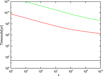
Figure 3. Present-day timescales of photon escape (black line) and photon–photon pair production at different distances of r = 28.1 arcsec (red line) and r = 279.9 arcsec (green line).  is the dimensionless energy of photons.
Download figure:
Standard image High-resolution imageWe also calculate the distributions of the surface brightness at different positions of the PWN in MSH 15–52 and the results are shown in Figure 4, where the different color lines correspond to the surface brightness at different positions. It is clear that the surface brightness of the PWN is also a function of distance. Especially in the X-rays, the photon index strongly depends on distance because the electron spectral index in the high energy varies with the distance (see Figure 1).

Figure 4. Distributions of the surface brightness of the PWN in MSH 15–52. The different colored lines correspond to the surface brightness at different positions and E is the energy of photons.
Download figure:
Standard image High-resolution imageWe use our model to fit the observed SED of MSH 15–52 and the result is shown in Figure 5. The  value of the model results with the observed data is 2.86. Note that an upper limit arrow presented around 0.1 MeV, which is obtained from Forot et al. (2006) based on the INTEGRAL-IBIS telescopes, implies a sharp declining in the energy range. Forot et al. (2006) pointed out that the possible spectral break near 160 keV can be explained by a simple jet scenario with efficient synchrotron cooling, and it is beyond the discussion in our paper. From the model, a present-day magnetic field
  at the termination shock is derived. The value of the magnetic fraction
  , i.e., the magnetization parameter
  , implies that the PWN in MSH 15–52 has a strong shock. This also means that the convection velocity has a value of
  at the shock. For a strong shock with
  , a present-day spatial average magnetic field of
  is derived. This result is slightly smaller than the value of
  obtained by Aharonian et al. (2005). With an initial diffusion coefficient of
  , the present-day diffusion coefficient at the shock is estimated to be
  and a spatial average diffusion coefficient
  of the PWN is obtained, which is smaller than the value that was estimated by An et al. (2014) using the advection-diffusion model shown in Tang & Chevalier (2012), i.e., the diffusion coefficient is estimated to be
  for the magnetic field strength
  . It should be pointed out that the fitting around
  is not very good, which may be caused by using the same soft photon fields as those of Torres et al. (2014) in this paper. We believe that choosing different densities and temperatures of the soft photon fields can get a good fitting.

Figure 5. Spectral fitting result of MSH 15–52. The observational dates are obtained from Gaensler et al. (1999, 2002) for the radio band; Mineo et al. (2001) and Forot et al. (2006) for the X-rays; Aharonian et al. (2005) and Abdo et al. (2010) for the γ-rays.
Download figure:
Standard image High-resolution imageUsing the parameters obtained by fitting the observed SED, we calculate the variations of the spectral index and surface brightness with the distance for the PWN. Schöck et al. (2010) integrated the spectrum over the full azimuthal angle and analyzed the changes of the spectral index and surface brightness in the energy range of  by using the XMM-Newton data under the assumption of spherical symmetry. Their results clearly showed that the photon index increasing with the increase of distance while the surface brightness decreases as the distance increases in the X-ray band. An et al. (2014) studied the radial variation of the photon index and surface brightness in the energy range of
  based on the NuSTAR data. Different from Schöck et al. (2010), they analyzed the northern nebula and the jet separately because the spectral index has a significant variation in the azimuthal direction. Their results also showed that the photon index increases but the surface brightness decreases with the distance in X-rays in the northern nebula. The comparisons of our results with the observed data in the energy range of
  given by Schöck et al. (2010) and in the energy range of
  obtained from An et al. (2014) are shown in Figure 6. It is clear that the radial variations of the photon index and surface brightness in X-rays detected by the XMM-Newton and the radial variation of the photon index in X-rays in the northern nebula observed by NuSTAR can be reproduced in the frame of our model. However, the radial variation of the surface brightness in X-rays in the northern nebula detected by the NuSTAR cannot be reproduced well in our model. A possible reason may be that the radial surface brightness data obtained from An et al. (2014) only include the annular regions in the northern nebula and the southern part is neglected, while we just consider the case that the spectrum is integrated over the full azimuthal angle.

Figure 6. Variations of the photon index (upper panel) and surface brightness (bottom panel) of MSH 15–52. The XMM-Newton data in the energy range of  are obtained from Schöck et al. (2010), and the NuSTAR data in the energy range of
  are obtained from An et al. (2014).
Download figure:
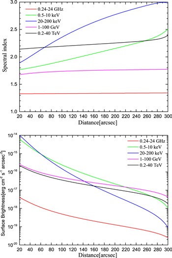
Standard image High-resolution imageFinally, we predict the changes of the spectral index and surface brightness with the distance in the radio, X-ray, and γ-ray bands. Our calculating results are shown in Figure 7, where the above parameters are used. It can be seen that the spectral indexes depend on the distance in almost all of the energy ranges except in the radio band. Especially, in the energy ranges of  and
and  , the spectral indexes have an obvious increase with the increase of distance. While in the energy of
  , the spectral index only slightly varies as the distance increases. In the energy range of
  , the variation of spectral index also is not very obvious, except in the region close to the outer boundary of the PWN. Although the spectral indexes in these energy ranges all increase with the increase of distance, the changing characteristics are not identical (see Figure 7). Note that the variation of the spectral index in the TeV γ-rays is not consistent with that predicted by Schöck et al. (2010), because their radially symmetric model does not include the effect of particle diffusion and the dynamical evolution of the PWN. The results also show that the surface brightness of MSH 15–52 decreases with the increase of distance in all of the energy ranges, but the spatial changing characteristics are also not identical. Especially, the surface brightness has more obvious change in X-ray band (see Figure 7).
Figure 7. Variations of the spectral index (upper panel) and surface brightness (bottom panel) of the PWN in MSH 15–52. The different colored lines correspond to the photon index in the different energy ranges.
Download figure:
Standard image High-resolution image
4. SUMMARY AND DISCUSSION
In this paper, a self-consistent and spatially dependent model is presented to study the multiband emissions of PWNe. In the model, the temporal evolution of electrons is described as a Fokker–Planck equation and the processes of convection, diffusion, adiabatic loss, radiation loss, and photon–photon pair production are included. The temporal evolution of non-thermal photons is given by a spatially kinetic equation with the processes of synchrotron radiation, inverse Compton scattering off soft photons, synchrotron self-absorption, and the pair production including. Numerically solving these two equations, we studied the spatial variations of electron spectrum and multiband radiative properties of the PWN in MSH 15–52 with appropriate parameters.
In the modeling of the SED of a PWN, it is usually assumed that the particles in the system are uniform and isotropic. However, the observations implied that the photon index in the X-ray band is a function of position (e.g., Slane et al. 2000; Bocchino et al. 2001; Mangano et al. 2005; Schöck et al. 2010; Holler et al. 2012). Furthermore, Vorster & Moraal (2013) and Tang & Chevalier (2012) pointed out that the diffusion of particles plays an important role in changing the particle spectral index. In our calculations, we found that the SEDs of both electrons and non-thermal photons are all a function of distance (see Figure 1). We note that the photon indexes in the X-ray band have a more obvious increase with the increase of distance (see Figure 7). The main reason is that the spatial variation of electron SED in the higher energy part is dominated by the competition between synchrotron loss and diffusion (Lu et al. 2016), so the photon index is also a function of distance. The spatial variations in the X-ray band are especially more obvious.
With the appropriate parameters, we calculated the photon SED for the PWN in MSH 15–52. The emission from radio to X-rays is produced by the synchrotron radiation while the TeV γ-rays are dominated by the inverse Compton scattering with the FIR and NIR photons at all of the positions, the contribution of the SSC process is negligible (see Figure 2). The process of photon–photon pair production has little effect on the SED of MSH 15–52 due to the timescale  in all of the positions (see Figure 3). The surface brightness is also a function of distance and the photon indexes in the X-ray and very high energy γ-ray bands strongly depend on the position (see Figure 4). The observed SED of MSH 15–52 can be well reproduced in our model (see Figure 5). With the fitting results, we obtained that the magnetic fraction is
  , which is slightly smaller than the value 0.05 adopted by Torres et al. (2014) and much smaller than the value 0.4 shown in Schöck et al. (2010). Meanwhile, the observed variations of both spectral index and surface brightness with positions based on the azimuthally integrated can also be well reproduced in our model (see Figure 6). Finally, we predicted the spatial changing characteristic of photon index and surface brightness from radio to TeV γ-rays, which should be tested in future observations.
We would like to thank an anonymous referee for very constructive comments. This work is partially supported by the National Natural Science Foundation of China (NSFC 11433004 and 11173020), Top Talents Program of Yunnan Province, the Natural Science Foundation of Yunnan Province (2013FB063), the Young Teachers Program of Yuxi Normal University, and the Program for Innovative Research Team (in Science and Technology) in University of Yunnan Province (IRTSTYN).