


Abstract
The automated and efficient classification of astronomical spectra is an important research issue in the era of large sky surveys. Most current studies on automatic spectral classification primarily focus on specific data sets and demonstrate outstanding performance. However, the diversity in spectra poses formidable challenges for these classification models, as they exhibit limited capability to generalize across more comprehensive data sets. In response to these challenges, we pioneer a method called the multiscale partial convolution net (MSPC-Net), which amalgamates partial, large kernel, and grouped convolution to facilitate multilabel spectral classification. By harnessing the capabilities of partial convolution, MSPC-Net can effectively reduce the number of model parameters, accelerate the training process, and mitigate the overfitting issue. Integrating large kernel and grouped convolution empowers the model to capture local and global features simultaneously, enhancing its overall classification efficacy. To rigorously evaluate the model's performance, we generate ten different data sets sourced from the Sloan Digital Sky Survey and Large Sky Area Multi-Object Spectroscopic Telescope. These data sets encompass stellar class, stellar subclass, and full classification, providing a comprehensive assessment across various application scenarios. The experimental results reveal that MSPC-Net consistently outperforms the other models across different data sets, especially demonstrating superior performance in the last two data sets with full classification. Consequently, MSPC-Net is poised to find extensive applications in the detailed classification for large-scale sky survey projects. This work not only addresses the challenges of generalization in spectral classification but also contributes significantly to the advancement of robust models for astronomical research.
Export citation and abstract BibTeX RIS

Original content from this work may be used under the terms of the Creative Commons Attribution 4.0 licence. Any further distribution of this work must maintain attribution to the author(s) and the title of the work, journal citation and DOI.
1. Introduction
Astronomical spectra furnish vital insights into stars, galaxies, and the Universe. Over the years, various sky survey missions, including the Sloan Digital Sky Survey (SDSS; York & Adelman 2000), the Large Sky Area Multi-Object Spectroscopic Telescope (LAMOST; Cui et al. 2012), the Dark Energy Spectroscopic Instrument (DESI; Dey et al. 2019), and the Global Astrometric Interferometer for Astrophysics (Gaia Collaboration et al. 2016), have been undertaken, yielding extensive spectral data. Consequently, the precise classification of these spectra presents an escalating challenge in astronomical spectroscopy research. To handle this growing complexity, it is essential to investigate novel approaches that enhance the comprehension of celestial objects. The process of spectral classification has evolved from manual expert assessments to automated techniques such as template matching and machine-learning methods.
Researchers in astronomy have explored the advantages of transitioning from manual expert methods to template matching for spectral classification (Duan et al. 2009; Bolton et al. 2012; Gray & Corbally 2014) to automate the process, acknowledging that template matching may encounter difficulties with complex spectra and accurate recognition. To address these challenges, machine-learning algorithms have been employed. For instance, von Hippel et al. (1994) and Singh et al. (1998) employed artificial neural networks for stellar spectral classification. Brice & Andonie (2019) utilized k-nearest neighbors and random forest (RF) algorithms. Li et al. (2019) conducted stellar spectral classification and feature evaluation using an RF algorithm. Chen et al. (2014) applied the restricted Boltzmann machine for spectral classification. Kheirdastan & Bazarghan (2016) explored probabilistic neural networks, support vector machines, and K means for spectral classification. Liu & Zhao (2017) proposed an entropy-based approach for unbalanced spectral classification. For a comprehensive review of machine-learning applications in astronomical spectral classification, Yang et al. (2022) provided an extensive overview.
Deep-learning techniques, specifically convolutional neural networks (CNNs), have gained popularity in astronomical spectral classification. Notably, Liu et al. (2019) employed a nine-layer CNN architecture for stellar spectrum classification, achieving notable improvements compared to traditional machine-learning methods. This research showcased the efficacy of CNN in spectral classification by achieving high accuracy in classifying large astronomical datasets. The nine-layer CNN extracted informative features from the spectra, thereby enhancing classification accuracy. Additionally, Zou et al. (2020) proposed an innovative approach by incorporating residual and attention mechanisms into the CNN architecture to further enhance performance. The residual block facilitated direct information propagation from previous layers, aiding in capturing significant spectral features, while the attention mechanism allocated weights to different channels or layers to focus on essential spectral regions. However, these studies often revolve around specific spectral datasets. For instance, Liu et al. (2019) classified stars into three classes (F, G, and K) from the SDSS dataset while also considering subclass classifications such as A0, A5, F0, F5, G0, G5, K0, K5, M0, and M5 from SDSS. Similarly, Zou et al. (2020) employed the STAR, GALAXY, QSO, and UNKNOWN categories for the quadruple classification task, alongside the stellar classification of F, G, and K categories from LAMOST.
With the availability of massive data in astronomy, the versatility, efficiency, and effectiveness of supervised learning make it a valuable tool for astronomers to analyze vast astronomical datasets, classify celestial objects, predict their properties, and uncover new insights into the universe. The adoption of supervised learning techniques, encompassing both machine-learning and deep-learning approaches, has significantly advanced the field of spectral classification and feature extraction (Zhang et al. 2020; Li & Lin 2023; Tan et al. 2023; Wang et al. 2023). Due to the diversity of astronomical spectra, these methods face significant challenges when applied to more generalized and comprehensive datasets, resulting in poor performance.
These challenges frequently arise due to the substantial size of deep-learning models and their propensity to learn redundant or incorrect features. Consequently, there is an elevated risk of overfitting, which in turn leads to a decline in classifier performance. To address these issues, our study concentrates on reducing model size while maintaining or even enhancing performance. Recent researches in computer vision (Ding et al. 2022; Guo et al. 2022; Liu et al. 2022) suggest that a larger receptive field, represented by the convolution kernel size, can enhance classification performance. This insight motivated us to expand the convolution kernel size, despite the significant increase in model parameters. To address this issue, we introduce partial convolution (Chen et al. 2023) and grouped convolution (Ioannou et al. 2017; Xie et al. 2017; Wang et al. 2023b). It is essential to clarify that the partial convolution utilized in this study, as referenced in Chen et al. (2023), operates at the channel level, distinguishing it from the more commonly presumed pixel-level partial convolution discussed by Liu et al. (2018). These techniques allow us to achieve multiscale receptive fields and reduce the parameter number. By implementing these enhancements, our study outperforms other methods on ten datasets from LAMOST and SDSS. Moreover, our method exhibits superior resistance to overfitting compared to other models, affirming its effectiveness.
The subsequent sections of this article are structured as follows: Section 2 provides an overview of data sources and preprocessing techniques; Section 3 elucidates the specific methodologies employed; Section 4 presents experimental results; Section 5 furnishes an in-depth analysis based on these results; and finally Section 6 concludes the study.
2. Data and Preprocessing
The SDSS and LAMOST surveys have amassed tens of millions of spectral data. To evaluate the model's generalization performance, spectra from SDSS DR18 and LAMOST DR10 are employed in this study.
In this study, ten different datasets 5 from SDSS and LAMOST are used. The initial eight datasets undergo filtration based on a signal-to-noise ratio (S/N) greater than 5 and greater than 10, respectively. Each dataset consists of 2000 entries for each category, as shown in Table 1. Specifically, Dataset~SC-S (>5), Dataset~SC-S (>10), Dataset~SC-L (>5), and Dataset~SC-L (>10) are used for stellar classification, while Dataset~SS-S (>5), Dataset~SS-S (>10), Dataset~SS-L (>5), and Dataset~SS-L (>10) are used for stellar subclass classification.
Table 1. Dataset Description
| Dataset Type | Name | Categories | No. of Categories | S/N | Source |
|---|---|---|---|---|---|
| Stellar Classses | Dataset SC-S (>5) | O, B, A, F, G, K, M | 7 | >5 | SDSS |
| Dataset SC-S (>10) | O, B, A, F, G, K, M | 7 | > 10 | SDSS | |
| Dataset SC-L (>5) | B, A, F, G, K, M | 6 | >5 | LAMOST | |
| Dataset SC-L (>10) | B, A, F, G, K, M | 6 | >10 | LAMOST | |
| Stellar Subclasses | Dataset SS-S (>5) | A0, A2, A4 ... M3, M4, M5 | 25 | >5 | SDSS |
| Dataset SS-S (>10) | A0, A2, F0 ... M3, M4, M5 | 24 | >10 | SDSS | |
| Dataset SS-L (>5) | A0, A1, A2 ... K4, K5, K7 | 37 | >5 | LAMOST | |
| Dataset SS-L (>10) | A0, A1, A2 ... K4, K5, K7 | 37 | >10 | LAMOST | |
| Full Classes | Dataset FC-S | Galaxy, QSO, Stellar subclasses | 54 | Unlimited | SDSS |
| Dataset FC-L | Galaxy, QSO, Stellar subclasses | 49 | Unlimited | LAMOST | |
Note. A total of ten datasets (doi:10.12149/101370) are divided into three parts. (1) Stellar Classification: these datasets have an S/N greater than 5 and greater than 10, respectively. (2) Stellar Subclass Classification: these datasets also have an S/N greater than 5 and greater than 10, respectively. (3) Spectral Full Classification: these datasets have no specific limit on the S/N. SC, SS, and FC in the names of the datasets stand for the three tasks of stellar classification, stellar subclass classification, and full classification, respectively. S and L stand for data from SDSS DR18 and LAMOST DR10, respectively.
Download table as: ASCIITypeset image
While the eight datasets mentioned above assess the model's performance under ideal conditions, where each class is equally represented and subject to an S/N threshold, practical application scenarios may not adhere to such S/N restrictions, and the number of objects for classification may vary. To gauge the model's performance under realistic conditions, we acquire Dataset FC-S from SDSS and Dataset FC-L from LAMOST. These datasets encompass all categories, including galaxies, quasars, and all stellar subclasses, and they are selected randomly without S/N limitation. The description of these datasets is indicated in Table 1. For ease of comparison with past and future research endeavors, Each dataset underwent five-fold cross validation, where the testing set for each fold constituted 20% of the data. Additionally, 25% of the training set was used as a validation set, resulting in a final split ratio of 60% for training, 20% for validation, and 20% for testing. These partitioned datasets are available on China-VO. 6
The preprocessing steps for all spectra, including the SDSS spectra and the LAMOST low-resolution spectra, are consistent due to their approximate resolution. Initially, all spectra are cropped to a uniform dimension of 1 × 3,522, covering wavelengths from 4000 to 9000 Å. Subsequently, each spectrum is normalized using the z-score (Al Shalabi et al. 2006), as represented in Equation (1):

where μ represents the mean fluxes and σ represents the standard deviation. Figure 1 shows spectral samples from SDSS and LAMOST before and after normalization.

Figure 1. Spectral preprocessing (upper panels for original spectra and lower panels for their normalized spectra; left panels for LAMOST and right panels for SDSS).
Download figure:
Standard image High-resolution image3. Method
3.1. Convolution and Large-kernel Convolution
CNNs (Krizhevsky et al. 2012; Simonyan & Zisserman 2015; Tan & Le 2021; Wu et al. 2021) have demonstrated exceptional success in the realm of natural image processing. Likewise, in recent years, 1D CNNs have exhibited promising performance in the classification of astronomical spectra (Liu et al. 2019; Zou et al. 2020). Nevertheless, with the advent of transformers (Vaswani et al. 2017) and their application to natural images (Dosovitskiy et al. 2021), several studies (Liu et al. 2021; Huang et al. 2022; Zhu et al. 2023) have implicitly surpassed the majority of CNN models as they evolved. It is worth noting that transformer-based models demand a substantial amount of feature-rich data for training, rendering them less suitable for datasets characterized by a relatively modest number of features, such as astronomical spectra.
Recent researches (Guo et al. 2022; Liu et al. 2022) underscored that transformer-based models outperformed traditional CNNs because of their ability to capture global information rather than solely focusing on local details. Consequently, the performance of CNN-based models can be enhanced by increasing the size of the convolutional kernel to obtain a more extensive perceptual field (Tan & Le 2019; Wang et al. 2023a). In the domain of natural images, the convolutional kernel is typically expanded to a maximum size of 31 × 31 due to the squared growth of computational requirements. Nonetheless, noteworthy outcomes have been achieved (Ding et al. 2022). Inspired by this concept, we extended the convolution kernel of the 1D CNN to a size of 1 × 405, as depicted in Figure 2 (right panel). The chosen kernel size closely matches the downsampled spectral features (446), allowing us to effectively capture global features. The size of the spectral feature 446 is obtained by downsampling the data multiple times, while the size of the convolutional kernel 1 × 405 is selected through experimental evaluation among various kernel sizes. This is because 1D CNNs require lower computational requirements compared to their 2D CNN counterparts. Specifically, as shown in Equation (2), the image input is denoted as  , where c represents the number of channels, and h and w represent the height and width of the image, respectively. The spectral input is denoted as
  , where l represents the length of the spectrum. The two-dimensional convolution kernel for images is represented by
  , while the one-dimensional convolution kernel for spectra is represented by
  .
.


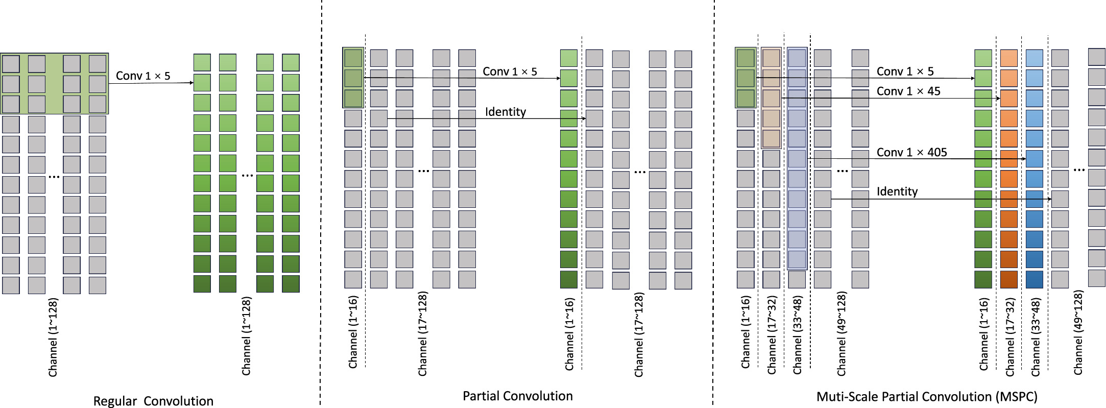
Figure 2. Regular convolution (left panel), partial convolution (middle panel), and multiscale partial convolution (right panel).
Download figure:
Standard image High-resolution imageNevertheless, the utilization of sizable convolution kernels in 1D CNNs necessitates substantial computational resources, resulting in protracted training durations and the potential emergence of overfitting concerns. Subsequently, the forthcoming Section (3.2) will elaborate on strategies employed to mitigate these challenges.
3.2. Multiscale Partial Convolution
In their respective studies, Han et al. (2020) and Zhang et al. (2020) demonstrated that convolutional models often acquire redundant information across various channels, rendering them susceptible to overfitting. The issue of high redundancy in features extracted by regular convolutions for spectra is elaborated in Section 5. Addressing this concern, Chen et al. (2023) introduced Partial Convolution, a technique that selectively applies convolution to a portion of the input channel to extract spatial characteristics while leaving the remainder untouched. This approach offers a viable solution for the model to acquire essential information while significantly reducing computational demands.
In this study, we present the multiscale partial convolution structure, which amalgamates the principles of grouped convolution (Ioannou et al. 2017; Xie et al. 2017; Wang et al. 2023b), partial convolution (Chen et al. 2023), and large-kernel convolution (Ding et al. 2022; Guo et al. 2022; Liu et al. 2022). Figure 2 displays the structures of regular convolution, partial convolution, and multiscale partial convolution (MSPC). Regular Convolution applies convolution operations with small kernels to all channels. Partial Convolution, on the other hand, selectively applies small convolution kernels to specific channels while leaving the remaining channels unaltered. MSPC performs convolution of different-sized convolution kernels for different parts of the channels by group convolution and does not perform any operation on the remaining channels. As depicted in Figure 2 (right panel), MSPC judiciously employs convolution operations on specific channels, facilitating the acquisition of features at various scales through group convolution. This architectural choice empowers the model to encompass both global and local information while mitigating redundancy in feature acquisition.
Furthermore, Equation (3) demonstrates that our approach does not significantly increase the computation complexity compared to the regular 1D CNN, despite using larger convolution kernel size, denoted by k1, k2, and k3 in this study (5, 45, and 405, respectively, in this study, which is chosen by performing ablation experiments). Here, l represents the spectral length, and c represents the number of channels.

3.3. Overall Structure and Details of the Model
The comprehensive architecture of our model, multiscale partial convolution net (MSPC-Net), is elucidated in Figure 3. This design draws inspiration from MetaFormer (Yu et al. 2022) and is organized into four stages (although only two are depicted in the figure). The model initiates with an embedding layer, employing a 1×3 convolution with a stride of 1 to augment the number of channels. Subsequently, a merging layer equipped with a 1×3 convolution and stride 2 is applied before each of the last three stages to downsample the features. Within each stage, we incorporate the Token-mixer and Channel-MLP modules.

Figure 3. The MSPC-Net overall architecture: The macroscopic design of the model is based on MetaFormer (Yu et al. 2022), with four stages in this study, stages 3 and 4 are omitted for brevity. Embedding or Merging precedes each stage for encoding and downsampling. Each stage contains a Token-mixer and Channel-MLP.
Download figure:
Standard image High-resolution imageThe Token mixer integrates the previously discussed MSPC structure. To account for the diverse features captured by MSPC across distinct channels, we introduce a channel attention mechanism in the initial segment of Channel-MLP. To optimize the model size, we adopt the efficient channel attention (ECA; Wang et al. 2020) mechanism, which is recognized for its computational efficiency. This decision is further supported by the ablation experiments presented in Table 7(d). Subsequently, we employ an inverted residual structure comprising two 1×1 convolutional layers and the residual structure. The model's output is processed through the Softmax function to obtain each category's probability without undergoing additional corrective operations. Where K represents the total number of categories, and n denotes the index of the current category.

For an exhaustive understanding of the model's design, please consult Table 2. Different model architectures were designed specifically for each data source (SDSS and LAMOST), and each parameter was chosen after several experiments to select the parameter with the best results. The model designed for SDSS is relatively shallow and contains fewer Identity connections in the convolutional part. On the other hand, the model designed for LAMOST is deeper and incorporates more Identity connections in the convolutional part. As a result, both models have a similar overall size.
Table 2. Model Design Details
| Output Size | Layer Name | SDSS | LAMOST | |
|---|---|---|---|---|
| Stage 1 | 128 × 3582 | Conv. embed | 1 × 3, 128, stride 1 | 1 × 3, 128, stride 1 |
| 128 × 3582 | Token mixer |
![$\left[\begin{array}{c}1\times 5,16,\mathrm{stride}\,1\\ 1\times 45,16,\mathrm{stride}\,1\\ 1\times 405,16,\mathrm{stride}\,1\\ \mathrm{Identity},80\end{array}\right]\times 2$](https://content.cld.iop.org/journals/1538-3881/167/6/260/revision1/ajad38aeieqn5.gif)
|
![$\left[\begin{array}{c}1\times 5,8,\mathrm{stride}\,1\\ 1\times 45,8,\mathrm{stride}\,1\\ 1\times 405,8,\mathrm{stride}\,1\\ \mathrm{Identity},104\end{array}\right]\times 4$](https://content.cld.iop.org/journals/1538-3881/167/6/260/revision1/ajad38aeieqn6.gif)
| |
| Stage 2 | 128 × 1790 | Conv. merge | 1 × 3, 128, stride 2 | 1 × 3, 128, stride 2 |
| 128 × 1790 | Token mixer |
![$\left[\begin{array}{c}1\times 5,16,\mathrm{stride}\,1\\ 1\times 45,16,\mathrm{stride}\,1\\ 1\times 405,16,\mathrm{stride}\,1\\ \mathrm{Identity},80\end{array}\right]\times 2$](https://content.cld.iop.org/journals/1538-3881/167/6/260/revision1/ajad38aeieqn7.gif)
|
![$\left[\begin{array}{c}1\times 5,8,\mathrm{stride}\,1\\ 1\times 45,8,\mathrm{stride}\,1\\ 1\times 405,8,\mathrm{stride}\,1\\ \mathrm{Identity},104\end{array}\right]\times 4$](https://content.cld.iop.org/journals/1538-3881/167/6/260/revision1/ajad38aeieqn8.gif)
| |
| Stage 3 | 128 × 894 | Conv. merge | 1 × 3, 128, stride 2 | 1 × 3, 128, stride 2 |
| 128 × 894 | Token mixer |
![$\left[\begin{array}{c}1\times 5,16,\mathrm{stride}\,1\\ 1\times 45,16,\mathrm{stride}\,1\\ 1\times 405,16,\mathrm{stride}\,1\\ \mathrm{Identity},80\end{array}\right]\times 4$](https://content.cld.iop.org/journals/1538-3881/167/6/260/revision1/ajad38aeieqn9.gif)
|
![$\left[\begin{array}{c}1\times 5,8,\mathrm{stride}\,1\\ 1\times 45,8,\mathrm{stride}\,1\\ 1\times 405,8,\mathrm{stride}\,1\\ \mathrm{Identity},104\end{array}\right]\times 8$](https://content.cld.iop.org/journals/1538-3881/167/6/260/revision1/ajad38aeieqn10.gif)
| |
| Stage4 | 128 × 446 | Conv. merge | 1 × 3, 128, stride 2 | 1 × 3, 128, stride 2 |
| 128 × 446 | Token mixer |
![$\left[\begin{array}{c}1\times 5,16,\mathrm{stride}\,1\\ 1\times 45,16,\mathrm{stride}\,1\\ 1\times 405,16,\mathrm{stride}\,1\\ \mathrm{Identity},80\end{array}\right]\times 2$](https://content.cld.iop.org/journals/1538-3881/167/6/260/revision1/ajad38aeieqn11.gif)
|
![$\left[\begin{array}{c}1\times 5,8,\mathrm{stride}\,1\\ 1\times 45,8,\mathrm{stride}\,1\\ 1\times 405,8,\mathrm{stride}\,1\\ \mathrm{Identity},104\end{array}\right]\times 4$](https://content.cld.iop.org/journals/1538-3881/167/6/260/revision1/ajad38aeieqn12.gif)
| |
| Head | 1 × 1024 | AvgPool and conv. | 1 × 1, 1024, stride 1 | 1 × 1, 1024, stride 1 |
| 1 × 1 | Linear | 1024 × number of categories | 1024 × number of categories | |
| Params | 2.1M | 2.2M | ||
Note. Different model architectures are designed specifically for each data source (SDSS and LAMOST), and each parameter is chosen after several experiments to select the parameter with the best results.
Download table as: ASCIITypeset image
4. Experiments and Results
In this section, we assess the performance of the MSPC-Net model on each of the ten datasets from SDSS and LAMOST. To facilitate comparison, we employ 1D SSCNN (Liu et al. 2019) and Rac-Net (Zou et al. 2020) for astronomical spectral classification, alongside a 1D implementation of ConvNeXt (Liu et al. 2022) originally designed for computer vision tasks. These models for comparison can be obtained from the website https://github.com/qintianjian-lab/Spectrum-Classification-Models. Furthermore, we conduct comprehensive ablation experiments to corroborate the efficacy of the MSPC-Net model and validate our design choices.
4.1. Setup
We conduct experiments to evaluate the model's performance using the ten datasets as described in Table 1. The first eight datasets correspond to the ideal case stellar classification and stellar subclass classification, respectively. Additionally, Dataset FC-S and Dataset FC-L are employed to assess the model's performance in practical application scenarios. To ensure the reliability of our experiments, we conduct different fold cross validation on each dataset, with the training set, validation set, and test set divided in a ratio of 6:2:2.
Model Variants: An integral aspect of MSPC-Net's design is its focus on enhancing generalization performance, ensuring consistent and robust results across various spectral datasets. This adaptability hinges on two dynamic parameters: n_div, adjusting the model's width by modifying the partial convolution ratio, and depth_scale, refining the model's depth. Through meticulous fine-tuning of these parameters, we can customize the model's size to suit different datasets, thus optimizing its performance. Consequently, to account for the difference in the data from SDSS and LAMOST, we design distinct model variants for each data source. Table 2 illustrates that in the SDSS model, the Identity component constitutes three-eighths of the MSPC. Conversely, in the LAMOST model, the Identity component comprises three-sixteenths of the total. Despite this difference, both models have a comparable number of parameters, primarily due to the deeper architecture of the LAMOST model. For other surveys, we provide a Python-based data preprocessing utility that simply necessitates modifications to the file reading function. After the data are prepared and processed, users can refine the model's architecture and training parameters through the configuration file, thereby enhancing the model's performance.
Training: for all experiments, we use the Adam optimizer (Kingma & Ba et al. 2015) empirically. The learning rate is adjusted using cosine annealing with warm restarts (Loshchilov & Hutter 2017), starting at 1e-4 and gradually decreasing to 1e-8, which is chosen after several experiments. In addition, we empirically add a random depth (Huang et al. 2016). Cross-entropy loss function is utilized.
Environment: all codes are implemented in Python 3.9 using PyTorch 2.0 and executed on hardware with an i9-13900K processor and RTX-4080 graphics card.
4.2. Results
We evaluate each model's performance using accuracy and F1-score as metrics. The cross-validation results for all models on the eight datasets with different folds are presented in Tables 3–4. First, let us delve into stellar classification. As shown in Table 3, MSPC-Net outperforms the other models. Transitioning to stellar subclass classification, it is noteworthy that, as depicted in Table 4, MSPC-Net excels in terms of both accuracy and F1-score across all four datasets, despite having similar parameters. We provide category-specific details in Table 5 to facilitate a comprehensive comparison of the model's performance. These details include true positive, false negative top-1, and false positive top-1 values for Dataset SS-S (>5). Due to space limitations, we exclusively compare SSCNN and MSPC-Net, where MSPC-Net outperforms SSCNN across most categories.
Table 3. Accuracy and F1-score on Stellar Classification
| Model | Size | Accuracy (%) | F1-score (%) | ||||||||||
|---|---|---|---|---|---|---|---|---|---|---|---|---|---|
| fold1 | fold2 | fold3 | fold4 | fold5 | Avg | fold1 | fold2 | fold3 | fold4 | fold5 | Avg | ||
| Dataset SC-S (>5) | |||||||||||||
| SSCNN | 7.5 M | 84.89 | 85.29 | 85.64 | 84.39 | 86.54 | 85.35 | 84.78 | 85.21 | 85.55 | 84.34 | 86.51 | 85.28 |
| RACNet | 759.2 K | 85.29 | 85.93 | 85.71 | 84.39 | 85.89 | 85.44 | 85.23 | 85.89 | 85.59 | 84.41 | 85.90 | 85.40 |
| ConvNeXt | 573.2 K | 85.14 | 84.39 | 83.25 | 82.04 | 84.14 | 83.79 | 85.04 | 84.33 | 82.85 | 81.87 | 84.11 | 83.64 |
| MSPC-Net | 2.1 M | 87.82 | 86.68 | 88.04 | 86.71 | 87.96 | 87.74 | 87.76 | 86.69 | 87.95 | 86.62 | 87.96 | 87.39 |
| Dataset SC-S (>10) | |||||||||||||
| SSCNN | 7.5 M | 88.07 | 89.00 | 89.39 | 88.89 | 88.89 | 88.65 | 87.90 | 88.91 | 88.32 | 88.84 | 88.88 | 88.57 |
| RACNet | 759.2 K | 88.82 | 87.68 | 87.39 | 86.96 | 87.96 | 87.76 | 88.78 | 87.64 | 87.39 | 86.90 | 87.90 | 87.72 |
| ConvNeXt | 573.2 K | 85.46 | 87.36 | 86.96 | 87.07 | 86.32 | 86.64 | 85.30 | 87.26 | 86.91 | 86.99 | 86.25 | 86.54 |
| MSPC-Net | 2.1 M | 89.86 | 89.79 | 90.46 | 89.04 | 91.18 | 90.06 | 89.78 | 89.74 | 90.42 | 88.99 | 91.12 | 90.01 |
| Dataset SC-L (>5) | |||||||||||||
| SSCNN | 7.5 M | 88.92 | 89.08 | 89.67 | 88.38 | 89.08 | 89.02 | 88.94 | 89.09 | 89.64 | 88.35 | 89.05 | 89.01 |
| RACNet | 759.2 K | 87.71 | 88.71 | 87.21 | 87.63 | 87.88 | 87.83 | 87.75 | 88.71 | 87.15 | 87.61 | 87.86 | 87.82 |
| ConvNeXt | 573.2 K | 88.79 | 89.17 | 89.54 | 87.63 | 88.63 | 88.75 | 88.82 | 89.17 | 89.53 | 87.71 | 88.65 | 88.77 |
| MSPC-Net | 2.2 M | 90.08 | 89.79 | 89.17 | 89.25 | 88.96 | 89.45 | 90.09 | 89.81 | 89.14 | 89.24 | 88.94 | 89.44 |
| Dataset SC-L (>10) | |||||||||||||
| SSCNN | 7.5 M | 90.63 | 90.96 | 89.79 | 90.96 | 90.79 | 90.63 | 90.57 | 90.96 | 89.75 | 90.94 | 90.81 | 90.61 |
| RACNet | 759.2 K | 89.00 | 90.63 | 89.42 | 89.08 | 89.96 | 89.62 | 89.02 | 90.62 | 89.42 | 89.08 | 89.97 | 89.62 |
| ConvNeXt | 573.2 K | 89.46 | 90.50 | 89.67 | 90.50 | 90.25 | 90.07 | 89.43 | 90.46 | 89.68 | 90.53 | 90.27 | 90.07 |
| MSPC-Net | 2.2 M | 90.00 | 91.83 | 90.04 | 90.33 | 91.71 | 90.78 | 89.95 | 91.80 | 90.04 | 90.34 | 91.70 | 90.77 |
Note. The sections that exhibit strong performance have been highlighted in bold.
Download table as: ASCIITypeset image
Table 4. Accuracy and F1-score on Stellar Subclass Classification
| Model | Size | Accuracy (%) | F1-score (%) | ||||||||||
|---|---|---|---|---|---|---|---|---|---|---|---|---|---|
| fold1 | fold2 | fold3 | fold4 | fold5 | Avg | fold1 | fold2 | fold3 | fold4 | fold5 | Avg | ||
| Dataset SS-S (>5) | |||||||||||||
| SSCNN | 7.5 M | 79.87 | 79.06 | 78.84 | 79.09 | 79.19 | 79.21 | 79.85 | 78.96 | 78.70 | 79.02 | 79.18 | 79.14 |
| RACNet | 759.2 K | 79.95 | 79.39 | 78.78 | 79.74 | 78.99 | 79.37 | 79.98 | 79.38 | 78.58 | 79.70 | 78.98 | 79.32 |
| ConvNeXt | 573.2 K | 77.35 | 76.93 | 77.06 | 77.28 | 76.98 | 77.12 | 77.31 | 76.87 | 77.02 | 77.25 | 76.97 | 77.09 |
| MSPC-Net | 2.1 M | 82.18 | 82.32 | 83.17 | 82.86 | 82.38 | 82.58 | 82.03 | 82.20 | 83.04 | 82.70 | 82.27 | 82.45 |
| Dataset SS-S (>10) | |||||||||||||
| SSCNN | 7.5 M | 82.14 | 82.64 | 82.78 | 83.24 | 82.99 | 82.76 | 82.13 | 82.65 | 82.72 | 83.13 | 82.97 | 82.72 |
| RACNet | 759.2 K | 82.67 | 82.24 | 81.91 | 83.01 | 81.32 | 82.23 | 82.69 | 82.24 | 81.87 | 82.98 | 81.41 | 82.24 |
| ConvNeXt | 573.2 K | 81.80 | 81.59 | 81.59 | 82.70 | 81.35 | 81.81 | 81.79 | 81.60 | 81.51 | 82.62 | 81.38 | 81.78 |
| MSPC-Net | 2.1 M | 86.37 | 86.02 | 85.12 | 85.52 | 85.93 | 85.79 | 86.29 | 85.97 | 85.11 | 85.44 | 85.91 | 85.74 |
| Dataset SS-L (>5) | |||||||||||||
| SSCNN | 7.5 M | 65.42 | 66.34 | 65.23 | 65.54 | 65.72 | 65.65 | 65.43 | 65.34 | 65.22 | 65.51 | 65.72 | 65.65 |
| RACNet | 759.2 K | 67.13 | 68.80 | 67.85 | 66.88 | 68.97 | 67.93 | 67.11 | 68.78 | 67.89 | 66.88 | 68.98 | 67.93 |
| ConvNeXt | 573.2 K | 67.76 | 68.41 | 67.70 | 68.14 | 68.07 | 68.01 | 67.77 | 68.39 | 67.66 | 68.12 | 68.06 | 68.00 |
| MSPC-Net | 2.2 M | 71.87 | 72.01 | 71.61 | 71.20 | 71.64 | 71.67 | 71.88 | 72.01 | 71.64 | 71.25 | 71.67 | 71.69 |
| Dataset SS-L (>10) | |||||||||||||
| SSCNN | 7.5 M | 68.93 | 69.43 | 69.39 | 70.04 | 68.73 | 69.30 | 68.93 | 69.40 | 69.38 | 70.00 | 68.67 | 69.28 |
| RACNet | 759.2 K | 68.89 | 70.74 | 71.38 | 70.87 | 71.64 | 70.70 | 68.85 | 70.73 | 71.36 | 70.84 | 71.58 | 70.67 |
| ConvNeXt | 573.2 K | 71.18 | 71.55 | 72.02 | 72.06 | 71.76 | 71.71 | 71.15 | 71.55 | 71.99 | 72.03 | 71.71 | 71.68 |
| MSPC-Net | 2.2 M | 75.01 | 75.09 | 75.06 | 75.09 | 74.40 | 74.93 | 74.99 | 75.08 | 75.05 | 75.06 | 74.38 | 74.91 |
Note. The sections that exhibit strong performance have been highlighted in bold.
Download table as: ASCIITypeset image
Table 5. Details of the Classification Results of Each Category of SSCNN and MSPC-Net on Dataset SS-S (>5)
| SSCNN | MSPC-Net | ||||
|---|---|---|---|---|---|
| TP | FN (top-1) | FP (top-1) | TP | FN (top-1) | FP (top-1) |
| A0 (372) | F5→A0 (22) | A0→F5 (22) | A0 (375) | F5→A0 (24) | A0→F5 (19) |
| A2 (290) | F0→A2 (75) | A2→F0 (60) | A2 (320) | F0→A2 (54) | A2→F0 (79) |
| A4 (362) | F0→A4 (16) | A4→F0 (17) | A4 (357) | A2→A4 (27) | A4→F0 (12) |
| F0 (288) | A2→F0 (60) | F0→A2 (75) | F0 (283) | A2→F0 (79) | F0→A2 (54) |
| F2 (229) | G0→F2 (70) | F2→G0 (70) | F2 (268) | G0→F2 (41) | F2→G0 (78) |
| F3 (331) | F0→F3 (28) | F3→F0 (25) | F3 (333) | F0→F3 (33) | F3→F0 (18) |
| F5 (326) | F2→F5 (41) | F5→F2 (36) | F5 (344) | F2→F5 (34) | F5→F2 (29) |
| F8 (303) | G0→F8 (41) | F8→G0 (47) | F8 (331) | G4→F8 (33) | F8→G0 (52) |
| F9 (336) | G2→F9 (41) | F9→G2 (26) | F9 (346) | G2→F9 (35) | F9→K1 (17) |
| G0 (162) | F2→G0 (70) | G0→F2 (70) | G0 (153) | F2→G0 (78) | G0→G2 (58) |
| G2 (299) | G0→G2 (53) | G2→G0 (58) | G2 (310) | G0→G2 (58) | G2→G0 (46) |
| G4 (288) | F8→G4 (41) | G4→G8 (41) | G4 (325) | F8→G4 (33) | G4→G8 (45) |
| G5 (343) | K1→G5 (19) | G5→K1 (27) | G5 (347) | K1→G5 (19) | G5→K1 (31) |
| G8 (250) | K0→G8 (94) | G8→K0 (82) | G8 (275) | K0→G8 (72) | G8→K0 (80) |
| K0 (264) | G8→K0 (82) | K0→G8 (94) | K0 (287) | G8→K0 (80) | K0→G8 (72) |
| K1 (328) | G5→K1 (27) | K1→K3 (28) | K1 (332) | G5→K1 (31) | K1→K3 (24) |
| K3 (311) | K1→K3 (28) | K3→K5 (21) | K3 (312) | G5→K3 (24) | K3→K5 (17) |
| K5 (335) | K7→K5 (32) | K5→K3 (27) | K5 (340) | K7→K5 (29) | K5→K3 (24) |
| K7 (358) | K5→K7 (21) | K7→K5 (32) | K7 (380) | M0→K7 (15) | K7→K5 (29) |
| M0 (363) | M1→M0 (21) | M0→K7 (20) | M0 (380) | M1→M0 (13) | M0→M1 (18) |
| M1 (340) | M2→M1 (26) | M1→M2 (24) | M1 (355) | M2→M1 (18) | M1→M0 (13) |
| M2 (343) | M3→M2 (26) | M2→M3 (29) | M2 (372) | M3→M2 (21) | M2→M1 (18) |
| M3 (345) | M2→M3 (29) | M3→M4 (30) | M3 (376) | M4→M3 (15) | M3→M4 (22) |
| M4 (332) | M5→M4 (34) | M4→M5 (25) | M4 (359) | M3→M4 (22) | M4→M5 (38) |
| M5 (369) | M4→M5 (25) | M5→M4 (34) | M5 (358) | M4→M5 (38) | M5→M4 (16) |
Note. The total number for each category is 400. In terms of performance, the ideal scenario is when true positive (TP) values are higher and better, while false negative (FN) and false oositive (FP) values are lower and better. The sections that exhibit strong performance have been highlighted in bold.
Download table as: ASCIITypeset image
To further validate the model's feature extraction capability, we conduct data dimensionality reduction using t-SNE (Wattenberg et al. 2016; Ma et al. 2022) for all model-extracted features and visually represent the results. In Figure 4 (left panel), we showcase the feature visualization of Dataset SS-S (>10), focusing solely on five out of the 24 categories, for illustrative purpose. It is discernible that all models encounter difficulty in distinguishing between G0 and K0, which aligns with the low true positive quantity for G0 in Table 5. This result is consistent with findings reported by Liu et al. (2015), suggesting a minimal distinction between late G-type stars and early K-type stars. However, in the remaining three categories, notably F0, MSPC-Net outperforms all other models, underscoring MSPC-Net's advantage in feature extraction. For Dataset SS-L (>10), we visualize four out of the categories in Figure 4, and the overall differentiation is not as pronounced as in Dataset SS-S (>10). MSPC-Net notably exhibits a more robust feature extraction ability than other models for Dataset SS-L (>10).

Figure 4. The t-SNE visualizations of the samples (5 class for Dataset SS-S (>10) and 4 class for Dataset SS-L (>10)) generated by different models. Features extracted for the Dataset SS-S (>10) (left panel) and Dataset SS-L (>10) (right panel) models are downscaled and visualized by t-SNE. The red rectangle highlights the area of the clustering error. For Dataset SS-S (>10), all models perform poorly in distinguishing between G0 and K0, but the MSPC-Net outperforms the other models for the other data types. For Dataset SS-L (>10), all models do not discriminate clearly between A0 and other data, and overall, MSPC-Net clustering is better than the other models.
Download figure:
Standard image High-resolution imageFollowing the evaluation of MSPC-Net under ideal conditions (sample average; high S/N), we test each modelon Dataset FC-S and Dataset FC-L, which closely emulate practical application scenarios. As demonstrated in Table 6, the results consistently reveal MSPC-Net's superiority across all metrics, affirming its exceptional applicability in practical application scenarios. It is important to note that the relatively low F1-score for each model on Dataset FC-S is attributable to the sample's extreme imbalance.
Table 6. Accuracy and F1-score on Full Classification
| Model | Size | Accuracy (%) | F1-score (%) | ||||||||||
|---|---|---|---|---|---|---|---|---|---|---|---|---|---|
| fold1 | fold2 | fold3 | fold4 | fold5 | Avg | fold1 | fold2 | fold3 | fold4 | fold5 | Avg | ||
| Dataset FC-S | |||||||||||||
| SSCNN | 7.5 M | 55.05 | 55.02 | 54.75 | 55.83 | 55.27 | 55.18 | 50.89 | 51.04 | 50.37 | 51.67 | 50.89 | 50.97 |
| RACNet | 759.2 K | 57.22 | 57.89 | 57.99 | 58.18 | 57.47 | 57.75 | 53.00 | 53.40 | 53.37 | 53.70 | 53.22 | 53.34 |
| ConvNeXt | 573.2 K | 53.30 | 53.77 | 53.89 | 53.94 | 54.45 | 53.87 | 49.04 | 49.17 | 49.53 | 49.56 | 50.03 | 49.47 |
| MSPC-Net | 2.1 M | 60.75 | 60.83 | 60.91 | 60.90 | 61.24 | 60.93 | 56.23 | 56.09 | 56.12 | 56.26 | 56.57 | 56.25 |
| Dataset FC-L | |||||||||||||
| SSCNN | 7.5 M | 66.55 | 65.61 | 65.91 | 66.20 | 67.04 | 66.26 | 66.56 | 65.65 | 66.04 | 66.18 | 67.04 | 66.29 |
| RACNet | 759.2 K | 68.11 | 67.41 | 67.72 | 67.92 | 67.98 | 67.83 | 68.07 | 67.47 | 67.76 | 67.96 | 68.03 | 67.86 |
| ConvNeXt | 573.2 K | 68.49 | 68.10 | 67.99 | 68.77 | 68.54 | 68.38 | 68.43 | 68.12 | 68.08 | 68.74 | 68.53 | 68.38 |
| MSPC-Net | 2.2 M | 72.75 | 71.67 | 72.09 | 72.34 | 72.35 | 72.24 | 72.71 | 71.73 | 72.20 | 72.30 | 72.39 | 72.27 |
Note. The sections that exhibit strong performance have been highlighted in bold.
Download table as: ASCIITypeset image
To further substantiate the impact of S/N on model accuracy, as depicted in Figure 5, we present the distribution of S/N for Dataset FC-S and Dataset FC-L, alongside the corresponding accuracy of each model. It is discernible that the majority of data in Dataset FC-S has a relatively low S/N, whereas the S/N for the data in Dataset FC-L exhibits a marked improvement. We speculate that this dissimilarity in S/N distribution accounts for the notable disparity in accuracy between these two datasets. Moreover, MSPC-Net consistently outperforms alternative models across most S/N intervals in both datasets, underscoring its exceptional performance and robustness.

Figure 5. Accuracy as a function of S/N interval (upper panels) and the S/N distribution (lower panels), left panels for Dataset FC-S and right panels for Dataset FC-L.
Download figure:
Standard image High-resolution image4.3. Ablation Study
Several ablation experiments are conducted to assess the effectiveness of each component in our model. We conducted ablation experiments across all datasets, with a particular emphasis on showcasing the results for Dataset SS-S (> 5). Detailed results of the ablation experiments for the remaining datasets can be found in Appendix A.
Partial convolution: as depicted in Table 7(a), the Identity ratio (the proportion of channels without any operation in the convolution) is presented. As the ratio increases, the model size gradually decreases, while the accuracy and F1-score of the model increase, affirming the effectiveness of partial convolution. For the dataset sourced from SDSS, a ratio of 5/8 is utilized, while a ratio of 13/16 is employed for the dataset sourced from LAMOST.
Table 7. Ablation Study
| Identity Ratio | Model Size | Acc (%) | F1 (%) |
|---|---|---|---|
| 0 | 9.0 M | 82.07 | 82.00 |
| 1 / 4 | 5.6 M | 81.52 | 81.42 |
| 5 / 8 | 2.1 M | 82.18 | 82.03 |
| 13 / 16 | 1.3 M | 82.00 | 81.87 |
| (a) Partial convolution | |||
| Convolution Kernel Size | Model Size | Acc (%) | F1 (%) |
|---|---|---|---|
| 1 × 3, 1 × 3, 1 × 3 | 989.1 K | 72.24 | 71.87 |
| 1 × 3, 1 × 9, 1 × 27 | 1.1 M | 78.29 | 78.10 |
| 1 × 3, 1 × 27, 1 × 243 | 1.7 M | 81.83 | 81.74 |
| 1 × 5, 1 × 5, 1 × 5 | 1.0 M | 72.52 | 72.25 |
| 1 × 5, 1 × 15, 1 × 45 | 1.1 M | 78.91 | 78.72 |
| 1 × 5, 1 × 45, 1 × 405 | 2.1 M | 82.18 | 82.03 |
| (b) Multiscale large-kernel convolution. | |||
| Channels | Model Size | Acc (%) | F1 (%) |
|---|---|---|---|
| 64 | 586.4 K | 80.78 | 80.61 |
| 128 | 2.1 M | 82.18 | 82.03 |
| 256 | 8.2 M | 82.60 | 82.55 |
| (c) Channels. | |||
| Attention | Model Size | Acc (%) | F1 (%) |
|---|---|---|---|
| None | 2.1 M | 81.70 | 81.58 |
| ECA | 2.1 M | 82.18 | 82.03 |
| (d) Attention. | |||
Note. Ablation experiments on Dataset SS-S (>5). (a) Partial convolution. The ratio of identity, 5/8, works best. (b) Multiscale large-kernel convolution. 1 × 5, 1 × 45, and 1 × 405 kernel combinations of different sizes give the best results. (c) Channels. 256 gives the best results, but 128 is chosen for performance and efficiency. (d) Attention. Better results with ECA attention. The best performance is in bold and the model setting is adopted with a gray background in this study.
Download table as: ASCIITypeset image
Token-mixer and Channel-MLP: in Table 7(b), we showcase the performance of various multiscale convolutional kernels. In comparison to conventional 1×3 and 1×5 convolutions, our multiscale convolutional kernel demonstrates a notable enhancement in performance without a substantial increase in the parameter number. Furthermore, we validate the importance of the ECA attention mechanism, as elucidated in Table 7(d). The model's size remains nearly unchanged with the incorporation of ECA, while the performance is also partially improved.
Channels: given the critical role of the number of channels in CNN-based models, we conduct comparative experiments for different channel numbers, as outlined in Table 7(c). Although a channel number of 256 yields better performance, considering both performance and efficiency, the default channel number used in this study is 128.
5. Discussion
In Section 1, we propose that recent approaches of spectral classification might be prone to overfitting due to redundant features in their models. To validate this hypothesis, we visually illustrate the accuracy of the training set and the validation set of all models during their training process on Dataset SS-S (>5) in Figure 6. As shown in Figure 6, accuracy improves with the increase of epoch for the whole trend, and only there are two sudden decreases for the training dataset which is due to the warm-up learning rate adjustment strategy. Except for MSPC-Net, each model exhibits very significant overfitting. The epoch less than 100 is due to the use of early stopping. We observe varying degrees of overfitting in SSCNN models with larger sizes compared to MSPC-Net, RACNet, and ConvNeXt models with smaller sizes than MSPC-Net. Notably, MSPC-Net demonstrates a higher degree of resilience to overfitting than the other models.

Figure 6. Training accuracy (left panel) and validation accuracy (right panel) curves with different epochs for each model.
Download figure:
Standard image High-resolution imageTo deepen our comprehension of MSPC-Net's remarkable performance, we provide a visualization of the model's learning representation in Figure 7. By leveraging a multiscale convolutional kernel and partial convolution, MSPC-Net can acquire distinctive features in different channels. In contrast, the regular convolutional model extracts similar features across channels, implying the existence of redundant features that contribute to its subpar performance and susceptibility to overfitting.

Figure 7. Feature visualization. Regular convolution and MSCP-Net extract the features of the spectrum, with the horizontal axis indicating the length of the features and the vertical axis indicating the features of the different channels. Unlike the regular convolution, where the features of each channel are very similar, the features of each channel of MSPC-Net show diversity. This visualization highlights the feature extraction capabilities of the multiscale large-kernel convolution (channels 1 to 48) and partial convolution (channels 49 to 128) within the MSPC module. The former illustrates the diversity of extracted features, while the latter showcases reduced parameter count, notably with the Identity function requiring no additional parameters.
Download figure:
Standard image High-resolution imageAdditionally, we conduct an in-depth analysis of the test set from Dataset SC-S (>5). We cross-match the 2,800 stars in the test set with the LAMOST DR10 catalog within a two-arcsecond radius and identify 329 corresponding labels from the LAMOST pipeline. We then categorize these data into two groups: 301 agree with MSPC-Net's predictions, matching the SDSS labels (considered correct predictions), while 28 show discrepancies (considered incorrect predictions). As illustrated in Figure 8, comparing the SDSS and LAMOST labels for these two subsets of data reveals that the consistency in the MSPC-Net correct prediction group is significantly higher than in the incorrect prediction group.

Figure 8. Label consistency of SDSS and LAMOST in the group correct predictions (left panel) and the group incorrect predictions (right panel).
Download figure:
Standard image High-resolution imageUpon closer examination of the cases where predictions are inaccurate, most of MSPC-Net's misclassifications (20 out of 28) occur in instances where the classification systems of SDSS and LAMOST are inconsistent. Furthermore, these misclassifications often align with the labels provided by LAMOST (17 out of 28). This observation suggests that MSPC-Net has the potential to identify spectra prone to misclassification, facilitating subsequent corrections.
Additionally, we conduct a visual inspection of these 28 spectra, Figure 9 shows an example of one of these, the full 28 spectra are available in the online journal. The outcomes of this inspection are categorized as follows:
- 1.MSPC-Net's correct predictions where SDSS labels are incorrect (15 instances).
- 2.Cases are hard to judge due to sources lying in the transition between two neighboring subclasses (two instances).
- 3.Instances where MSPC-Net's predictions are incorrect while SDSS labels are accurate (seven instances).
- 4.Low-quality spectra (four instances), with two of them confirmed by LAMOST spectra to have been accurately predicted by MSPC-Net.

Figure 9.
An example of MSPC-Net's incorrect predictions. A-type labeled by SDSS, F-type labeled by LAMOST, F-type predicted by MSPC-Net, and then identified as F-type after visual inspection. The templates and spectrum of SDSS are officially provided by SDSS, while the spectrum of LAMOST is officially provided by LAMOST. The complete figure set (28 images) is available in the online journal. (The complete figure set (28 images) is available.)
Download figure:
Standard image High-resolution imageMSPC-Net demonstrates remarkable performance when applied to SDSS and LAMOST datasets, effectively tackling various spectral classification tasks using extensive labeled data. As depicted in Figure 5, its superiority becomes evident particularly in handling low-S/N data, surpassing competing models. This capability fills a crucial gap where traditional template matching methods falter. However, despite these merits, MSPC-Net's reliance on vast labeled datasets presents challenges in specific astronomical tasks. Unlike the more universally adaptable template matching approach, MSPC-Net necessitates retraining due to the typically diverse data sourced from various sky surveys, thereby limiting its versatility across different surveys. Moreover, akin to other deep-learning methodologies, MSPC-Net encounters issues related to limited interpretability. In our forthcoming endeavors, we aim to enhance MSPC-Net's capabilities through transfer learning techniques(Kolesnikov et al. 2020; Tan et al. 2023) to diminish its dependence on extensive labeled datasets and augment its adaptability across diverse surveys. Additionally, we are actively developing an interactive exploration tool to enhance the interpretability of deep-learning models, thereby broadening their applicability in the domain of astronomical spectroscopy.
6. Conclusion
This study introduces MSPC-Net, a novel spectral classification method that addresses the limitations of existing astronomical spectral classification models, especially in general datasets. Extensive experiments demonstrate that MSPC-Net brings significant improvements to model classification performance. The proposed method leverages large-kernel and MSPC techniques to enhance accuracy. To reduce the model's parameter number and mitigate overfitting, partial convolution is employed, selectively excluding specific channels from the convolution operation. Experimental results validate that this approach not only improves model performance but also reduces the number of parameters. Furthermore, the combination of large-kernel convolution and group convolution creates an MSPC block capable of extracting both local and global features, leading to substantial enhancements in model performance. Additionally, the use of grouped convolution ensures that each channel represents distinct features, and the introduction of the ECA mechanism enables the model to learn feature importance without affecting the parameter number. Experimental validation confirms the effectiveness of these strategies.
To validate the model's performance, we create ten datasets from SDSS DR18 and LAMOST DR10. These datasets represent different aspects of celestial object classification, including stellar subclass classification, stellar classification, and full classification. To create the stellar classification and stellar subclass classification datasets, we filter the data based on the S/N threshold and the number of samples per category. On the other hand, the full classification dataset is randomly chosen without any specific restrictions. We are able to test the model's performance in both ideal and practical application scenarios with these datasets. All of these datasets are further divided into training, test, and validation sets, and we have made them open-source for future use. By doing so, we hope that other researchers and practitioners can also evaluate the performance of their models using these datasets expediently. The results of our evaluation show that all MSPC-Net models performed well in the stellar classification dataset, which has a smaller number of categories. However, in the stellar subclass classification dataset, which has a larger number of categories, as well as in the full classification dataset, our models demonstrate significant performance advantages. These results confirm the effectiveness and robustness of our MSPC-Net model in all applications. Due to its robust feature extraction capabilities and adaptable nature, MSPC-Net holds potential for a wide array of spectral data analysis tasks (e.g., spectral classification and identification of rare celestial objects).
Our work shed light on the generalization problem of classification models when faced with a diverse range of astronomical spectra. By demonstrating the effectiveness of MSPC-Net across various datasets, we contribute valuable insights to the development of robust and versatile classification models for large sky surveys. In summary, our work on MSPC-Net represents a significant advancement in the automated classification of astronomical spectra, offering a solution that excels in performance across diverse datasets. The thorough experimentation and analysis further strengthen the credibility of our findings and highlight the potential applications of our method in large-scale spectroscopic sky survey projects (e.g., LAMOST, SDSS, and DESI).
Acknowledgments
We greatly appreciate the valuable comments and suggestions from the reviewer. The study is funded by the National Natural Science Foundation of China under grants Nos. 12273076 and 12133001, the China Manned Space Project, with science research grant Nos. CMS-CSST-2021-A04 and CMS-CSST-2021-A06 and Shenzhen Fundamental Research Program (JCYJ20230807094104009). GuoShouJing Telescope (LAMOST) is a National Major Scientific Project built by the Chinese Academy of Sciences. Funding for the Sloan Digital Sky Survey IV has been provided by the Alfred P. Sloan Foundation, the U.S. Department of Energy Office of Science, and the Participating Institutions. SDSS-IV acknowledges support and resources from the Center for High-Performance Computing at the University of Utah. The SDSS website is www.sdss.org. SDSS-IV is managed by the Astrophysical Research Consortium for the Participating Institutions of the SDSS Collaboration including the Brazilian Participation Group, the Carnegie Institution for Science, Carnegie Mellon University, the Chilean Participation Group, the French Participation Group, Harvard-Smithsonian Center for Astrophysics, Instituto de Astrofísica de Canarias, The Johns Hopkins University, Kavli Institute for the Physics and Mathematics of the Universe (IPMU) /University of Tokyo, Lawrence Berkeley National Laboratory, Leibniz Institut für Astrophysik Potsdam (AIP), Max-Planck-Institut für Astronomie (MPIA Heidelberg), Max-Planck-Institut für Astrophysik (MPA Garching), Max-Planck-Institut für Extraterrestrische Physik (MPE), National Astronomical Observatories of China, New Mexico State University, New York University, University of Notre Dame, Observatário Nacional / MCTI, The Ohio State University, Pennsylvania State University, Shanghai Astronomical Observatory, United Kingdom Participation Group, Universidad Nacional Autónoma de México, University of Arizona, University of Colorado Boulder, University of Oxford, University of Portsmouth, University of Utah, University of Virginia, University of Washington, University of Wisconsin, Vanderbilt University, and Yale University. We acknowledge the use of spectra from LAMOST and SDSS.
Data Availability
The code and data associated with this research are publicly available at (https://github.com/qintianjian-lab/MSPC-Net), LAMOST (https://www.lamost.org), SDSS (https://www.sdss.org), and China-VO (doi:10.12149/101370).
Appendix A: Complete Ablation Experiments
We conduct ablation experiments on all datasets, and the experimental results are shown in the following tables: Dataset SC-S (Tables 8 and 9), Dataset SS-S (Tables 10 and 11), Dataset FC-S (Table 12), Dataset SC-L (Tables 13 and 14), Dataset SS-L (Tables 15 and 16), Dataset FC-L (Table 17). The above tables all highlight the best performance in bold.
Table 8. Ablation Experiment on Dataset SC-S (>5)
| Model Parameter | Metrics | |||||
|---|---|---|---|---|---|---|
| Identity Ratio | Convolution Kernel Size | Channels | Attention | Model Size | Accuracy (%) | F1-score (%) |
| 0 | 1 × 5, 1 × 45, 1 × 405 | 128 | ECA | 9.0 M | 86.54 | 86.46 |
| 1 / 4 | 1 × 5, 1 × 45, 1 × 405 | 128 | ECA | 5.6 M | 87.18 | 87.14 |
| 5 / 8 | 1 × 5, 1 × 45, 1 × 405 | 128 | ECA | 2.1 M | 87.71 | 87.64 |
| 13 /16 | 1 × 5, 1 × 45, 1 × 405 | 128 | ECA | 1.3 M | 86.04 | 85.93 |
| 5 / 8 | 1 × 3, 1 × 3, 1 × 3 | 128 | ECA | 989.1 K | 81.82 | 81.58 |
| 5 / 8 | 1 × 3, 1 × 9, 1 × 27 | 128 | ECA | 1.1 M | 86.14 | 86.08 |
| 5 / 8 | 1 × 3, 1 × 27, 1 × 243 | 128 | ECA | 1.7 M | 86.89 | 86.81 |
| 5 / 8 | 1 × 5, 1 × 5, 1 × 5 | 128 | ECA | 1.0 M | 80.54 | 80.21 |
| 5 / 8 | 1 × 5, 1 × 15, 1 × 4 | 128 | ECA | 1.1 M | 86.50 | 86.41 |
| 5 / 8 | 1 × 5, 1 × 45, 1 × 405 | 128 | ECA | 2.1 M | 87.71 | 87.64 |
| 5 / 8 | 1 × 5, 1 × 45, 1 × 405 | 64 | ECA | 586.4 K | 85.00 | 84.90 |
| 5 / 8 | 1 × 5, 1 × 45, 1 × 405 | 128 | ECA | 2.1 M | 87.71 | 87.64 |
| 5 / 8 | 1 × 5, 1 × 45, 1 × 405 | 256 | ECA | 8.2 M | 88.07 | 88.00 |
| 5 / 8 | 1 × 5, 1 × 45, 1 × 405 | 128 | None | 2.1 M | 87.07 | 87.01 |
| 5 / 8 | 1 × 5, 1 × 45, 1 × 405 | 128 | ECA | 2.1 M | 87.71 | 87.64 |
Download table as: ASCIITypeset image
Table 9. Ablation Experiment on Dataset SC-S (>10)
| Model Parameter | Metrics | |||||
|---|---|---|---|---|---|---|
| Identity Ratio | Convolution Kernel Size | Channels | Attention | Model Size | Accuracy (%) | F1-score (%) |
| 0 | 1 × 5, 1 × 45, 1 × 405 | 128 | ECA | 9.0 M | 86.50 | 86.40 |
| 1 / 4 | 1 × 5, 1 × 45, 1 × 405 | 128 | ECA | 5.6 M | 88.07 | 88.00 |
| 5 / 8 | 1 × 5, 1 × 45, 1 × 405 | 128 | ECA | 2.1 M | 89.89 | 89.81 |
| 13 /16 | 1 × 5, 1 × 45, 1 × 405 | 128 | ECA | 1.3 M | 88.64 | 88.56 |
| 5 / 8 | 1 × 3, 1 × 3, 1 ×3 | 128 | ECA | 989.1 K | 83.00 | 82.71 |
| 5 / 8 | 1 × 3, 1 × 9, 1 × 27 | 128 | ECA | 1.1 M | 87.61 | 87.55 |
| 5 / 8 | 1 × 3, 1 × 27, 1 × 243 | 128 | ECA | 1.7 M | 88.82 | 88.76 |
| 5 / 8 | 1 × 5, 1 × 5, 1 × 5 | 128 | ECA | 1.0 M | 83.00 | 82.76 |
| 5 / 8 | 1 × 5, 1 × 15, 1 × 4 | 128 | ECA | 1.1 M | 86.64 | 86.54 |
| 5 / 8 | 1 × 5, 1 × 45, 1 × 405 | 128 | ECA | 2.1 M | 89.89 | 89.81 |
| Ccolspan1-7 | ||||||
| 5 / 8 | 1 × 5, 1 × 45, 1 × 405 | 64 | ECA | 586.4 K | 86.57 | 86.48 |
| 5 / 8 | 1 × 5, 1 × 45, 1 × 405 | 128 | ECA | 2.1 M | 89.89 | 89.81 |
| 5 / 8 | 1 × 5, 1 × 45, 1 × 405 | 256 | ECA | 8.2 M | 89.25 | 89.16 |
| Ccolspan1-7 | ||||||
| 5 / 8 | 1 × 5, 1 × 45, 1 × 405 | 128 | None | 2.1 M | 87.86 | 87.72 |
| 5 / 8 | 1 × 5, 1 × 45, 1 × 405 | 128 | ECA | 2.1 M | 89.89 | 89.81 |
Download table as: ASCIITypeset image
Table 10. Ablation Experiment on Dataset SS-S (>5)
| Model Parameter | Metrics | |||||
|---|---|---|---|---|---|---|
| Identity Ratio | Convolution Kernel Size | Channels | Attention | Model Size | Accuracy (%) | F1-score (%) |
| 0 | 1 × 5, 1 × 45, 1 × 405 | 128 | ECA | 9.0 M | 82.07 | 82.00 |
| 1 / 4 | 1 × 5, 1 × 45, 1 × 405 | 128 | ECA | 5.6 M | 81.52 | 81.42 |
| 5 / 8 | 1 × 5, 1 × 45, 1 × 405 | 128 | ECA | 2.1 M | 82.18 | 82.03 |
| 13 /16 | 1 × 5, 1 × 45, 1 × 405 | 128 | ECA | 1.3 M | 82.00 | 81.87 |
| 5 / 8 | 1 × 3, 1 × 3, 1 × 3 | 128 | ECA | 989.1 K | 72.24 | 71.87 |
| 5 / 8 | 1 × 3, 1 × 9, 1 × 27 | 128 | ECA | 1.1 M | 78.29 | 78.10 |
| 5 / 8 | 1 × 3, 1 × 27, 1 × 243 | 128 | ECA | 1.7 M | 81.83 | 81.74 |
| 5 / 8 | 1 × 5, 1 × 5, 1 × 5 | 128 | ECA | 1.0 M | 72.52 | 72.25 |
| 5 / 8 | 1 × 5, 1 × 15, 1 × 4 | 128 | ECA | 1.1 M | 78.91 | 78.72 |
| 5 / 8 | 1 × 5, 1 × 45, 1 × 405 | 128 | ECA | 2.1 M | 82.18 | 82.03 |
| 5 / 8 | 1 × 5, 1 × 45, 1 × 405 | 64 | ECA | 586.4 K | 80.78 | 80.61 |
| 5 / 8 | 1 × 5, 1 × 45, 1 × 405 | 128 | ECA | 2.1 M | 82.18 | 82.18 |
| 5 / 8 | 1 × 5, 1 × 45, 1 × 405 | 256 | ECA | 8.2 M | 82.60 | 82.55 |
| 5 / 8 | 1 × 5, 1 × 45, 1 × 405 | 128 | None | 2.1 M | 81.70 | 81.58 |
| 5 / 8 | 1 × 5, 1 × 45, 1 × 405 | 128 | ECA | 2.1 M | 82.18 | 82.03 |
Download table as: ASCIITypeset image
Table 11. Ablation Experiment on Dataset SS-S (>10)
| Model Parameter | Metrics | |||||
|---|---|---|---|---|---|---|
| Identity Ratio | Convolution Kernel Size | Channels | Attention | Model Size | Accuracy (%) | F1-score (%) |
| 0 | 1 × 5, 1 × 45, 1 × 405 | 128 | ECA | 9.0 M | 85.37 | 85.26 |
| 1 / 4 | 1 × 5, 1 × 45, 1 × 405 | 128 | ECA | 5.6 M | 85.70 | 85.65 |
| 5 / 8 | 1 × 5, 1 × 45, 1 × 405 | 128 | ECA | 2.1 M | 86.09 | 85.98 |
| 13 /16 | 1 × 5, 1 × 45, 1 × 405 | 128 | ECA | 1.3 M | 85.15 | 85.03 |
| 5 / 8 | 1 × 3, 1 × 3, 1 × 3 | 128 | ECA | 989.1 K | 76.00 | 75.66 |
| 5 / 8 | 1 × 3, 1 × 9, 1 × 27 | 128 | ECA | 1.1 M | 81.28 | 81.03 |
| 5 / 8 | 1 × 3, 1 × 27, 1 × 243 | 128 | ECA | 1.7 M | 85.47 | 85.40 |
| 5 / 8 | 1 × 5, 1 × 5, 1 × 5 | 128 | ECA | 1.0 M | 78.30 | 78.16 |
| 5 / 8 | 1 × 5, 1 × 15, 1 × 4 | 128 | ECA | 1.1 M | 83.42 | 83.21 |
| 5 / 8 | 1 × 5, 1 × 45, 1 × 405 | 128 | ECA | 2.1 M | 86.09 | 85.98 |
| 5 / 8 | 1 × 5, 1 × 45, 1 × 405 | 64 | ECA | 586.4 K | 83.34 | 83.15 |
| 5 / 8 | 1 × 5, 1 × 45, 1 × 405 | 128 | ECA | 2.1 M | 86.09 | 85.98 |
| 5 / 8 | 1 × 5, 1 × 45, 1 × 405 | 256 | ECA | 8.2 M | 86.15 | 86.11 |
| 5 / 8 | 1 × 5, 1 × 45, 1 × 405 | 128 | None | 2.1 M | 84.90 | 84.75 |
| 5 / 8 | 1 × 5, 1 × 45, 1 × 405 | 128 | ECA | 2.1 M | 86.02 | 85.95 |
Download table as: ASCIITypeset image
Table 12. Ablation Experiment on Dataset FC-S
| Model Parameter | Metrics | |||||
|---|---|---|---|---|---|---|
| Identity Ratio | Convolution Kernel Size | Channels | Attention | Model Size | Accuracy (%) | F1-score (%) |
| 0 | 1 × 5, 1 × 45, 1 × 405 | 128 | ECA | 9.0 M | 60.51 | 55.73 |
| 1 / 4 | 1 × 5, 1 × 45, 1 × 405 | 128 | ECA | 5.6 M | 59.96 | 55.54 |
| 5 / 8 | 1 × 5, 1 × 45, 1 × 405 | 128 | ECA | 2.1 M | 61.07 | 56.73 |
| 13 /16 | 1 × 5, 1 × 45, 1 × 405 | 128 | ECA | 1.3 M | 59.95 | 55.23 |
| 5 / 8 | 1 × 3, 1 × 3, 1 × 3 | 128 | ECA | 989.1 K | 51.86 | 47.65 |
| 5 / 8 | 1 × 3, 1 × 9, 1 × 27 | 128 | ECA | 1.1 M | 57.90 | 53.45 |
| 5 / 8 | 1 × 3, 1 × 27, 1 × 243 | 128 | ECA | 1.7 M | 60.39 | 55.62 |
| 5 / 8 | 1 × 5, 1 × 5, 1 × 5 | 128 | ECA | 1.0 M | 51.15 | 46.46 |
| 5 / 8 | 1 × 5, 1 × 15, 1 × 4 | 128 | ECA | 1.1 M | 57.65 | 53.05 |
| 5 / 8 | 1 × 5, 1 × 45, 1 × 405 | 128 | ECA | 2.1 M | 61.07 | 56.73 |
| 5 / 8 | 1 × 5, 1 × 45, 1 × 405 | 64 | ECA | 586.4 K | 58.71 | 53.53 |
| 5 / 8 | 1 × 5, 1 × 45, 1 × 405 | 128 | ECA | 2.1 M | 61.07 | 56.73 |
| 5 / 8 | 1 × 5, 1 × 45, 1 × 405 | 256 | ECA | 8.2 M | 60.61 | 56.11 |
| 5 / 8 | 1 × 5, 1 × 45, 1 × 405 | 128 | None | 2.1 M | 59.96 | 55.21 |
| 5 / 8 | 1 × 5, 1 × 45, 1 × 405 | 128 | ECA | 2.1 M | 61.07 | 56.73 |
Download table as: ASCIITypeset image
Table 13. Ablation Experiment on Dataset SC-L (>5)
| Model Parameter | Metrics | |||||
|---|---|---|---|---|---|---|
| Identity Ratio | Convolution Kernel Size | Channels | Attention | Model Size | Accuracy (%) | F1-score (%) |
| 0 | 1 × 5, 1 × 45, 1 × 405 | 128 | ECA | 17.7 M | 88.83 | 88.84 |
| 1 / 4 | 1 × 5, 1 × 45, 1 × 405 | 128 | ECA | 10.9 M | 89.21 | 89.23 |
| 5 / 8 | 1 × 5, 1 × 45, 1 × 405 | 128 | ECA | 3.9 M | 90.04 | 90.04 |
| 13 /16 | 1 × 5, 1 × 45, 1 × 405 | 128 | ECA | 2.2 M | 90.08 | 90.09 |
| 5 / 8 | 1 × 3, 1 × 3, 1 × 3 | 128 | ECA | 1.7 M | 81.54 | 81.52 |
| 5 / 8 | 1 × 3, 1 × 9, 1 × 27 | 128 | ECA | 1.7 M | 83.50 | 83.55 |
| 5 / 8 | 1 × 3, 1 × 27, 1 × 243 | 128 | ECA | 2.0 M | 88.00 | 87.98 |
| 5 / 8 | 1 × 5, 1 × 5, 1 × 5 | 128 | ECA | 1.7 M | 82.17 | 82.13 |
| 5 / 8 | 1 × 5, 1 × 15, 1 × 4 | 128 | ECA | 1.7 M | 83.79 | 83.81 |
| 5 / 8 | 1 × 5, 1 × 45, 1 × 405 | 128 | ECA | 2.2 M | 90.08 | 90.09 |
| 5 / 8 | 1 × 5, 1 × 45, 1 × 405 | 64 | ECA | 619 K | 88.33 | 88.38 |
| 5 / 8 | 1 × 5, 1 × 45, 1 × 405 | 128 | ECA | 2.2 M | 90.08 | 90.09 |
| 5 / 8 | 1 × 5, 1 × 45, 1 × 405 | 256 | ECA | 8.5 M | 90.42 | 90.43 |
| 5 / 8 | 1 × 5, 1 × 45, 1 × 405 | 128 | None | 2.2 M | 89.50 | 89.47 |
| 5 / 8 | 1 × 5, 1 × 45, 1 × 405 | 128 | ECA | 2.2 M | 90.08 | 90.09 |
Download table as: ASCIITypeset image
Table 14. Ablation Experiment on Dataset SC-L (>10)
| Model Parameter | Metrics | |||||
|---|---|---|---|---|---|---|
| Identity Ratio | Convolution Kernel Size | Channels | Attention | Model Size | Accuracy (%) | F1-score (%) |
| 0 | 1 × 5, 1 × 45, 1 × 405 | 128 | ECA | 17.7 M | 89.38 | 89.29 |
| 1 / 4 | 1 × 5, 1 × 45, 1 × 405 | 128 | ECA | 10.9 M | 90.33 | 90.30 |
| 5 / 8 | 1 × 5, 1 × 45, 1 × 405 | 128 | ECA | 3.9 M | 90.54 | 90.55 |
| 13 /16 | 1 × 5, 1 × 45, 1 × 405 | 128 | ECA | 2.2 M | 89.88 | 89.86 |
| 5 / 8 | 1 × 3, 1 × 3, 1 × 3 | 128 | ECA | 1.7 M | 84.75 | 84.70 |
| 5 / 8 | 1 × 3, 1 × 9, 1 × 27 | 128 | ECA | 1.7 M | 84.87 | 84.99 |
| 5 / 8 | 1 × 3, 1 × 27, 1 × 243 | 128 | ECA | 2.0 M | 88.96 | 88.91 |
| 5 / 8 | 1 × 5, 1 × 5, 1 × 5 | 128 | ECA | 1.7 M | 84.62 | 84.49 |
| 5 / 8 | 1 × 5, 1 × 15, 1 × 4 | 128 | ECA | 1.7 M | 86.17 | 86.19 |
| 5 / 8 | 1 × 5, 1 × 45, 1 × 405 | 128 | ECA | 2.2 M | 89.88 | 89.86 |
| 5 / 8 | 1 × 5, 1 × 45, 1 × 405 | 64 | ECA | 619 K | 89.58 | 89.50 |
| 5 / 8 | 1 × 5, 1 × 45, 1 × 405 | 128 | ECA | 2.2 M | 89.88 | 89.86 |
| 5 / 8 | 1 × 5, 1 × 45, 1 × 405 | 256 | ECA | 8.5 M | 90.96 | 90.93 |
| 5 / 8 | 1 × 5, 1 × 45, 1 × 405 | 128 | None | 2.2 M | 88.83 | 88.82 |
| 5 / 8 | 1 × 5, 1 × 45, 1 × 405 | 128 | ECA | 2.2 M | 89.88 | 89.86 |
Download table as: ASCIITypeset image
Table 15. Ablation Experiment on Dataset SS-L (>5)
| Model Parameter | Metrics | |||||
|---|---|---|---|---|---|---|
| Identity Ratio | Convolution Kernel Size | Channels | Attention | Model Size | Accuracy (%) | F1-score (%) |
| 0 | 1 × 5, 1 × 45, 1 × 405 | 128 | ECA | 17.7 M | 71.47 | 71.49 |
| 1 / 4 | 1 × 5, 1 × 45, 1 × 405 | 128 | ECA | 10.9 M | 71.20 | 71.21 |
| 5 / 8 | 1 × 5, 1 × 45, 1 × 405 | 128 | ECA | 3.9 M | 71.43 | 71.45 |
| 13 /16 | 1 × 5, 1 × 45, 1 × 405 | 128 | ECA | 2.2 M | 71.81 | 71.80 |
| 5 / 8 | 1 × 3, 1 × 3, 1 × 3 | 128 | ECA | 1.7 M | 60.45 | 60.39 |
| 5 / 8 | 1 × 3, 1 × 9, 1 × 27 | 128 | ECA | 1.7 M | 63.78 | 63.79 |
| 5 / 8 | 1 × 3, 1 × 27, 1 × 243 | 128 | ECA | 2.0 M | 71.68 | 71.70 |
| 5 / 8 | 1 × 5, 1 × 5, 1 × 5 | 128 | ECA | 1.7 M | 60.86 | 60.83 |
| 5 / 8 | 1 × 5, 1 × 15, 1 × 4 | 128 | ECA | 1.7 M | 65.76 | 65.81 |
| 5 / 8 | 1 × 5, 1 × 45, 1 × 405 | 128 | ECA | 2.2 M | 71.81 | 71.80 |
| 5 / 8 | 1 × 5, 1 × 45, 1 × 405 | 64 | ECA | 619 K | 68.46 | 68.45 |
| 5 / 8 | 1 × 5, 1 × 45, 1 × 405 | 128 | ECA | 2.2 M | 71.81 | 71.80 |
| 5 / 8 | 1 × 5, 1 × 45, 1 × 405 | 256 | ECA | 8.5 M | 72.28 | 72.30 |
| 5 / 8 | 1 × 5, 1 × 45, 1 × 405 | 128 | None | 2.2 M | 71.16 | 71.18 |
| 5 / 8 | 1 × 5, 1 × 45, 1 × 405 | 128 | ECA | 2.2 M | 71.81 | 71.80 |
Download table as: ASCIITypeset image
Table 16. Ablation Experiment on Dataset SS-L (>10)
| Model Parameter | Metrics | |||||
|---|---|---|---|---|---|---|
| Identity Ratio | Convolution Kernel Size | Channels | Attention | Model Size | Accuracy (%) | F1-score (%) |
| 0 | 1 × 5, 1 × 45, 1 × 405 | 128 | ECA | 17.7 M | 74.63 | 74.63 |
| 1 / 4 | 1 × 5, 1 × 45, 1 × 405 | 128 | ECA | 10.9 M | 74.70 | 74.70 |
| 5 / 8 | 1 × 5, 1 × 45, 1 × 405 | 128 | ECA | 3.9 M | 74.55 | 74.55 |
| 13 /16 | 1 × 5, 1 × 45, 1 × 405 | 128 | ECA | 2.2 M | 75.25 | 75.23 |
| 5 / 8 | 1 × 3, 1 × 3, 1 × 3 | 128 | ECA | 1.7 M | 65.43 | 65.36 |
| 5 / 8 | 1 × 3, 1 × 9, 1 × 27 | 128 | ECA | 1.7 M | 67.44 | 67.30 |
| 5 / 8 | 1 × 3, 1 × 27, 1 × 243 | 128 | ECA | 2.0 M | 74.01 | 73.97 |
| 5 / 8 | 1 × 5, 1 × 5, 1 × 5 | 128 | ECA | 1.7 M | 64.72 | 64.58 |
| 5 / 8 | 1 × 5, 1 × 15, 1 × 4 | 128 | ECA | 1.7 M | 69.06 | 69.02 |
| 5 / 8 | 1 × 5, 1 × 45, 1 × 405 | 128 | ECA | 2.2 M | 75.25 | 75.23 |
| 5 / 8 | 1 × 5, 1 × 45, 1 × 405 | 64 | ECA | 619 K | 71.93 | 71.85 |
| 5 / 8 | 1 × 5, 1 × 45, 1 × 405 | 128 | ECA | 2.2 M | 75.25 | 75.23 |
| 5 / 8 | 1 × 5, 1 × 45, 1 × 405 | 256 | ECA | 8.5 M | 74.78 | 74.79 |
| 5 / 8 | 1 × 5, 1 × 45, 1 × 405 | 128 | None | 2.2 M | 73.27 | 73.26 |
| 5 / 8 | 1 × 5, 1 × 45, 1 × 405 | 128 | ECA | 2.2 M | 75.25 | 75.23 |
Download table as: ASCIITypeset image
Table 17. Ablation Experiment on Dataset FC-L
| Model Parameter | Metrics | |||||
|---|---|---|---|---|---|---|
| Identity Ratio | Convolution Kernel Size | Channels | Attention | Model Size | Accuracy (%) | F1-score (%) |
| 0 | 1 × 5, 1 × 45, 1 × 405 | 128 | ECA | 17.7 M | 72.32 | 72.30 |
| 1 / 4 | 1 × 5, 1 × 45, 1 × 405 | 128 | ECA | 10.9 M | 72.68 | 72.66 |
| 5 / 8 | 1 × 5, 1 × 45, 1 × 405 | 128 | ECA | 3.9 M | 72.84 | 72.76 |
| 13 /16 | 1 × 5, 1 × 45, 1 × 405 | 128 | ECA | 2.2 M | 72.75 | 72.71 |
| 5 / 8 | 1 × 3, 1 × 3, 1 × 3 | 128 | ECA | 1.7 M | 63.06 | 63.15 |
| 5 / 8 | 1 × 3, 1 × 9, 1 × 27 | 128 | ECA | 1.7 M | 66.17 | 66.17 |
| 5 / 8 | 1 × 3, 1 × 27, 1 × 243 | 128 | ECA | 2.0 M | 72.61 | 72.51 |
| 5 / 8 | 1 × 5, 1 × 5, 1 × 5 | 128 | ECA | 1.7 M | 63.97 | 63.96 |
| 5 / 8 | 1 × 5, 1 × 15, 1 × 4 | 128 | ECA | 1.7 M | 68.29 | 68.25 |
| 5 / 8 | 1 × 5, 1 × 45, 1 × 405 | 128 | ECA | 2.2 M | 72.75 | 72.71 |
| 5 / 8 | 1 × 5, 1 × 45, 1 × 405 | 64 | ECA | 619 K | 70.97 | 70.87 |
| 5 / 8 | 1 × 5, 1 × 45, 1 × 405 | 128 | ECA | 2.2 M | 72.75 | 72.71 |
| 5 / 8 | 1 × 5, 1 × 45, 1 × 405 | 256 | ECA | 8.5 M | 72.83 | 72.78 |
| 5 / 8 | 1 × 5, 1 × 45, 1 × 405 | 128 | None | 2.2 M | 71.87 | 71.76 |
| 5 / 8 | 1 × 5, 1 × 45, 1 × 405 | 128 | ECA | 2.2 M | 72.75 | 72.71 |
Download table as: ASCIITypeset image
Appendix B: Performance Comparison of RACNet and ConvNeXt with Similar Size of MSPC-Net
Due to substantial differences in parameter quantities between the original RACNet and MSPC-Net and the relatively more minor parameter count of the ConvNeXt model used in our study, we present experimental results for adjusted versions of RACNet and ConvNeXt in Table 18, aligning their parameter quantities with those of MSPC-Net. In this table, the stronger performance between the two versions of models is highlighted in bold. The larger-parameter versions of RACNet and ConvNeXt do not demonstrate significant performance enhancements compared to the models presented in our study. Specifically, while RACNet shows improvements on six out of ten datasets, ConvNeXt exhibits progress on only one. However, despite these advancements, both models significantly lag behind MSPC-Net in performance.
Table 18. Performance Comparision of RACNet, ConvNeXt, Large-parameter Version of RACNet and ConvNeXt with MSPC-Net
| Model | Model size | Accuracy (%) | F1-score (%) | Accuracy (%) | F1-score (%) |
|---|---|---|---|---|---|
| Dataset SC-S (>5) | Dataset SC-S (>10) | ||||
| RACNet (origin) | 759.2 K | 85.44 | 85.40 | 87.76 | 87.72 |
| RACNet (large-parameter) | 2.1 M | 86.49 | 86.44 | 88.54 | 88.49 |
| ConvNeXt (selected) | 573.2 K | 83.79 | 83.64 | 86.64 | 86.54 |
| ConvNeXt (large-parameter) | 3.4 M | 83.47 | 83.37 | 86.34 | 86.27 |
| MSPC-Net | 2.1 M | 87.74 | 87.39 | 90.06 | 90.01 |
| Dataset SS-S (>5) | Dataset SS-S (>10) | ||||
| RACNet (origin) | 759.2 K | 79.37 | 79.32 | 82.23 | 82.24 |
| RACNet (large-parameter) | 2.1 M | 79.98 | 79.91 | 82.02 | 81.99 |
| ConvNeXt (selected) | 573.2 K | 77.12 | 77.09 | 81.81 | 81.78 |
| ConvNeXt (large-parameter) | 3.4 M | 76.08 | 76.07 | 80.32 | 80.33 |
| MSPC-Net | 2.1 M | 82.58 | 82.45 | 85.79 | 85.75 |
| Dataset FC-S | |||||
| RACNet (origin) | 759.2 K | 57.75 | 53.34 | ||
| RACNet (large-parameter) | 2.1 M | 58.21 | 53.75 | ||
| ConvNeXt (selected) | 573.2 K | 53.87 | 49.47 | ||
| ConvNeXt (large-parameter) | 3.4 M | 54.94 | 50.57 | ||
| MSPC-Net | 2.1 M | 60.93 | 56.25 | ||
| Dataset SC-L (>5) | Dataset SC-L (>10) | ||||
| RACNet (origin) | 759.2 K | 87.83 | 87.82 | 89.62 | 89.62 |
| RACNet (large-parameter) | 2.1 M | 88.36 | 88.35 | 89.59 | 89.59 |
| ConvNeXt (selected) | 573.2 K | 88.75 | 88.77 | 90.07 | 90.07 |
| ConvNeXt (large-parameter) | 3.4 M | 88.75 | 88.75 | 90.02 | 90.02 |
| MSPC-Net | 2.2 M | 89.45 | 89.44 | 90.78 | 90.78 |
| Dataset SS-L (>5) | Dataset SS-L (>10) | ||||
| RACNet (origin) | 759.2 K | 67.93 | 67.93 | 70.70 | 70.67 |
| RACNet (large-parameter) | 2.1 M | 67.42 | 67.43 | 70.73 | 70.70 |
| ConvNeXt (selected) | 573.2 K | 68.01 | 68.00 | 71.71 | 71.68 |
| ConvNeXt (large-parameter) | 3.4 M | 67.48 | 67.47 | 70.71 | 70.70 |
| MSPC-Net | 2.2 M | 71.67 | 71.69 | 74.93 | 74.91 |
| Dataset FC-L | |||||
| RACNet (origin) | 759.2 K | 67.83 | 67.86 | ||
| RACNet (large-parameter) | 2.1 M | 67.63 | 67.76 | ||
| ConvNeXt (selected) | 573.2 K | 68.38 | 68.38 | ||
| ConvNeXt (large-parameter) | 3.4 M | 68.02 | 68.02 | ||
| MSPC-Net | 2.2 M | 72.24 | 72.27 | ||
Download table as: ASCIITypeset image
Footnotes
- 5
doi:10.12149/101370.
- 6
doi:10.12149/101370.