


Abstract
We present a reanalysis of the K2-106 transiting planetary system, with a focus on the composition of K2-106b, an ultra-short-period, super-Mercury candidate. We globally model existing photometric and radial velocity data and derive a planetary mass and radius for K2-106b of Mp = 8.53 ± 1.02 M⊕ and  , which leads to a density of
  g cm−3, a significantly lower value than previously reported in the literature. We use planet interior models that assume a two-layer planet comprised of a liquid, pure Fe core and an iron-free, MgSiO3 mantle, and we determine that the range of the core mass fractions are consistent with the observed mass and radius. We use existing high-resolution spectra of the host star to derive the Fe/Mg/Si abundances ([Fe/H] = −0.03 ± 0.01, [Mg/H] = 0.04 ± 0.02, [Si/H] = 0.03 ± 0.06) to infer the composition of K2-106b. We find that K2-106b has a density and core mass fraction (
 ) consistent with that of Earth (CMF⊕ = 32%). Furthermore, its composition is consistent with what is expected, assuming that it reflects the relative refractory abundances of its host star. K2-106b is therefore unlikely to be a super-Mercury, as has been suggested in previous literature.
Export citation and abstract BibTeX RIS

Original content from this work may be used under the terms of the Creative Commons Attribution 4.0 licence. Any further distribution of this work must maintain attribution to the author(s) and the title of the work, journal citation and DOI.
1. Introduction
Ultra-short-period planets (USPs) are a class of planets characterized by orbital periods shorter than one day (Winn et al. 2018). These planets are typically smaller than 2R⊕ and have relatively high densities consistent with terrestrial compositions and thin (or no) atmospheres. Some well-known USPs include CoRoT-7b (Léger et al. 2009), Kepler-10b (Batalha et al. 2011), 55 Cancri e (Ligi et al. 2016), and Kepler-78b (Howard et al. 2013; Pepe et al. 2013). NASA's Transiting Exoplanet Survey Satellite (TESS; Ricker et al. 2015) has already detected dozens of USPs, and it is expected to contribute many more.
USPs have occurrence rates similar to hot Jupiters, of approximately 0.5%, 0.8%, and 1.1% around G, K, and M dwarfs, respectively (Sanchis-Ojeda et al. 2014). And similarly to hot Jupiters, their origin and formation are still the subjects of debate. One early formation theory proposed that USPs were originally hot Jupiters that were stripped of their atmospheres by tidal disruption and stellar irradiation and thus are the remnant cores of such planets. However, this theory is inconsistent with the observation that the host stars of USPs and hot Jupiters have very different metallicity distributions, suggesting that they are different underlying populations (Winn et al. 2017). Instead, USPs are more likely to be remnants of lower-mass, Neptune-sized gas dwarfs that lost their primordial H/He atmospheres due to low atmospheric energy or surface gravity and photoevaporation (Owen & Wu 2017). It is also possible that these planets formed farther out in a region of more solids in the protoplanetary disk and then migrated to their observed present locations (see Dai et al. 2019 and references therein). The characterization of USPs provides valuable insights into planet formation and present a unique laboratory to investigate the exposed remnant cores of gas dwarfs.
Small exoplanets (Rp ≲ 3R⊕ and Mp ≲ 10M⊕) show a rich diversity of densities and compositions (see, e.g., Jontof-Hutter 2019). While many of these appear to follow Earth-like compositions (comprised primarily of ∼20% iron and ∼80% rock; e.g., Dressing et al. 2015), a few more exotic classes of exoplanets have begun to emerge. One of these are super-Mercuries: typically dense planets that appear to have interior compositions consistent with that of Mercury. While Venus, Earth, and Mars have a core mass fraction (CMF) of approximately 30%, Mercury has a much larger CMF of ∼70% (Smith et al. 2012), which is inconsistent with what we expect based on the relative refractory (or rock-forming) elemental abundances of the Sun. Here, we explicitly define a super-Mercury as a planet that is iron-enriched relative to the Mg and Si abundances of the protoplanetary disk from which it formed, regardless of its bulk density. Several exoplanets have been identified as super-Mercuries so far, including K2-229b (Santerne et al. 2018), Kepler-107 c (Bonomo et al. 2019; Schulze et al. 2021), GJ 367b (Lam et al. 2021), HD 137496b (Azevedo Silva et al. 2022), and lastly K2-106b (Adams et al. 2017), which is the subject of this paper.
The origin of super-Mercuries (and indeed, Mercury) remains largely a mystery, but several hypotheses have been proposed to explain their formation. One of these is that the inner regions of protoplanetary disks are iron-enriched relative to silicates, facilitating the formation of highly dense planets close to the star (Lewis 1972; Aguichine et al. 2020; Scora et al. 2020; Adibekyan et al. 2021). One example of such a compositional sorting mechanism is photophoresis, a well-known aerosol physics force only recently considered in the context of planet formation (e.g., Wurm et al. 2013). Outward radial acceleration due to photophoresis is larger for lower-conductivity/density materials (such as silicates) relative to their higher-conductivity/density counterparts (metals), resulting in metal-silicate gradients with metal-rich regions close to the star. Other theories invoke either small or giant late-stage impacts that remove part of the planet's mantle, thus leaving behind a relatively larger iron core (Marcus et al. 2010; Leinhardt & Stewart 2012) and mantle evaporation (Cameron 1985). The detection and characterization of Mercury-like planets will improve our understanding of the formation and evolutionary pathways that lead to the formation of such objects. More generally, it will illuminate the compositional diversity of low-mass planets and the chemical links between rocky planets and their host stars (e.g., Dorn et al. 2015; Unterborn et al. 2016; Brugger et al. 2017; Liu et al. 2020; Plotnykov & Valencia 2020; Adibekyan et al. 2021; Schulze et al. 2021).
In this paper, we focus on K2-106 (EPIC 220674823, TIC 266015990), a G-type star with V=12.10 mag located at R.A. 00h52m19 14, decl. +10°47'40''90, at a distance of 244.7 ± 0.001 pc (see Table 1). Adams et al. (2017) identified two planets in the system in the K2 data: a USP at a period of 0.57 days (K2-106b) and a more massive outer companion with P = 13.3 days (K2-106c). They statistically validated planets b and c and placed upper limits on their masses of Mb
< 0.43MJup and Mc
< 1.22MJup. Sinukoff et al. (2017) revisited the system and confirmed the masses of the planets with radial velocities (RVs) by obtaining high-resolution spectra from the High Resolution Echelle Spectrometer (HIRES) spectrograph, deriving a mass and radius for K2-106b of Mp
= 9.0 ± 1.6M⊕ and
14, decl. +10°47'40''90, at a distance of 244.7 ± 0.001 pc (see Table 1). Adams et al. (2017) identified two planets in the system in the K2 data: a USP at a period of 0.57 days (K2-106b) and a more massive outer companion with P = 13.3 days (K2-106c). They statistically validated planets b and c and placed upper limits on their masses of Mb
< 0.43MJup and Mc
< 1.22MJup. Sinukoff et al. (2017) revisited the system and confirmed the masses of the planets with radial velocities (RVs) by obtaining high-resolution spectra from the High Resolution Echelle Spectrometer (HIRES) spectrograph, deriving a mass and radius for K2-106b of Mp
= 9.0 ± 1.6M⊕ and  , leading to a bulk density of
  g cm−3. Guenther et al. (2017, hereafter G17) reanalyzed this system and improved upon previous mass estimates by collecting extensive RVs. They determined a planetary mass and radius of Mp
= 8.36 ± 0.95M⊕ and Rp
= 1.52 ± 0.16R⊕, implying a bulk density of
g cm−3. Guenther et al. (2017, hereafter G17) reanalyzed this system and improved upon previous mass estimates by collecting extensive RVs. They determined a planetary mass and radius of Mp
= 8.36 ± 0.95M⊕ and Rp
= 1.52 ± 0.16R⊕, implying a bulk density of  g cm−3. G17 also derived a CMF of
  % and therefore concluded that K2-106b is a super-Mercury. Motivated by the improved precision of the parallaxes from the second Gaia data release (Gaia Collaboration et al. 2018), Dai et al. (2019) reanalyzed a sample of 11 USPs, including K2-106b, with the goal of improving their stellar and planetary properties. Dai et al. (2019) derived
  and Rp
= 1.712 ± 0.068R⊕, inferring a bulk density of ρp
= 8.5 ± 1.9 g cm−3. They also derived a lower CMF than G17, which led them to conclude that K2-106b is likely not as iron-enriched as previously thought.
and Rp
= 1.712 ± 0.068R⊕, inferring a bulk density of ρp
= 8.5 ± 1.9 g cm−3. They also derived a lower CMF than G17, which led them to conclude that K2-106b is likely not as iron-enriched as previously thought.
Table 1. Literature Properties for K2-106
| EPIC 220674823, | |||
|---|---|---|---|
| TIC 266015990, TYC 608-458-1 | |||
| Parameter | Description | Value | Source |
| αJ2000 | R.A. (RA) | 00:52:19.14 | 1 |
| δJ2000 | decl. (Dec) | +10:47:40.90 | 1 |
| l | Galactic longitude | 123.2839{°} | 1 |
| b | Galactic latitude | −52.0764{°} | 1 |
| G | Gaia G mag. | 11.953 ± 0.02 | 2 |
| GBP | Gaia G mag. | 12.355 ± 0.02 | 2 |
| GRP | Gaia G mag. | 11.403 ± 0.02 | 2 |
| J | 2MASS J mag. | 10.770 ± 0.023 | 3 |
| H | 2MASS H mag. | 10.454 ± 0.026 | 3 |
| KS | 2MASS KS mag. | 10.344 ± 0.021 | 3 |
| WISE 1 | WISE 1 mag. | 10.299 ± 0.030 | 4 |
| WISE 2 | WISE 2 mag. | 10.355 ± 0.030 | 4 |
| WISE 3 | WISE 3 mag. | 10.380 ± 0.091 | 4 |
| π† | Gaia parallax (mas) | 4.121 ± 0.049 | 2 |
| d | Distance (pc) | 244.7 ± 0.001 | 2 |
Note. R.A. and decl. are in epoch J2000. The coordinates come from Vizier. †The parallax has been corrected for the −0.036 μas offset as reported by Lindegren et al. (2018). References are as follows: 1: Vizier; 2: Gaia Collaboration et al. (2021); 3: Cutri et al. (2003); and 4: Zacharias et al. (2004).
Download table as: ASCIITypeset image
To accurately and precisely determine the properties and structure of small exoplanets, we need accurate and precise planetary masses and radii, which in turn critically depend on both the precision in the stellar parameters and the methods used to derive them. Traditionally, measurements of stellar masses and radii have relied upon theoretical stellar evolutionary tracks and/or empirical relationships between stellar mass and radius. However, these methods typically make assumptions that are not necessarily valid for the types of stars under study, and there are errors arising from uncertainties in the physics of the stellar structure and evolution. Moreover, studies have demonstrated that the uncertainty in stellar parameters derived using constraints from stellar evolutionary models (such as the MESA Isochrones and Stellar Tracks (MIST; Paxton et al. 2011, 2013, 2015; Choi et al. 2016; Dotter 2016), the Yonsei Yale (YY) evolutionary models (Yi et al. 2001), or the Torres et al. (2010) empirical relationships) are typically underestimated (Tayar et al. 2020) and therefore propagate to underestimated planet property uncertainties. In addition, these different stellar models give inconsistent answers (Tayar et al. 2020, Duck et al. 2022), hence the importance of deriving model-independent stellar and planetary parameters (see Stassun et al. 2017 for a discussion of how to empirically determine the stellar parameters for the host stars of transiting planets).
In Rodriguez Martinez et al. (2021), they presented analytic approximations of the fractional uncertainty in the fundamental physical parameters of transiting exoplanets. We found that when expressed in terms of purely observable parameters, the surface gravity is the most precisely measured quantity, followed by the density and the mass. We tested these approximations with previously discovered planets and we found a large discrepancy between our density uncertainty and the density uncertainty reported in the literature for K2-106b. To understand the source of this discrepancy, we performed a preliminary analysis of the properties of the host K2-106. We obtained a fractional uncertainty in the stellar radius R⋆ of 2.4%, while G17 found ΔR⋆/R⋆ ∼ 10%. Because the uncertainty of the planet's density depends on the uncertainty in the radius of the star, we inferred that we could reduce the uncertainty in the density of K2-106b by a factor of ∼2, compared to the value found by G17, provided that we achieved a comparable precision to G17 in the transit and RV observables: T (transit duration), P (period), K⋆ (RV semiamplitude), δ (transit depth), and τ (ingress/egress time). We refer the reader to Rodriguez Martinez et al. (2021) for more details.
In this paper, we expand upon the work of G17, Dai et al. (2019), and Rodriguez Martinez et al. (2021), and we revisit K2-106 using constraints from stellar evolutionary models as priors, and without, in both cases using a more precise parallax from Gaia DR3 (Gaia Collaboration et al. 2021; which is a factor of ∼3 more precise than the one from DR2) to improve upon the mass, radius, and density of K2-106b and thus better constrain the composition of this planet. Being a super-Mercury candidate, a USP planet, and in a multi-planet system, K2-106b is an excellent target to study the formation and evolution of these rare objects. This system is also particularly interesting because it has one planet that is highly irradiated and another small planet farther out, making it a good target to study the evolution of atmospheres and atmospheric escape, as well as the compositional diversity of planets in the same system.
2. Data
2.1. Photometry
To characterize the K2-106 system, we used existing photometry from the NASA K2 mission (Howell et al. 2014). K2-106 was observed in campaign 8 of K2. We retrieved the 30-minute cadence K2 light curve from the K2 Extracted Light Curves (K2SFF) database (Vanderburg & Johnson 2014), which has already been corrected for instrumental systematics. The light curve was detrended and normalized with the Wōtan package (Hippke et al. 2019) using the Tukey's biweight method. The phase-folded transit light curves for K2-106b and K2-106c are shown in Figure 1.
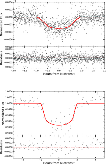
Figure 1. Phase-folded K2 transit light curves of K2-106b (top) and K2-106c (bottom). The dark points show the measurements and the red lines show the best-fit model, with residuals plotted below the light curves.
Download figure:
Standard image High-resolution imageK2-106 was observed by TESS between 2021 August 20 and September 16, in Sector 42 by camera 3 in cycle 4. The TESS data was processed through the TESS Science Processing Operations Center (SPOC) pipeline, and the light curve was retrieved via the Barbara A. Mikulski Archive for Space Telescopes (MAST). We removed any data points that were flagged for quality issues. We detrended the light curve using Wōtan before conducting a transit search using transit least squares. The search produced a planet detection with a signal-to-noise ratio (S/N) of ∼3. Thus, the TESS light curve for K2-106 does not provide any useful additional constraints and therefore we did not use it in this work.
2.2. Radial Velocities
G17 determined that K2-106 is inactive based on their derivation of an average chromospheric activity index of log  , which is near the minimum value of the chromospheric activity index for stars with solar metallicity (∼log
  ). They also and derive a slow rotation for the star of
  km s−1, thus concluding that the star is inactive.
To constrain the masses of K2-106b and K2-106c, we used multiple RV data sets collected by G17 as well as HIRES RV data from Sinukoff et al. (2017). We briefly describe the instruments and the data below.
PFS. We used 13 spectra of K2-106 from the Carnegie Planet Finder Spectrograph (PFS; Crane et al. 2006, 2010) on the 6.5 m Magellan/Clay Telescope, taken between 2016 August 14 and 2017 January 14. PFS has a resolving power of λ/Δλ ∼ 76,000. The exposures ranged from 20 to 40 minutes and had an S/N of 50–140 per pixel. The relative velocities were extracted from the spectrum using the techniques in Butler et al. (1996).
HDS. We used three RV measurements from the High Dispersion Spectrograph (HDS; Noguchi et al. 2002) located on the 8.2 m Subaru Telescope, obtained between 2016 October 12 and 14. The telescope has a resolving power of λ/Δλ ∼ 85,000 and a typical S/N of 70–80 per pixel. G17 notes that, as with PFS, the HDS RVs were measured relative to a template spectrum taken by the same instrument without the iodine cell.
FIES. We used six RV measurements from the FIbre-fed Echelle Spectrograph (FIES; Frandsen & Lindberg 1999; Telting et al. 2014) on the 2.56 m Nordic Optical Telescope (NOT) at the Observatorio del Roque de los Muchachos, in La Palma, Spain. The observations were taken from 2016 October 5 to November 25. They used the 1 3 high-resolution fiber, with λ/Δλ ∼ 67,000, and they reduced the spectra using standard IRAF and IDL routines.
HIRES. We included 35 RV measurements taken by Sinukoff et al. (2017) from the HIRES instrument at Keck (Vogt et al. 1994), which has a resolving power of ∼55,000.
HARPS and HARPS-N. We used 20 RV measurements from the High Accuracy Radial velocity Planet Searcher (HARPS; Mayor et al. 2003) spectrograph on the 3.6 m ESO Telescope at La Silla, Chile. Additionally, we used 12 RV measurements from the HARPS-N instrument at the 3.58 m Telescopio Nazionale Galileo (TNG) at La Palma (Cosentino et al. 2012). The HARPS spectra were obtained from 2016 October 25 to 2016 November 27 and the HARPS-N data between 2016 October 30 and 2017 January 28. Both instruments have a resolving power of λ/Δλ ∼ 115,000. The spectra were then reduced with the dedicated HARPS and HARPS-N pipelines.
In total, we used 89 RV measurements for our analysis. We refer the reader to G17 and Sinukoff et al. (2017) for more detailed descriptions of all the RV measurements and their reductions. The phase-folded RV curves of the system are plotted in Figure 2

Figure 2. Phase-folded RV measurements of K2-106b (top) and K2-106 c (bottom). The red line shows the best-fit EXOFASTv2 model, with residuals plotted below the RV curves. TP is the time of periastron, while TC is the time of conjunction or transit.
Download figure:
Standard image High-resolution image3. Methods
3.1. EXOFASTv2 Global Fits
To constrain the K2-106 system parameters, we performed a global fit of the K2 photometry and RV data with the publicly available exoplanet-fitting software EXOFASTv2 (Eastman et al. 2013; Eastman 2017; Eastman et al. 2019). EXOFASTv2 can fit multiple light curves and RV data sets and can model single- and multi-planet systems using a differential evolution Markov Chain Monte Carlo (MCMC) algorithm.
We determined the host star properties by fitting the star's spectral energy distribution (SED) simultaneously with the RV and photometric data using available broadband photometry, specifically Gaia G, GBP, and GRP; Two Micron All Sky Survey (2MASS) JHK magnitudes, and Wide-field Infrared Survey Explorer (WISE) W1-W4 magnitudes; these are all given in Table 1. We adopted a parallax of μ = 4.085 ± 0.018 mas from Gaia EDR3. The fluxes were fit using the Kurucz (1992) atmosphere models. We set a prior on the maximum line-of-sight visual extinction AV of 0.17 from the maps of Schlegel et al. (1998). We also adopted a wide [Fe/H] metallicity prior of =0.06 ± 0.2 dex. This central value is the median of the metallicities reported in the literature for K2-106. The SED fit is shown in Figure 3. For a detailed description of the stellar SED fitting with EXOFASTv2, see, e.g., Godoy-Rivera et al. (2021).
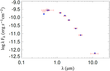
Figure 3. Spectral Energy Distribution of K2-106. The red crosses show the broadband observations and the error bars show the width of the filters. The blue circles represent the model fluxes.
Download figure:
Standard image High-resolution imageUsing the resulting stellar properties from the SED fit as priors, we then performed a global fit of the system, using the K2 photometry and the six RV data sets described in Section 2. We adopted an initial guess on the ephemerides of planets b and c from G17 of Tb = 2457394.0114 BJDTDB and Tc = 2457405.7315 BJDTDB, and on their orbital periods of Pb = 0.57 days and Pc = 13.33 days, respectively. We assumed a zero eccentricity for K2-106b, which we justify as follows. The tidal circularization timescale, τcirc, for a planet of mass, Mp , radius, Rp , semimajor axis, a, and tidal quality factor, Q, is given by
(Goldreich & Soter 1966). The tidal quality factor Q for exoplanets is highly uncertain but we adopt a value of Q = 100, which is reasonable for rocky planets (e.g., Henning et al. 2009). Using the mass and radius from G17, we derive a tidal circularization timescale of τcirc ≤ 10,000 yr. Given the age that we infer for this system of  Gyr, we deduce that enough time has passed for the planet's orbit to have been completely circularized, thus justifying our assumption that e = 0. We do not make the same assumption for K2-106c, however, given its longer orbital period of ∼13 days. We impose a prior of e = 0 ± 0.2 per Eylen et al. (2019), who measured eccentricities of singly and multiply transiting planets and found that the singles can be described by a Gaussian with a dispersion of σe
= 0.32 ± 0.06 and the multiples with
Gyr, we deduce that enough time has passed for the planet's orbit to have been completely circularized, thus justifying our assumption that e = 0. We do not make the same assumption for K2-106c, however, given its longer orbital period of ∼13 days. We impose a prior of e = 0 ± 0.2 per Eylen et al. (2019), who measured eccentricities of singly and multiply transiting planets and found that the singles can be described by a Gaussian with a dispersion of σe
= 0.32 ± 0.06 and the multiples with  .
.
We performed two global fits of the system: one using constraints from the MIST stellar evolutionary models and another without any constraints from stellar evolutionary models. The results of both analyses are shown in Tables 2 (with constraints from MIST) and 3 (without) and are discussed in Section 4. The stellar and planetary parameters we derived for both the MIST and the model-independent fits are consistent with each other, as shown in Tables 4 (stellar parameters) and 5 (planetary parameters).
Table 2. Median Values and the 68% Confidence Interval for the Physical Parameters of K2-106b and K2-106c from the Global Fit Using Constraints from MIST
| Parameter | Description (Units) | Values | Values | ||
|---|---|---|---|---|---|
| K2-106b | K2-106 c | ||||
| P | Period (days) |

|

| ||
| RP | Radius (R⊕) |

|

| ||
| MP | Mass (M⊕) | 8.53 ± 1.02 |

| ||
| TC | Time of conjunction (BJDTDB) | 2457394.0106 ± 0.0013 |
| ||
| a | Semimajor axis (au) |

|

| ||
| i | Inclination (degrees) |

|

| ||
| Teq | Equilibrium temperature (K) |

|

| ||
| K⋆ | RV semiamplitude (m s−1) |

|

| ||
| RP /R* | Radius of planet in stellar radii |

|

| ||
| a/R* | Semimajor axis in stellar radii |

|

| ||
| δ | Transit depth (fraction) |

|

| ||
| τ | Ingress/egress transit duration (days) |

|

| ||
| e | Eccentricity | 0 (fixed) |

| ||
| T14 | Total transit duration (days) |

| 0.1498 ± 0.0047 | ||
| TFWHM | FWHM transit duration (days) |

|

| ||
| b | Transit impact parameter |

|

| ||
| ρP | Density (cgs) |

|

| ||
| loggP | Surface gravity |

|

| ||
| Θ | Safronov number | 0.00484 ± 0.00057 |

| ||
| 〈F〉 | Incident flux (109 erg s−1 cm−2) |

|

| ||
| TS | Time of eclipse (BJDTDB) | 2457394.2962 ± 0.0013 |

| ||
| TA | Time of ascending node (BJDTDB) | 2457394.4391 ± 0.0013 |

| ||
| TD | Time of descending node (BJDTDB) | 2457394.1534 ± 0.0013 |

| ||

| Minimum mass (M⊕) | 8.497 ± 1.01 |

| ||
| MP /M* | Mass ratio | 0.0000266 ± 0.0000031 |

| ||
| d/R* | Separation at mid-transit |

|

| ||
| PT | A priori nongrazing transit prob |

|

| ||
| PT,G | A priori transit prob |

|

|
Download table as: ASCIITypeset image
Table 3. Median Values and the 68% Confidence Interval for the Physical Parameters of K2-106b and K2-106c from the Model-independent Global Fit
| Parameter | Description (Units) | Values | Values | ||
|---|---|---|---|---|---|
| K2-106b | K2-106 c | ||||
| P | Period (days) |

| 13.3393 ± 0.0015 | ||
| RP | Radius (R⊕) |

|

| ||
| MP | Mass (M⊕) |

|

| ||
| TC | Time of conjunction (BJDTDB) | 2457394.0106 ± 0.0013 |
| ||
| a | Semimajor axis (au) |

|

| ||
| i | Inclination (degrees) |

|

| ||
| e | eccentricity (degrees) | 0 (fixed) |

| ||
| Teq | Equilibrium temperature (K) |

|

| ||
| K⋆ | RV semiamplitude (m s−) | 6.68 ± 0.75 |

| ||
| RP /R* | Radius of planet in stellar radii |

|

| ||
| a/R* | Semimajor axis in stellar radii |

|

| ||
| δ | Transit depth (fraction) |

|

| ||
| τ | Ingress/egress transit duration (days) |

|

| ||
| T14 | Total transit duration (days) |

| 0.1498 ± 0.0047 | ||
| TFWHM | FWHM transit duration (days) |

|

| ||
| b | Transit impact parameter |

|

| ||
| ρP | Density (cgs) |

|

| ||
| loggP | Surface gravity |

|

| ||
| Θ | Safronov number |

|

| ||
| 〈F〉 | Incident flux (109 erg s−1 cm−2) |

|

| ||
| TS | Time of eclipse (BJDTDB) | 2457394.2962 ± 0.0013 |

| ||
| TA | Time of ascending node (BJDTDB) | 2457394.4391 ± 0.0013 |

| ||
| TD | Time of descending node (BJDTDB) | 2457394.1534 ± 0.0013 |

| ||

| Minimum mass (M⊕) |

|

| ||
| MP /M* | Mass ratio |

|

| ||
| d/R* | Separation at mid-transit |

|

| ||
| PT | A priori nongrazing transit prob |

|

| ||
| PT,G | A priori transit prob |

|

|
Download table as: ASCIITypeset image
Table 4. Stellar Properties
| Reference | Teff |

| M⋆ | R⋆ | ρ⋆ | [Fe/H] |
|---|---|---|---|---|---|---|
| (K) | (M⊙) | (R⊙) | (g/cm3) | (dex) | ||
| This work (no models) |

|

|

|

|

| −0.03 ± 0.01 a |
| This work (MIST) | 5508 ± 70 |

|

|

| 1.46 ± 0.14 | −0.03 ± 0.01 a |
| Adams et al. (2017) | 5590 ± 51 | 4.56 ± 0.09 | 0.93 ± 0.01 | 0.83 ± 0.04 | ⋯ | 0.02 ± 0.02 |
| Sinukoff et al. (2017) | 5496 ± 46 | 4.42 ± 0.05 | 0.92 ± 0.03 | 0.95 ± 0.05 | ⋯ | 0.06 ± 0.03 |
| Guenther et al. (2017) | 5470 ± 30 | 4.53 ± 0.08 | 0.94 ± 0.06 | 0.87 ± 0.08 | ⋯ | -0.02 ± 0.05 |
| Dai et al. (2019) | 5496 ± 46 | 4.42 ± 0.05 |

|

|

| 0.06 ± 0.03 |
Note. Adams et al. (2017), Sinukoff et al. (2017), and Guenther et al. (2017) report M⋆ and R⋆, but do not report a stellar density ρ⋆. We do not compute a stellar density from their masses and radii since the uncertainties in the latter are correlated.
a This metallicity value was measured using a high-resolution spectrum (see Section 5.1), but we also infer an [Fe/H] abundance using the global fit with MIST constraints. These sets of abundances are consistent within their uncertainties but we adopt the more precise spectroscopic [Fe/H].Download table as: ASCIITypeset image
Table 5. Planet Properties
| Reference | Period | K⋆ | Rp /R⋆ | Rp | Mp | ρp | CMFρ |
|---|---|---|---|---|---|---|---|
| (days) | (m s−1) | (R⊕) | (M⊕) | (g/cm3) | (%) | ||
| This work (no models) |

| 6.68 ± 0.75 |

|

|

|

|

|
| This work (MIST) |

|

|

|

| 8.53 ± 1.02 |

|

|
| Adams et al. (2017) | 0.571308 ± 0.000030 | ⋯ |

| 1.46 ± 0.14 | ⋯ | ⋯ | ⋯ |
| Sinukoff et al. (2017) | 0.571336 ± 0.000020 | 7.2 ± 1.3 |

|

|

| ⋯ | |
| Guenther et al. (2017) |

| 6.67 ± 0.69 |

| 1.52 ± 0.16 |

|

|

|
| Dai et al. (2019) | 0.571 |

|

| 1.71 ± 0.07 |

| 8.5 ± 1.90 | 40 ± 23 |
Download table as: ASCIITypeset image
4. Results
We first discuss the fit we performed without external constraints from stellar models. In order to break the well-known M⋆ − R⋆ degeneracy in the fits of transiting planets (Seager & Mallen-Ornelas 2003), we fit the star's SED using broadband photometry from publicly available all-sky catalogs combined with the Gaia EDR3 parallax to provide a constraint on R⋆ (see Section 3.1). For this fit, we obtain a stellar mass of  , a radius of
  , a stellar effective temperature of
  K, and a density of
  g cm−3. We derive a stellar mass and RV semiamplitude K⋆ consistent with G17, but derive a larger value for the stellar radius, leading to a planetary density of
  g cm−3 (with a ∼25% uncertainty), which is lower than that derived by G17 of
  g cm−3, but still consistent to within 1σ. We conclude that, in agreement with the predictions from Rodriguez Martinez et al. (2021), an analysis using purely empirical constraints on R⋆ and M⋆ results in a tighter constraint on the planetary density.
We subsequently modeled the system additionally using priors on the host star from the MIST stellar evolutionary tracks and obtained consistent central values of the stellar and planetary parameters, but with slightly lower uncertainties than those derived from the fit without external constraints, as expected. From this fit, we obtain a planetary density of  g cm−3, which is only slightly higher than, but consistent with, the one we derive without using MIST. We derive a stellar effective temperature of Teff = 5508 ± 70 K and an isochronal age of
  Gyr. The temperature from both fits indicate that K2-106 is a late-type G star, either G7 or G8, based on the classifications of Pecaut & Mamajek (2013). Both temperatures lead to a high equilibrium temperature for K2-106b of
  K (from the model-independent fit) and
  K (from the MIST fit).
Our analysis of K2-106b indicates that although it is highly dense and possibly an iron-enriched relative to Earth, it may not be a super-Mercury. Figure 4 shows the mass and radius measurements of K2-106b and K2-106c, with other values from the literature plotted for reference. As can be seen from the plot, the measurement from G17 places K2-106b below the Mercury-like composition curve, implying an iron mass fraction possibly higher than that of Mercury (of ∼70%). The masses and radii from both Sinukoff et al. (2017) and Dai et al. (2019) imply a lower density and thus a more Earth-like composition.
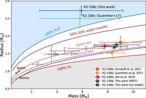
Figure 4. Mass–radius diagram highlighting the measurements of K2-106b and K2-106c from this work and from previous literature. The colored lines are theoretical mass–radius curves from Zeng et al. (2019). Planets below the black dashed line would exceed the maximum iron allowed from collisional mantle stripping computed by Marcus et al. (2010). The gray points show the masses and radii of several other USPs for reference. Earth and Venus are also plotted for reference.
Download figure:
Standard image High-resolution imageFigure 5 shows the mass and density distribution of planets with Rp
< 2 R⊕ and Mp
< 10 M⊕.
5
These planets have an average bulk density of 6.59 g cm−3. With a density of  g cm−3 (1.7ρ⊕), K2-106b ranks among the densest worlds known and is denser than 91% of such planets. Also notable in Figure 5 is a trend in density with equilibrium temperature: the denser, potentially rocky exoplanets (ρp
/ρ⊕ > 1) are generally hotter than lighter volatile-rich planets. This apparent dichotomy in bulk density as a function of equilibrium temperature (or semimajor axis) is consistent with the photoevaporation of H/He envelopes for the hottest planets (e.g., Owen & Wu 2017). This trend may also support the theory that the densest planets form in the inner regions of the protoplanetary disk, where there is a greater supply of iron relative to other refractory elements (see, e.g., Wurm et al. 2013).
g cm−3 (1.7ρ⊕), K2-106b ranks among the densest worlds known and is denser than 91% of such planets. Also notable in Figure 5 is a trend in density with equilibrium temperature: the denser, potentially rocky exoplanets (ρp
/ρ⊕ > 1) are generally hotter than lighter volatile-rich planets. This apparent dichotomy in bulk density as a function of equilibrium temperature (or semimajor axis) is consistent with the photoevaporation of H/He envelopes for the hottest planets (e.g., Owen & Wu 2017). This trend may also support the theory that the densest planets form in the inner regions of the protoplanetary disk, where there is a greater supply of iron relative to other refractory elements (see, e.g., Wurm et al. 2013).
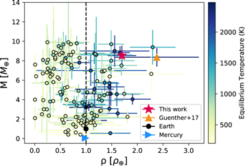
Figure 5. Mass as a function of bulk density (normalized by the values of Earth) for known planets with Mp < 10 M⊕. The dashed vertical line represents a constant Earth-like density. K2-106b is shown by a pink star, while the golden triangle is the value from Guenther et al. (2017). The points are color coded by their equilibrium temperature. Earth and Mercury are overplotted for reference (the black circle and blue triangle, respectively).
Download figure:
Standard image High-resolution image5. Composition of K2-106b
The relative abundances of the refractory elements (such as Fe, Mg, and Si) in the Sun have been shown to closely match those of Venus, Earth, and chondrite meteorites in the solar system (Lodders et al. 2009). Many studies have since found strong chemical links between the relative abundances of the common, rock-forming elements Fe, Mg, and Si of the parent star and the compositions of their orbiting planets (see, e.g., Dorn et al. 2015; Brugger et al. 2017; Liu et al. 2020; Plotnykov & Valencia 2020; Adibekyan et al. 2021; Schulze et al. 2021; Wilson 2021). For example, Adibekyan et al. (2021) found a positive correlation between the density of rocky planets and the iron mass fraction of their parent stars. Thus, the refractory elemental abundances of host stars can be used as a proxy for the bulk composition and to constrain some properties of a planet's interior, such as the core/mantle mass and radius fractions. This is especially important because a planet's bulk density is degenerate with its interior composition.
One of the most important properties that characterizes the interior of a planet is its CMF, defined as the mass of the core divided by the total mass of the planet. The CMF is a first-order approximation of its composition and a factor in the existence and lifetime of a magnetic field. The latter, in turn, is an essential ingredient for habitability, as it shields the planet from high-energy charged particles and reduces atmospheric loss. To constrain the CMF and interior structure of K2-106b, we combine the planet's physical properties with the star's atmospheric Fe/Mg and Si/Mg abundances. We follow the statistical framework of Schulze et al. (2021), which we briefly summarize here and direct the reader to for a more in-depth description.
Schulze et al. (2021) calculate the CMF in two ways for approximately a dozen well-characterized short period planets with Rp < 2R⊕ and Mp < 10M⊕. First, they calculate the CMF expected from the planet's mass and radius, denoted as CMFρ . Then they calculate the CMF as predicted from the refractory elemental composition of the photosphere of the host star, denoted as CMF⋆ (and defined in Equation (2)). They then calculate the probability that a planet satisfies the null hypothesis H0, which says that the planet's composition reflects the chemical composition of its host star. This probability is denoted as P(H0), and is quantified by the amount of overlap between the probability distributions of CMFρ and CMF⋆. In their framework, if P(CMFρ = CMF⋆) ≤32%, then the planet deviates from the expected composition at the 1σ significance level, and if P(CMFρ = CMF⋆) ≤5%, then it deviates from the composition expected from the host star at the 2σ significance level.
Here, CMF⋆ is mathematically defined as
where X/Y are the stellar molar ratios for elements X and Y, and mi is the molar mass of species i. The uncertainty in CMF⋆ can be derived by propagating the uncertainties in Fe/Mg and Si/Mg; see Equation (3) of Schulze et al. (2021).
In the following subsections, we describe the chemical abundance determinations for K2-106 and the derivation of CMFρ and CMF⋆.
5.1. Stellar Abundance Measurements
An estimate of CMF⋆ requires [Fe/H], [Si/H], and [Mg/H] abundances. We computed these using an archival optical HARPS spectrum spanning a wavelength range between 450 and 691 nm. We used the framework for spectral analysis, iSpec (Blanco-Cuaresma et al. 2014; Blanco-Cuaresma 2019), which calculates stellar atmospheric parameters as well as individual abundances using both the synthetic spectral fitting method and the equivalent width (EW) method. Within iSpec we used the radiative transfer code SPECTRUM (Gray & Corbally 1994), the solar abundances from Grevesse et al. (2007), the MARCS.GES model atmospheres (Gustafsson et al. 2008), and the atomic line list from the Gaia–ESO Survey (GES), which covers the entire wavelength of our spectrum.
To constrain the chemical abundances and their uncertainties via the spectral fitting method, we first calculated the spectrum's S/N with iSpec, which yielded an S/N ∼ 37, with which we estimated the spectrum errors. We first derived the stellar atmospheric parameters with iSpec using the synthetic spectral fitting method. We fixed the projected stellar rotation,  , to 2 km s−1 and the limb-darkening coefficient to 0.6 to avoid possible degeneracies between the macroturbulence and rotation, following the recommendations of Blanco-Cuaresma et al. (2014). We derive the following parameters: Teff = 5543.5 ± 27.9 K,
  , [M/H] = −0.01 ± 0.02 dex, α = 0.1 ± 0.02, a microturbulent velocity of vmic = 1.54 ± 0.05 km s−1, and a macroturbulent velocity of vmac = 3.58 ± 0.12 km s−1. To calculate the Fe, Mg, and Si abundances, we fixed all the stellar parameters to the values spectroscopically determined with iSpec and only let the abundances vary. We opted to use the spectroscopic stellar parameters instead of the parameters derived from EXOFASTv2 because this ensures that both stellar parameters and abundances are calculated self-consistently. We note, however, that the stellar parameters derived with iSpec and EXOFASTv2 are consistent within their uncertainties.
To account for systematics in the abundance determinations, we calculated the total uncertainty in each abundance as the quadrature sum of the uncertainties from the iSpec errors and the contribution from atmospheric parameters Teff,  , and [M/H]. To estimate the systematic uncertainty from the atmospheric parameters, we performed a series of runs in which we fixed each stellar parameter (Teff,
  , and [M/H]) to its −2σ, −1σ, 1σ, and 2σ values and calculated the [X/H] abundance at each value while fixing the other stellar parameters to their central values. Then, the systematic error in abundance from each stellar parameter was calculated as the deviation in the 2σ abundances from their central values, divided by 2. Our final abundances are [Fe/H] = −0.03 ±0.01, [Mg/H] = 0.04 ± 0.02, and [Si/H] = 0.03 ± 0.06. To validate our measurements, we also calculated the Fe, Mg, and Si abundances with the code MOOG (Sneden et al. 2012), which uses the equivalent width method, and obtained consistent sets of abundances. While writing this paper we noticed that another group, Adibekyan et al. (2021), derived abundances of K2-106. We considered their results for the analysis of the composition of K2-106b, but we ultimately adopt the abundances from this work. Adibekyan et al. (2021) used a high-resolution HARPS spectrum of K2-106 and the code MOOG to determine stellar abundances and obtained consistent [Mg/H] and [Si/H] abundances but slightly higher [Fe/H] than we do (see Table 6).
Table 6. Abundance Measurements
| Source | [Fe/H] | [Mg/H] | [Si/H] | Si/Mg | Fe/Mg | CMF⋆ |
|---|---|---|---|---|---|---|
| This work (iSpec) | −0.03 ± 0.01 | 0.04 ± 0.02 | 0.03 ± 0.06 | 0.93 ± 0.25 | 0.71 ± 0.17 | 0.29 ± 0.06 |
| This work (MOOG) | −0.03 ± 0.01 | 0.03 ± 0.02 | 0.03 ± 0.04 | 0.95 ± 0.24 | 0.72 ± 0.18 | 0.29 ± 0.06 |
| Adibekyan et al. (2021) | 0.10 ± 0.03 | 0.07 ± 0.05 | 0.05 ± 0.03 | 0.78 ± 0.14 | 0.85 ± 0.16 | 0.35 ± 0.05 |
Download table as: ASCIITypeset image
5.2. Determination of CMFρ and CMF⋆
We calculated the stellar molar ratios Fe/Mg and Si/Mg using Equation (5) from Hinkel & Unterborn (2018) and the associated uncertainties by propagating the errors from the abundance measurements. We calculate these ratios for three sets of abundance measurements: (1) the abundances derived in this work using iSpec, (2) the abundances from MOOG, and (3) the abundances from Adibekyan et al. (2021). To determine CMF⋆, we insert the molar ratios in Equation (2). The abundances, molar ratios, and values of CMF⋆ are all listed in Table 6. All three abundance measurements lead to consistent values of CMF⋆ within the uncertainties.
We calculated CMFρ
using the ExoPlex program (Unterborn et al. 2018, 2022; Unterborn & Panero 2019), which self-consistently solves the equations of planetary structure including the conservation of mass, hydrostatic equilibrium, and the equation of state. The calculation of CMFρ
assumes a pure, liquid iron core and a magnesium silicate (MgSiO3) mantle free of iron. This calculation takes the planetary mass and radius as inputs and take their uncertainties as priors, as well as an initial guess for the CMFρ
of the planet. We calculate two values of CMFρ
. Using the planetary parameters from our model-independent fit, we get CMFρ
 . Using the parameters from the fit with MIST, we get a slightly higher value of CMFρ
 as expected, since the planet density inferred from MIST is higher.
To complement the CMFρ values from ExoPlex, we calculate the core-radius fraction (CRF) for K2-106b using the python package HARDCORE (Suissa et al. 2018), which uses boundary conditions to bracket the minimum and maximum CRF for a rocky planet, assuming a fully differentiated planet and a solid iron core. Once the CRF is known, the CMF can be approximated by CMF ≈ CRF2 (Zeng & Jacobsen 2017). For the planetary parameters from the empirical fit, we obtain a CRF of 64% ± 17%, which corresponds to a CMF of 40% ± 21%. Using the planetary parameters from the fit with MIST, we obtain a CRF of 68% ± 11%, corresponding to a CMF of 46% ± 15%, both of which are fully consistent with the values from ExoPlex.
5.3. Is K2-106b Mercurified?
We find a value of P(H0) = 56.6% for the CMFρ and CMF⋆ calculated in this work, and P(H0) = 76.1% for the CMF⋆ and CMFρ from the planetary mass and radius and stellar abundances from Adibekyan et al. (2021). Based on our formalism, only planets for which P(CMFρ = CMF⋆) ≤32% deviate from the composition expected from the host star at the 1σ significance level. Thus, our values of P(H0) = 56.6% and P(H0) = 76.1% imply that K2-106b is entirely consistent with its host star's chemical composition. Figure 6(a) shows the effect of correlating the planet's mass and radius via the surface gravity. As demonstrated in Rodriguez Martinez et al. (2021), the constraint on the planet's surface gravity improves the precision on the planet's CMF, as shown by the green ellipses. Figure 6(b) shows the probability distribution functions and the overlap between CMFρ and CMF⋆. Both stellar abundances and planetary parameters from this work or from Adibekyan et al. (2021) lead to the conclusion that K2‐106b is decisively Earth‐like and does not have a Mercury‐like composition. We conclude that the lower stellar radius and thus the lower planetary radius derived by previous authors led this planet to be misidentified as a super-Mercury in the literature. This highlights the importance of including the improved constraint on R⋆, which is due to the more precise Gaia DR3 parallax. It is worth pointing out, however, that some of the previous authors who analyzed the K2-106 system, including G17, did not have access to Gaia DR2, and instead used the much lower-precision parallax from the Tycho–Gaia Astrometric Solution (TGAS; Michalik et al. 2015).

Figure 6. Left: 1σ and 2σ mass–radius ellipses for K2-106b. The violet ellipses assume that Mp and Rp are uncorrelated variables. The green ellipses represent the 1σ and 2σ errors when Mp and Rp are correlated via the planetary surface gravity, gp . Planets along the blue, red, and black solid lines follow a CMFρ of 0.29, 0.35, and 0.44, respectively. The added constraint of gp reduces the uncertainty in the CMF. Right: 1σ distributions of the probability density functions (PDF) of the iron mass fraction or CMF⋆ for the abundances derived in this work (cyan) and for the Adibekyan et al. (2021) values (red), and CMFρ outlined in purple (for uncorrelated Mp and Rp ) and green (for correlated).
Download figure:
Standard image High-resolution image5.4. Composition Models of Acuña et al. (2021)
We complement the compositional analysis described in the previous section with the models from Acuña et al. (2021), which follow an MCMC Bayesian algorithm (Director et al. 2017; Acuña et al. 2021). The planet's interior is modeled with three layers: an Fe core, a Si-dominated mantle, and a hydrosphere in steam and supercritical states (Mousis et al. 2020; Acuña et al. 2021). When a water-dominated atmosphere is present, we compute its emitted radiation and Bond albedo to determine radiative–convective equilibrium with a 1D k-correlated model (Pluriel et al. 2019, Acuña et al. in prep). The composition is therefore parameterized by two variables: the CMF and the water mass fraction (WMF). In our MCMC Bayesian analysis, the observables are the planetary mass and radius, and optionally the Fe/Si molar ratio. We consider three scenarios: in scenario 1, we assume that K2-106b is a completely dry planet (WMF = 0), while the CMF is the only free non-observable parameter, and the mass and the radius are the observables. Scenario 2 is similar to scenario 1, but now the WMF is no longer constant and it is left as a free parameter. Finally, in scenario 3, we include and treat the Fe/Si ratio as an observable. Its mean value and uncertainties are calculated from the host stellar abundances (see Table 6). The resulting value is Fe/Si = 0.672 ± 0.094. The output of our interior Bayesian analysis are the posterior distributions of the compositional parameters (CMF and WMF) and the observables (mass, radius, and Fe/Si), which are shown in Table 7.
Table 7. MCMC Parameters of the Interior Structure Analysis and Their 1σ Confidence Intervals for All Three Scenarios
| Parameter | Scenario 1 | Scenario 2 | Scenario 3 |
|---|---|---|---|
| CMF |

|

| 0.24 ± 0.03 |
| WMF | 0 | (5.8 ) 10−5 ) 10−5
| (9.8 ± 7.8) 10−5 |
| Mp [M⊕] |

|

|

|
| Rp [R⊕] |

|

|

|
| Fe/Si | 2.05 ± 1.52 | 4.75 ± 5.27 | 0.71 ± 0.11 |
Note. In scenarios 1 and 2, our Bayesian model reproduces a CMF, Mp , and Rp that are consistent with the results from our analysis in Section 5.2. However, the model's retrieved CMF, mass, and radius in scenario 3 do not reproduce well the observed values.
Download table as: ASCIITypeset image
In scenario 1, the retrieved CMF is compatible with the estimates based on our approach from Section 5.2 of CMF =  . The planet's mass and radius are also reproduced by the model within their uncertainties. The 1σ confidence intervals obtained by both interior models overlap with the interval of 23%–35% for CMF⋆. We also explore if the estimated CMF by our model, assuming the presence of an atmosphere, is compatible with that of the star.
In scenario 2, the mean value of the CMF is higher than the CMF in scenario 1, but both are compatible within the uncertainties. In this scenario, the observed planetary mass and radius are also well reproduced by the model. A slightly higher CMF in scenario 2 is necessary to reproduce the observed mass and radius since a more Fe-rich bulk is more dense, leaving more space for a low-density steam atmosphere to expand with respect to the dry scenario. As can be seen in Figure 7, the estimated CMF in scenario 2 is compatible within uncertainties with the CMF estimated in our scenario 1 and by our previous estimate, although it is not compatible with CMF⋆. This means that if K2-106b was to reflect the CMF estimated from the abundances of its host star, it would be very unlikely to have a thick steam atmosphere, or indeed any atmosphere with a mean molecular weight lower than 18. If an atmosphere exists, the CMF would have to be greater than 0.46, which is the lower limit of the 1σ confidence interval in scenario 2, and the atmosphere would have to be very thin. The properties of such a thin atmosphere would be Psurf = 184.9 ± 120.8 bar, zatm = 404 ± 82 km, Tsurf = 4154 ± 326 K, and AB = 0.210 ± 0.001 of the surface pressure, atmospheric scale height, surface temperature, and Bond albedo, respectively.
In scenario 3, the MCMC Bayesian analysis can reproduce the Fe/Si molar ratio derived from the host stellar abundances, but the mass and radius are not compatible with their observed mean values and uncertainties. The retrieved CMF in scenario 3 is compatible with CMF⋆, as expected, since both estimates are calculated from the chemical abundances of the host star. In scenario 3, the retrieved mass is lower than the observed value, whereas the retrieved radius is higher than the observed one, yielding a lower planetary density. This supports the conclusion we reached in scenario 2: K2-106b cannot have a steam atmosphere and reflect the refractory abundances of its host star simultaneously. Since any atmosphere with a lower mean molecular weight μ would have a higher scale height, we further conclude that K2-106b cannot have a substantial atmosphere with μ ≲ 18, which includes H- and He-dominated atmospheres.
5.5. Likelihood of a Substantial Atmosphere on K2-106b and K2-106c
In this section, we assess the probability that K2-106b and K2-106c have extended atmospheres from a different angle. Given both the high density ( g cm−3) and orbital period (P = 0.57 days) of K2-106b, it is probable that any primordial atmosphere it may have accreted during formation has been lost to atmospheric escape. We consider this possibility by estimating the XUV-driven mass-loss rate of the atmosphere over the planet's lifetime. First, we consider the restricted Jeans escape parameter Λ (Fossati et al. 2017), defined as

where mH is the mass of a hydrogen atom; Mp , Rp , and Teq are the mass, radius, and equilibrium temperature of the planet; and kB is Boltzmann's constant. We calculate a restricted Jean's escape value of 16.5 for K2-106b. Cubillos et al. (2017) found that planets with restricted Jean's escape parameters Λ ≤ 20 cannot retain hydrogen-dominated atmospheres and are in the boil-off"regime. Below this value, atmospheric escape is mainly driven by a combination of planetary thermal energy and low gravity rather than by high irradiation (Sanz-Forcada et al. 2011).
Next, we estimate the mass-loss rate  assuming that K2-106b formed with a substantial atmosphere and that the main driver of atmospheric escape is a combination of planetary intrinsic thermal energy and low gravity—using the following equation from Kubyshkina et al. (2018)

where the coefficients in the equation are determined by whether Λ is above or below a certain value and they are given in Kubyshkina et al. (2018). We estimate the XUV flux, FXUV, using the age–luminosity relations from Sanz-Forcada et al. (2011). For K2-106b, we expect  g s−1. Assuming that the initial mass of the atmosphere is 1% of the total mass of the planet, the atmosphere would be completely evaporated in ∼126 Myr. Given the current age of the system of ∼5.5 Gyr, K2-106b should have lost any primary atmosphere it may have had. This result agrees with the findings of Fossati et al. (2017) who predicted that planets with masses lower than 5M⊕, equilibrium temperatures higher than 1000 K, and Λ between 20 and 40 would have atmospheres that would evaporate in ≲500 Myr. Therefore, in agreement with Fossati et al. (2017) and G17, we posit that K2-106b is unlikely to have a substantial atmosphere.
For K2-106 c, we derive a density of  g cm−3 for the global fit with constraints from MIST and
  g cm−3 for the model-independent fit. The relatively low mass and bulk density of K2-106 c suggests that it could be a low-density super-Earth with an extended hydrogen atmosphere, or that it contains a substantial fraction of water (an ocean world; Kuchner 2003; Léger et al. 2004).
G17 estimated a mass-loss rate of  g s−1 and Λ = 28.8 ± 9.2. They concluded that, at its estimated atmospheric escape rate, K2-106c is likely in the boil-off regime and should have lost its atmosphere in a few megayears, similar to its hotter sibling. To rule out the possibility that K2-106c has a terrestrial composition, we estimate the mass and RV semiamplitude that K2-106c would have if it were purely rocky and compare them to the actual observed values. Assuming a density of 5 g cm−3, which is typical of the solar system rocky planets, we obtain a mass and an RV semiamplitude of 18.25M⊕ and Kc,rocky=5.01[C8] m s−1. However, this K* value is a 3.67σ discrepant from our derived value, which suggests that K2-106c is very unlikely to be rocky. Given the uncertainty in its mass, more observations will be needed to resolve the composition of K2-106c.
These conclusions may be tested with future follow-up atmospheric observations. Given its short period, K2-106b's orbit is likely to be circularized (as we show in Section 3.1) and also to be tidally locked to its host star. In the absence of an atmosphere, tidal locking would lead to high temperature contrasts between the dayside and the nightside, with differences between both sides of the order of 1000 K. Nevertheless, if K2-106b possesses an atmosphere, winds from the hot dayside could distribute the heat to the cool nightside and thus partially homogenize the planet's surface temperature. One way to confirm or rule out the presence of an atmosphere could be to obtain a phase curve of the planet with the James Webb Space Telescope (JWST). Recently, Kreidberg et al. (2019) obtained phase curves with Spitzer of the low-mass ultra-short-period planet LHS-3844b and derived a dayside temperature of 1040 ± 40 K and a temperature consistent with zero Kelvin on the nightside, ruling out the presence of an atmosphere on the planet. They reasoned that if LHS-3844b possessed a substantial atmosphere, it could distribute the heat from the dayside to the nightside and thus we would not observe such a large day- and nightside temperature variation. They also modeled the emission spectra of several rocky surfaces and compared them to the planet-to-star flux they measure for the planet, and conclude that its reflectivity is most consistent with a basaltic composition, i.e., with a crust formed from volcanic eruptions. This is a possible indication that the planet is a so-called lava world, a hypothesized planet characterized by high dayside equilibrium temperatures (Teq between 2500 and 3000 K) and surfaces covered by molten lava. Given the density, period, and the fact that it is likely tidally locked, K2-106b may well be a lava planet, which could be investigated by replicating the analysis of Kreidberg et al. (2019) to indirectly infer the presence or lack of an atmosphere (see also Keles et al. 2022 and Zieba et al. 2022). Additionally, if K2-106b is indeed a lava world, then perhaps magma oceans could have led to the formation of a secondary atmosphere of heavy elements through outgassing of volatiles in the interior (see, e.g., Papuc & Davies 2008), or a mineral atmosphere comprised of Na, Mg, O, or Si, (see, e.g., Ito & Ikoma 2021). To quantify the potential for follow-up phase curve observations of K2-106 with JWST, we calculate the transmission spectroscopy metric (TSM) proposed by Kempton et al. (2018). We obtain a TSM of 12.2 and 25 for K2-106b and K2-106c, respectively. These values are well below 92, which is the cutoff value suggested by Kempton et al. (2018) for planets in that size range. Although this system is not ideal for follow-up observations with JWST to learn more about the atmosphere or surface of its transiting planets, we nevertheless encourage more observations of the K2-106 system in order to improve upon the masses of its known planets.
6. Conclusions
In this paper, we revisited the K2-106 system and improved upon the physical properties of its two known transiting exoplanets. We employed planet interior models to demonstrate that, even though K2-106b is iron-enriched based on its high density and relatively large CMF, it is indistinguishable from its host stars' Fe/Mg ratios given the observational constraints, which implies that it did not suffer the formation processes responsible for Mercury's large core. Given its mass, radius, and chemical abundances of the parent star, K2-106b is unlikely to be a super-Mercury, as was previously thought. In addition, its high bulk density and proximity to its host star implies that K2-106b probably lacks a primordial or even secondary atmosphere and could perhaps be a barren lava world. In contrast, the low density of the outer planet, K2-106c ( g cm−3), suggests that it is it likely a water world. These hypotheses could potentially be tested with future follow-up observations with JWST.
To robustly characterize the interior structure and composition of low-mass planets, we will need extremely precise masses and radii with uncertainties on the order of <10% and ∼2%. Reaching these precisions is often difficult even with extensive transit and RV observations, as evidenced by this work. In addition, planet mass and radius alone are not sufficient to determine the interior structure of a planet, as is well known, and thus the refractory elemental abundances of the host star are extremely useful as a proxy for planet composition. Based solely on its bulk density, one might incorrectly deduce that K2-106b is a super-Mercury. Yet, upon more careful analysis, and after considering the refractory elemental abundances of the host star, it is apparent that the composition of K2-106b is more Earth-like and is consistent with the photospheric abundances of its host star. One corollary of this study, then, is that perhaps other putative super-Mercuries in the literature may not be as iron-enhanced as they seem. The characterization of super-Mercuries, as well as highly irradiated ultra-short-period planets, is critical to constrain the frequency and compositional diversity of small planets, and we therefore encourage more observations of K2-106 and similar systems.
R.R.M. and B.S.G. were supported by the Thomas Jefferson Chair for Space Exploration endowment from The Ohio State University. R.R.M. thanks Joseph Rodriguez, Jason Eastman, and Tharindu Jayasinghe for valuable discussions throughout this project. J.W. acknowledges the support by the National Science Foundation under grant No. 2143400. We acknowledge the academic gift from Two Sigma Investments, LP, which partially supports this research. We thank the anonymous referee for providing excellent feedback that improved the quality of this paper. This research has made use of the NASA Exoplanet Archive, which is operated by the California Institute of Technology, under contract with the National Aeronautics and Space Administration under the Exoplanet Exploration Program. This work has made use of data from the European Space Agency (ESA) mission Gaia (https://www.cosmos.esa.int/gaia), processed by the Gaia Data Processing and Analysis Consortium (DPAC; https://www.cosmos.esa.int/web/gaia/dpac/consortium). Funding for the DPAC has been provided by national institutions, in particular the institutions participating in the Gaia Multilateral Agreement.
Software: EXOFASTv2 (Eastman et al. 2019), ExoPlex (Unterborn et al. 2018), Wōtan (Hippke et al. 2019), iSpec (Blanco-Cuaresma et al. 2014; Blanco-Cuaresma 2019), HARDCORE (Suissa et al. 2018), numpy (Harris et al. 2020).
Appendix
In this section we show the posterior distribution functions of the core mass fractions discussed in Section 5.4. We also show a mass-radius diagram for K2-106b illustrating the realizations of the MCMC for the three scenarios from Section 5.4.

Figure 7. Posterior distribution functions of the CMFs for the three scenarios presented in Section 5.4. The distributions for CMF⋆ and the CMF estimated by the interior model of Schulze et al. (2021) under the assumption of a dry planet, similar to our scenario 1, are shown for comparison.
Download figure:
Standard image High-resolution image