


Abstract
We present results of cloud catalogs of 12CO, 13CO, and C18O (J = 1–0) in a section of the third Galactic quadrant over (195° < l < 220°, ∣b∣ < 5°) from the Milky Way Imaging Scroll Painting project. The data were acquired with the PMO 13.7 m millimeter telescope with ∼50''angular resolution. We construct three molecular cloud catalogs containing information of 12CO, 13CO, and C18O from the position–position–velocity (PPV) data cubes. The 12CO cloud catalog contains 7069 samples identified based on the DBSCAN algorithm. We develop a new algorithm, the stacking bump algorithm, for identifying 13CO and C18O emission by searching for weak signals in the original spectra of 13CO and C18O within the boundary in PPV space defined by the 12CO cloud. Above the 2σ threshold level, we identified 1197 clouds having 13CO emission and 32 clouds having C18O emission. We test the stacking bump algorithm in the noise-only datacube and find that the 2σ threshold can effectively avoid the possibility of false detection generated by noise. The results proved that the new algorithm has high accuracy and completeness. Statistics of peak intensity, projected angular area, line width, and flux of the clouds show that the power-law indices obtained from different isotopic lines are close to each other.
Export citation and abstract BibTeX RIS

Original content from this work may be used under the terms of the Creative Commons Attribution 4.0 licence. Any further distribution of this work must maintain attribution to the author(s) and the title of the work, journal citation and DOI.
1. Introduction
CO is the most abundant interstellar molecule after H2 (van Dishoeck & Black 1988). With CO emission being detected for the first time in the Orion Nebula (Wilson et al. 1970), it has become the most important tracer to study molecular clouds (MCs). The CO radiation is stronger and easier to detect, and the distributions of molecular gas and the kinematic information of detected clouds can be revealed (Shu et al. 1987).
Its isotopologues 13CO and C18O (J = 1 − 0) are important column density tracers of MCs (Dame et al. 2001) by assuming local thermodynamic equilibrium (LTE; Pineda et al. 2008; Wilson et al. 2009; Pineda et al. 2010). Since CO and its isotopologues have different abundances and optical depths, they can therefore be used to effectively trace the regions of MCs at different densities.
Over the past several decades, breakthroughs have been made in our understanding of the physical and dynamic information of MCs thanks to many large MC surveys (Dame et al. 1987; Kawamura et al. 1998; Dame et al. 2001; Heyer et al. 2001). The increase in the number of MC samples is one of the important factors leading to these breakthroughs. For example, Roman-Duval et al. (2010) found a power-law correlation between MCs' radii and masses. The CO excitation temperature of MCs decreases away from the Galactic center based on the 580 MCs with 12CO and 13CO line emission detected in the University of Massachusetts−Stony Brook (UMSB) and Galactic Ring surveys (Jackson et al. 2006). Rice et al. (2016) measured Larson's first law and found that its power-law index is near 0.5 everywhere based on 1064 massive MCs detected in the all-Galaxy CO survey of Dame et al. (2001). Fujita et al. (2019) found possible evidence for a cloud−cloud collision as a trigger of massive star formations in a Spitzer bubble N4 (Liu et al. 2016) via the FOREST Unbiased Galactic plane Imaging survey with the Nobeyama 45 m telescope (FUGIN; Umemoto et al. 2017). Another possible evidence for a cloud−cloud collision was found by Torii et al. (2021) in Sh 2–48 (Sharpless 1959) using the FUGIN data.
Although these results help us to better understand MC information, MC samples are still insufficient, and more samples are needed to help us study MCs. Yuan et al. (2021) visually classify the morphologies of 18,190 MCs identified in the 12CO data, which is the counterpart of the present survey in the second Galactic quadrant, and Yuan et al. (2022) used three different methods to extract the 13CO gas structures within each 12CO cloud. In larger sample studies, some important statistics will be well revealed, such as flux correlations between different molecular tracers. In this paper, we will focus on constructing an MC catalog containing complete information of 12CO, 13CO, and C18O.
This paper is the first in a series of large-sample MC studies in the third quadrant of the Milky Way. It focus on the establishment of MC samples. The data information is described in Section 2. Section 3 shows how we establish MC samples and identify 13CO and C18O emission. Basic statistical information for the sample will be presented in Section 4. Results obtained by different algorithms will be discussed in Section 5.
2. Data Reduction
2.1. Data
The third Galactic quadrant (195° < l < 220°, ∣b∣ < 5°) is part of the Milky Way Imaging Scroll Painting (MWISP) project, which is a multiline Galactic plane survey in CO and its isotopic transitions. Since the MWISP survey has been described in Su et al. (2021), we will briefly introduce it here.
The J = 1 − 0 transition lines of 12CO, 13CO, and C18O were obtained with the PMO 13.7 m millimeter telescope at Delingha. The telescope was mapped using a 3 × 3 pixel Superconducting Spectroscopic Array Receiver (SSAR) that works in sideband separation mode and employs the fast Fourier transform spectrometer (FFTS; Yang et al. 2008; Shan et al. 2012). The angular resolution of the 13.7 m telescope is about 49'' for 12CO and 51'' for 13CO and C18O. Each unit area of 30' × 30' was mapped using the on-the-fly (OTF) observation mode. The OTF raw data were regridded into regular data cubes with 30'' × 30'' pixels. Finally, the datacube units were mosaicked into a large datacube. Figure 1 shows the spectral noise distribution of 12CO, 13CO, and C18O in the total 250 deg2 region. The mean noise σ is ∼0.45 K for 12CO and ∼0.25 K for 13CO and C18O. The spatial distribution of spectral noise (Figure 2) indicates that the noise level of the overall data does not change significantly throughout the region. The velocity resolution is about 0.16 km s−1 for 12CO and 0.17 km s−1 for 13CO and C18O.
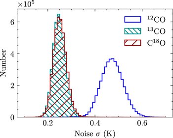
Figure 1. Spectral noise distribution of 12CO, 13CO, and C18O in the total 250 deg2 region.
Download figure:
Standard image High-resolution image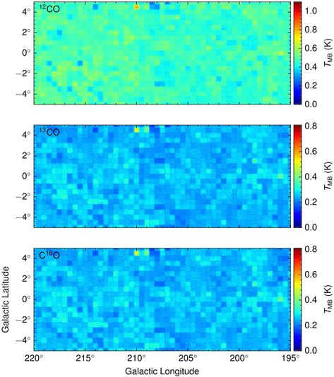
Figure 2. Spatial distribution of 12CO, 13CO, and C18O noise in the total 250 deg2 region.
Download figure:
Standard image High-resolution image2.2. CO Emission
Figure 3 presents integrated intensity maps of 12CO, 13CO, and C18O within the velocity range of [−20, 70] km s−1. We searched for the 12CO signal within [−200, 200] km s−1 and found it only in the range of [−20, 70] km s−1. The data covered a total area of 250 deg2, which contains some interesting and well-known MCs, star clusters, and nebulae, such as Mon OB1 (Lim et al. 2022), NGC 2264 (Herbig 1954), the Rosette Nebula (Schneider et al. 1998; Di Francesco et al. 2010), Maddalena (Maddalena & Thaddeus 1985), and Sh 2–287 (Sharpless 1959). Li et al. (2018) found evidence for a cloud−cloud collision in the Rosette Molecular Cloud, and the abundance ratios of 13CO to C18O in the cloud have a mean value of 13.7, which is 2.5 times larger than the solar system value (Wilson & Matteucci 1992). Su et al. (2017) present CO observations toward three large supernova remnants (SNRs; Green 2014), G205.5+0.5 (Monoceros Nebula; Xiao & Zhu 2012), G206.9+2.3 (PKS 0646+06; Gao et al. 2011), and G213.0+0.6 (Reich et al. 2003), in this region. Su et al. (2017) confirm that the two SNRs are physically associated with their ambient MCs, and they also find that the shock of SNRs is interacting with the molecular gas. Yan et al. (2019) calculated distances of 11 MCs using CO observations and the Gaia DR2 parallax and G-band extinction measurements in this region.
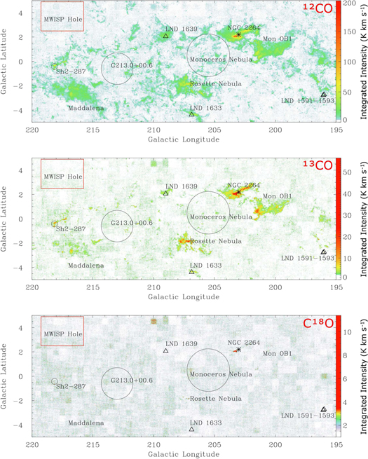
Figure 3. Integrated intensity map of 12CO, 13CO, and C18O within the velocity range of [−20, 70] km s−1. The intensity is integrated according to the 12CO cloud catalog boundary in PPV space that comes from the DBSCAN algorithm (Section 3.1). The circles symbolize SNRs (Green 2019) and H ii regions (for more information on H ii see Sharpless 1959; Anderson et al. 2014). The asterisk represents open cluster NGC 2264 (Herbig 1954). The triangles represent Lynds dark clouds (Lynds 1962). Some well-known MCs are also shown on the map. The newly discovered CO-dark hole (named "MWISP Hole") is marked with a rectangle in the upper left corner.
Download figure:
Standard image High-resolution imageThe 12CO emission shows the overall structure of the MC (Figure 3). It is noted that there is a large empty hole of no CO emission with an area of 8.4 deg2 (l = 217 5, b = 37' we named it the MWISP Hole) in the upper left corner. It is interesting that the MWISP Hole located in the Galactic disk with such low latitude and large size is quite rare. It also exists in the CO surveys of Dame et al. (1987). The strongest part of the 12CO emission is associated with NGC 2264. The 12CO intensity is mainly concentrated in the clouds Mon OB1, Rosette Nebula, and Maddalena, which are also the largest in the region.
Although the 13CO abundance is lower than that of the 12CO, this region still shows quite strong 13CO radiation. Its spatial distribution is similar to that of 12CO, and especially the clouds Mon OB1 and Rosette Nebula show a large area of spatial continuous structure. However, the emission of C18O is weak and it tends to be concentrated in a small dense core, so its radiation is not obvious on the large-scale spatial distribution map. We can see that the strongest C18O emission is in the cloud Mon OB1, but the radiation of other MCs is too weak and the spatial distribution scale is too small to be obvious.
Figure 4 presents the longitude–velocity map, which shows the velocity distribution of 12CO in this area. The figure clearly depicts the spiral arm structure in the third quadrant near the antigalactic center. The central velocities of 12CO emission in different spiral arms are systematically increased with the galactic longitude. The structure of spiral arms in the region will be discussed in detail in the future. A bright stripe exists at the velocity of 34.2 km s−1, which is caused by bad channels in the 12CO spectra. However, the bad channels do not exist in the 13CO and C18O spectra. The bad channel may affect identification and statistics of MCs, so we address this issue in Section 3.1.
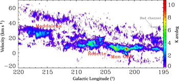
Figure 4. Longitude–velocity map of 12CO emissions. The latitude integration range is between −525 and 525. There is a bright stripe along the Galactic longitude in the figure, which is caused by a bad channel at the velocity of 34 km s−1.
Download figure:
Standard image High-resolution image3. Catalog
3.1. 12CO Cloud Catalog
Yan et al. (2020) investigated the decomposition of the 12CO spectral cube in the first Galactic quadrant using DBSCAN (Ester et al. 1996) and SCIMES (Colombo et al. 2015) algorithms, and they found that DBSCAN is more appropriate for identifying consecutive structures in position–position–velocity (PPV) space. In this paper, we follow Yan et al. (2020) to use the DBSCAN algorithm to build MC samples.
The algorithm has two parameters, eps and Minpts. In DBSCAN, eps means the maximum distances required to be considered as neighbors for two points, and Minpts defines core points. For core points, the minimum number of neighbors is no less than Minpts. Here we used connectivity 1 (eps = 1) and MinPts 4. The cutoff on the PPV data cubes is 2σ (∼1 K).
These parameters allow us to detect more weak signals, but they also inevitably introduce noise. To remove noise clusters, we followed Yan et al. (2020) using four criteria: (1) the voxel number is not less than 16, (2) the peak brightness temperature is greater than 5σ, (3) the channel number in the velocity axis is at least 3, and (4) the spatial projection area contains a compact region ( ).
).
Finally, 7762 clouds have been decomposed based on DBSCAN algorithms. Due to the bad channel of 12CO data at 34.2 km s−1, it will contaminate 12CO spectra, which cause some false clouds to be identified. To make sure the signal is authentic and the data are not contaminated, we eliminated 693 MCs with central velocities between [33.5, 34.5] km s−1. We do not rule out the possibility of real signals in 693 clouds, but only 7069 MC samples were studied for statistical reliability. Figure 5 shows the spatial distribution of 7069 clouds. It is interesting that these clouds are densely spaced all over the region except for the MWISP Hole. The clouds, which are large in spatial projection, are more concentrated within ±3° of the Galactic latitude.
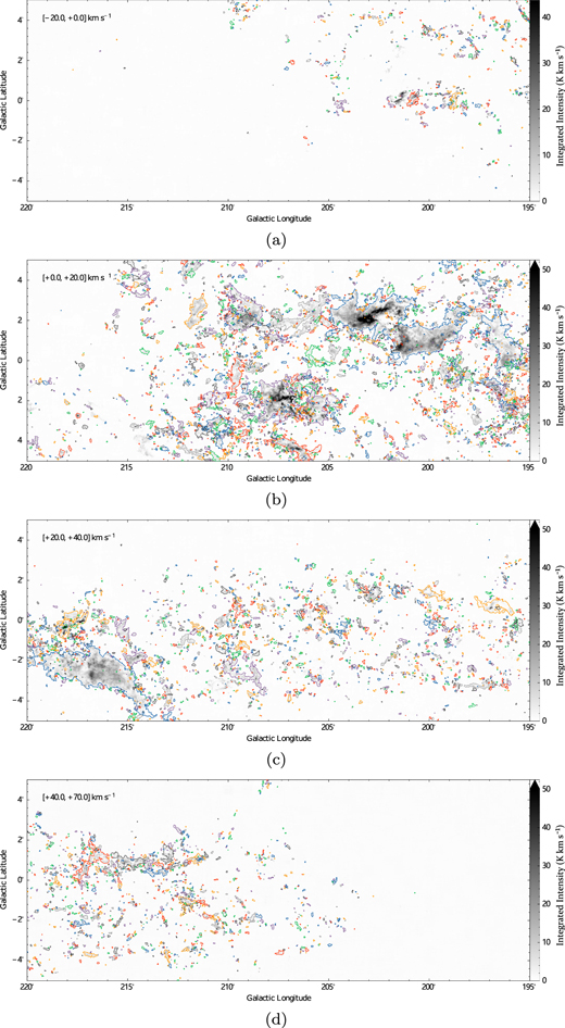
Figure 5. The spatial distribution of all 7069 clouds. The background is the 12CO integrated intensity map within the velocity ranges of [−20, 0], [0, 20], [20, 40], and [40, 70] km s−1, respectively. The boundaries of the MC are outlined with different colored lines and are shown in four velocity intervals depending on the peak velocity of the cloud.
Download figure:
Standard image High-resolution imageTable 1 shows the basic parameters of 12CO for 7069 clouds. The cloud names are listed in Column (1), and the Galactic coordinates and velocity VLSR of peak 12CO intensity are listed in Columns (2)–(4). Columns (5)–(8) present the projected angular area of clouds, velocity dispersion of average spectrum δv , peak intensity, and flux of 12CO line emission flux, respectively. The velocity dispersion of average spectrum and flux can be calculated according to the following formula (Rosolowsky & Leroy 2006):

Table 1. A Catalog of All Molecular Clouds
| Name | lpeak | bpeak | VLSR | Area | δv | Tpeak | Flux |
|---|---|---|---|---|---|---|---|
| (deg) | (deg) | (km s−1) | (arcmin2) | (km s−1) | (K) | (K km s−1 arcmin2) | |
| (1) | (2) | (3) | (4) | (5) | (6) | (7) | (8) |
| G195.000−03.458+005.87 | 195.000 | −03.458 | 5.87 | 142.75 | 0.97 | 6.0 | 262.1 |
| G195.000−03.433+007.94 | 195.000 | −03.433 | 7.94 | 04.25 | 0.30 | 2.8 | 2.7 |
| G195.000−01.575+013.33 | 195.000 | −01.575 | 13.33 | 94.00 | 1.41 | 13.4 | 748.8 |
| G195.000−00.917+017.46 | 195.000 | −00.917 | 17.46 | 07.25 | 0.43 | 2.5 | 5.9 |
| G195.000+01.725+007.94 | 195.000 | +01.725 | 7.94 | 29.75 | 0.64 | 6.9 | 59.4 |
| G195.008+00.125+008.41 | 195.008 | +00.125 | 8.41 | 06.00 | 0.80 | 3.2 | 7.8 |
| G195.008+00.192+003.49 | 195.008 | +00.192 | 3.49 | 09.50 | 0.39 | 2.7 | 7.0 |
| G195.008+00.467+008.10 | 195.008 | +00.467 | 8.10 | 190.00 | 1.14 | 5.6 | 490.8 |
| G195.017−03.033+020.64 | 195.017 | −03.033 | 20.64 | 04.75 | 0.34 | 3.5 | 4.4 |
| G195.017+01.558+007.30 | 195.017 | +01.558 | 7.30 | 26.25 | 0.48 | 4.5 | 25.1 |
| G195.017+03.925−009.68 | 195.017 | +03.925 | −9.68 | 08.25 | 0.39 | 2.7 | 5.4 |
| G195.025−01.083+027.30 | 195.025 | −01.083 | 27.30 | 08.75 | 0.55 | 2.5 | 7.0 |
| G195.025+00.708+005.24 | 195.025 | +00.708 | 5.24 | 02.75 | 0.21 | 2.4 | 1.2 |
| G195.033−02.808+009.68 | 195.033 | −02.808 | 9.68 | 24.00 | 0.59 | 3.4 | 28.2 |
| G195.042−02.700+006.98 | 195.042 | −02.700 | 6.98 | 31.75 | 0.67 | 3.6 | 38.1 |
| G195.042−00.183+023.02 | 195.042 | −00.183 | 23.02 | 12.50 | 0.38 | 3.9 | 13.5 |
| G195.042+00.792+013.33 | 195.042 | +00.792 | 13.33 | 18.75 | 0.63 | 3.5 | 26.3 |
| G195.042+01.600+005.40 | 195.042 | +01.600 | 5.40 | 101.75 | 0.61 | 4.9 | 137.3 |
| G195.058−03.100+023.18 | 195.058 | −03.100 | 23.18 | 02.75 | 0.24 | 2.2 | 1.5 |
| G195.058+02.658+005.87 | 195.058 | +02.658 | 5.87 | 07.25 | 0.37 | 2.8 | 5.1 |
| G195.067−01.025+017.78 | 195.067 | −01.025 | 17.78 | 21.25 | 0.85 | 3.2 | 37.4 |
| G195.067−00.108−005.40 | 195.067 | −00.108 | −5.40 | 29.75 | 0.75 | 4.1 | 46.0 |
| G195.067+04.067−006.98 | 195.067 | +04.067 | −6.98 | 06.25 | 0.27 | 3.0 | 3.9 |
| G195.075−03.667+011.43 | 195.075 | −03.667 | 11.43 | 13.50 | 0.84 | 2.9 | 19.5 |
| G195.075+00.250+002.86 | 195.075 | +00.250 | 2.86 | 06.50 | 0.41 | 2.2 | 6.4 |
| G195.075+03.017+007.62 | 195.075 | +03.017 | 7.62 | 02.50 | 0.26 | 2.2 | 1.5 |
| G195.083−03.017+021.59 | 195.083 | −03.017 | 21.59 | 02.75 | 0.40 | 2.2 | 1.8 |
| G195.092−02.933+002.06 | 195.092 | −02.933 | 2.06 | 07.50 | 0.44 | 3.2 | 6.7 |
| G195.092+04.008−010.79 | 195.092 | +04.008 | −10.79 | 29.00 | 0.36 | 4.0 | 27.6 |
| G195.092+04.933−005.24 | 195.092 | +04.933 | −5.24 | 04.00 | 0.36 | 2.6 | 3.4 |
| G195.100−00.442+003.65 | 195.100 | −00.442 | 3.65 | 661.00 | 1.11 | 7.6 | 3048.0 |
| G195.100+00.133−004.60 | 195.100 | +00.133 | −4.60 | 14.00 | 0.38 | 3.5 | 15.1 |
| G195.100+00.742+004.92 | 195.100 | +00.742 | 4.92 | 07.75 | 0.37 | 3.4 | 6.3 |
| G195.100+00.767+014.92 | 195.100 | +00.767 | 14.92 | 04.75 | 0.36 | 2.1 | 2.3 |
| G195.100+03.858+013.81 | 195.100 | +03.858 | 13.81 | 17.00 | 0.51 | 3.3 | 16.8 |
| G195.100+04.108−010.16 | 195.100 | +04.108 | −10.16 | 92.75 | 0.94 | 4.4 | 123.0 |
| G195.117−01.725+011.75 | 195.117 | −01.725 | 11.75 | 07.75 | 0.39 | 2.6 | 5.4 |
| G195.125−00.067+007.46 | 195.125 | −00.067 | 7.46 | 60.00 | 1.10 | 3.3 | 60.9 |
| G195.133−04.025+005.40 | 195.133 | −04.025 | 5.40 | 02.75 | 0.35 | 2.9 | 1.8 |
| G195.133−03.058+002.70 | 195.133 | −03.058 | 2.70 | 15.00 | 0.63 | 6.8 | 25.5 |
Note. Columns are cloud names, the position and velocity of maximum of 12CO channels in Galactic coordinates, projected angular area of clouds, line width of average spectrum based on second moment, peak intensity, and flux of 12CO, respectively. Only part of the table is shown here owing to space constraints; it is available in its entirety from the online journal. The noise-masked fits files for the 12CO, 13CO, and C18O emission. 1
1 The figure files used in this work are available via the link: https://www.scidb.cn/s/Ubaqqy.Only a portion of this table is shown here to demonstrate its form and content. A machine-readable version of the full table is available.
Download table as: DataTypeset image
Here Ti
is the main-beam brightness temperature of 12CO, and  is mean velocity. The sums run over all emission in the cloud. The definitions of velocity dispersion and flux also apply to 13CO and C18O.
3.2. 13CO Emission
Even though thousands of MCs are identified by DBSCAN, the portion of clouds that contain 13CO and C18O emission is unknown. Stacking multiple spectra is often used in the study of extragalactic galaxies, and it is good at finding weak signals. In this study, we develop two algorithms for identifying 13CO and C18O signals based on spectral stacking, named stacking bump and stacking intensity, respectively. We also tried to use the DBSCAN algorithm to search for 13CO and C18O signals. Through the comparison of these three algorithms (Section 5), we find that the stacking bump at 2σ algorithm is more suitable for searching for 13CO and C18O signals in our datacube. This section mainly introduces the stacking bump at 2σ algorithm, and the results of the other two algorithms are shown in Section 5.
Since 13CO and C18O are less abundant than 12CO, the intensities of 13CO and C18O are significantly lower than 12CO emission. The weak parts of 13CO and C18O emissions are more likely present in the spectrum as bump features owing to spectral noise. The basic principle of the stacking bump algorithm is to search for the bump in the original spectrum of 13CO and C18O according to a specific signal-to-noise ratio (S/N) within the 12CO boundary in PPV space, then average the spectrum containing bump components, and finally identify the emission of 13CO and C18O based on the S/N of the average spectrum.
The basic steps of the stacking bump at 2σ algorithm mainly include four steps. The first step is to determine the cloud boundary in PPV space. In this paper, we determine the cloud boundary based on the DBSCAN algorithm from the 12CO datacube as shown in Section 3.1. The second step is to search for the bump in the original spectrum of 13CO and C18O within the 12CO boundary in PPV space. The bump is defined based on the criterion that three contiguous channels were larger than a certain value threshold (such as 1.5σ or 2σ; different thresholds result in different signal number and flux; see Section 5). The third step is to average this bump-feature spectrum and calculate the noise of the average spectrum σa
(σa
=  , where Nspectrum is the spectrum number involved in averaging). The average spectrum for 13CO and C18O will be identified as a signal based on the criterion that it should contain at least three consecutive channels with intensities above 3σ
a
. The last step is to check the spectrum and remove the false detection caused by the wavelike baseline through visual inspection by comparing the average spectral lines of 13CO and C18O of these identified signals with the spectra of 12CO. All the steps are based on the S/N values to identify the signals, except in the last step, which is to manually check for wavelike baseline interference.
, where Nspectrum is the spectrum number involved in averaging). The average spectrum for 13CO and C18O will be identified as a signal based on the criterion that it should contain at least three consecutive channels with intensities above 3σ
a
. The last step is to check the spectrum and remove the false detection caused by the wavelike baseline through visual inspection by comparing the average spectral lines of 13CO and C18O of these identified signals with the spectra of 12CO. All the steps are based on the S/N values to identify the signals, except in the last step, which is to manually check for wavelike baseline interference.
Based on the above principles and basic steps, we summarize four criteria for the identification of the 13CO signal. (1) Three contiguous channels in the 13CO spectrum were larger than 2σ (∼0.38 K). (2) At least one of its eight adjacent pixels satisfies condition 1. (3) Each cloud must have at least two pixels. (4) The average spectrum based on these pixels has three consecutive channels above 3σa . Based on these criteria and manual examination of the 12CO and 13CO average spectrum, a total of 1197 clouds with 13CO signals have been identified.
The basic parameters of 13CO for 1197 clouds are listed in Table 2, including names, the position and velocity of maximum of 13CO, projected angular area, velocity dispersion of average spectrum, peak intensity, and 13CO flux. These parameters are defined in the same way as in Table 1.
Table 2. A Catalog of Molecular Clouds Identified with 13CO Emission
| Name |

|

|

| Area13 |

|

| Flux13 |
|---|---|---|---|---|---|---|---|
| (deg) | (deg) | (km s−1) | (arcmin2) | (km s−1) | (K) | (K km s−1 arcmin2) | |
| (1) | (2) | (3) | (4) | (5) | (6) | (7) | (8) |
| G195.000−03.458+005.87 | 195.000 | −03.475 | +5.65 | 1.75 | 0.47 | 1.3 | 1.3 |
| G195.000−01.575+013.33 | 195.000 | −01.567 | +13.45 | 44.25 | 1.17 | 4.3 | 123.8 |
| G195.000+01.725+007.94 | 195.000 | +01.725 | +7.80 | 6.75 | 0.42 | 2.7 | 7.5 |
| G195.067−01.025+017.78 | 195.058 | −01.025 | +18.43 | 5.25 | 0.69 | 1.6 | 5.6 |
| G195.100−00.442+003.65 | 195.100 | −00.450 | +3.65 | 68.50 | 0.77 | 2.1 | 68.1 |
| G195.100+04.108−010.16 | 195.108 | +04.117 | −10.29 | 0.75 | 0.28 | 1.0 | 0.4 |
| G195.133−03.058+002.70 | 195.133 | −03.058 | +2.99 | 1.25 | 0.35 | 1.0 | 0.8 |
| G195.133+01.792+004.44 | 195.133 | +01.792 | +4.32 | 0.50 | 0.24 | 0.7 | 0.2 |
| G195.175+00.400−006.83 | 195.183 | +00.358 | −6.64 | 3.75 | 0.45 | 1.3 | 2.7 |
| G195.233−03.300+003.81 | 195.267 | −03.317 | +3.65 | 1.25 | 0.50 | 1.0 | 1.0 |
| G195.367−02.875+011.91 | 195.283 | −02.775 | +10.96 | 3.50 | 0.57 | 1.1 | 2.5 |
| G195.292−02.242+018.73 | 195.292 | −02.250 | +18.93 | 3.50 | 0.44 | 1.8 | 3.9 |
| G195.008+00.467+008.10 | 195.325 | +00.583 | +4.82 | 7.50 | 1.39 | 1.2 | 5.8 |
| G195.350+04.350−013.65 | 195.342 | +04.350 | −13.62 | 1.25 | 0.59 | 1.3 | 0.6 |
| G195.358+01.325+006.83 | 195.358 | +01.333 | +6.48 | 1.00 | 0.38 | 1.1 | 0.8 |
| G195.408−02.708+012.06 | 195.417 | −02.700 | +12.45 | 1.00 | 0.83 | 0.9 | 1.1 |
| G195.442+01.050+009.84 | 195.433 | +01.050 | +9.96 | 7.50 | 0.42 | 2.5 | 7.8 |
| G195.400+04.258+010.79 | 195.442 | +04.267 | +11.46 | 0.75 | 0.30 | 0.8 | 0.4 |
| G195.458−00.133+020.64 | 195.475 | +00.000 | +19.76 | 176.50 | 0.67 | 3.6 | 286.6 |
| G195.475−00.500+020.79 | 195.508 | −00.508 | +19.92 | 25.50 | 0.65 | 2.9 | 41.3 |
| G195.542−01.992+015.56 | 195.533 | −02.000 | +15.44 | 134.50 | 1.01 | 3.3 | 202.8 |
| G195.550+00.467+031.91 | 195.533 | +00.483 | +32.38 | 25.00 | 0.75 | 3.4 | 42.4 |
| G195.575−00.200+015.72 | 195.542 | −00.092 | +14.45 | 5.00 | 0.60 | 1.8 | 4.0 |
| G195.625+00.525+032.07 | 195.642 | +00.517 | +31.71 | 2.75 | 0.44 | 1.3 | 2.2 |
| G195.650−00.067+032.07 | 195.650 | −00.067 | +32.21 | 116.75 | 1.51 | 5.8 | 332.6 |
| G195.658+00.350−006.67 | 195.650 | +00.358 | −6.14 | 1.50 | 0.37 | 1.2 | 0.8 |
| G195.667−02.633+011.75 | 195.658 | −02.650 | +11.46 | 11.50 | 0.52 | 1.6 | 10.1 |
| G195.667−04.150+024.92 | 195.667 | −04.142 | +24.91 | 0.75 | 0.30 | 0.9 | 0.3 |
| G195.692−00.567+033.18 | 195.683 | −00.567 | +33.04 | 2.50 | 0.33 | 1.6 | 1.9 |
| G195.692−02.800+013.97 | 195.692 | −02.800 | +13.78 | 0.50 | 0.43 | 0.8 | 0.3 |
| G195.717−02.708+010.00 | 195.717 | −02.708 | +9.80 | 4.25 | 0.91 | 1.2 | 3.6 |
| G195.717−01.383+013.02 | 195.717 | −01.383 | +13.12 | 1.75 | 0.75 | 1.1 | 1.7 |
| G195.675−02.342+004.60 | 195.742 | −02.300 | +4.32 | 203.50 | 0.59 | 7.7 | 508.1 |
| G195.767+01.917-009.37 | 195.758 | +01.892 | −8.63 | 0.50 | 0.39 | 0.7 | 0.4 |
| G195.775−01.933+018.25 | 195.775 | −01.933 | +18.60 | 1.00 | 0.28 | 1.0 | 0.7 |
| G195.783−02.050+014.29 | 195.783 | −02.058 | +15.28 | 0.50 | 0.55 | 0.8 | 0.4 |
| G195.800−03.575+013.33 | 195.800 | −03.592 | +13.62 | 9.75 | 0.47 | 1.7 | 9.0 |
| G196.050−02.583+006.83 | 195.808 | −02.400 | +10.13 | 11.75 | 1.23 | 1.5 | 7.8 |
| G195.833−00.358+035.72 | 195.833 | −00.358 | +35.86 | 0.75 | 0.47 | 1.1 | 0.6 |
| G195.883−00.692+017.30 | 195.883 | −00.683 | +17.43 | 3.00 | 0.81 | 1.5 | 3.0 |
Note. Columns are cloud names, the position and velocity of maximum of 13CO channels in Galactic coordinates, projected angular area of clouds, line width of average spectrum, peak intensity, and flux of 13CO. The entire table (1197 clouds) is available from the online journal.
Only a portion of this table is shown here to demonstrate its form and content. A machine-readable version of the full table is available.
Download table as: DataTypeset image
3.3. C18O Emission
The emission of C18O is significantly weaker than 12CO and 13CO, so the extraction of the C18O signal should be very cautious. As discussed in Section 5, the stacking bump at 2σ algorithm is suitable not only for searching for 13CO signals but also for searching for C18O signals. In this section, we only introduce and show the results of the stacking bump at 2σ algorithm in searching for C18O signals, and the comparison with other algorithms will be mainly shown in Section 5.
The basic principle and steps of the stacking bump at 2σ algorithm are shown in Section 3.2. The steps and criteria of searching for 13CO and C18O signals are basically the same.
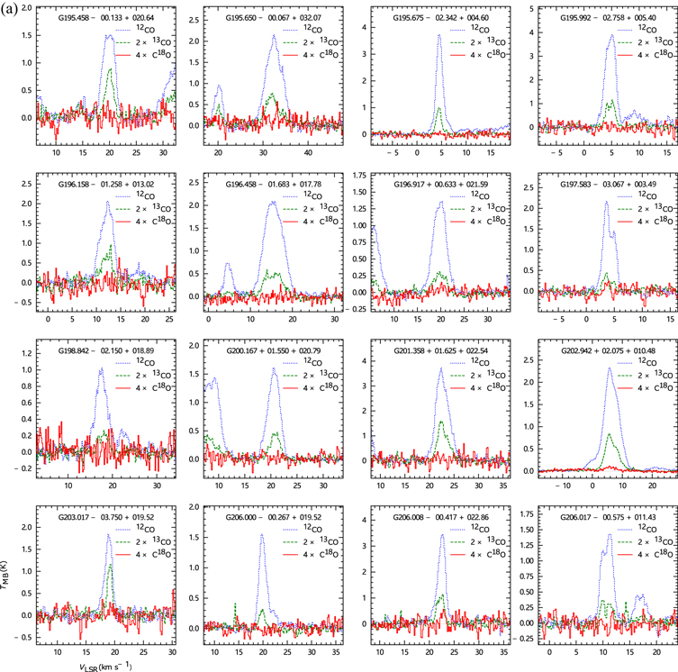
According to the above discussion on the difference between searching for 13CO and C18O signals, we summarize the following four criteria for searching for C18O signals: (1) Three contiguous channels in the C18O spectrum were larger than 2σ (∼0.5 K). (2) At least one of its eight adjacent pixels identically satisfies condition 1. (3) Each cloud must have at least two pixels. (4) The average spectrum based on these pixels has three consecutive channels above the 3σa threshold. These four conditions are basically the same as those for selecting 13CO signals. Finally, by checking the average spectra of the three molecular lines 12CO, 13CO, and C18O, 32 MCs were confirmed to contain C18O emission.
Figures 6(a)–(b) show the average spectra of 12CO, 13CO, and C18O for 32 clouds detected in C18O. Different algorithms can lead to differences in the measurement of C18O flux, and we will discuss this effect in detail in Section 5.
Download figure:
Standard image High-resolution image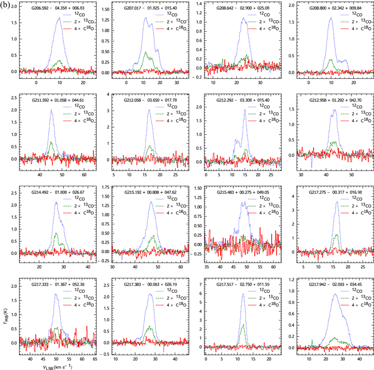
Figure 6. (a) The average spectrum of 32 clouds considered containing C18O emission. Different colors and line types represent different CO isotopologues. The spectra of different isotopologues are averaged for all pixels in the cloud. (b) Continuation of panel (a).
Download figure:
Standard image High-resolution imageTable 3 lists the basic parameters of C18O emission for 32 clouds. The columns are the same as in Tables 1 and 2, but they are calculated from C18O data.
Table 3. A Catalog of Molecular Clouds Identified with C18O Emission
| Name |

|

|

| Area18 |

|

| Flux18 |
|---|---|---|---|---|---|---|---|
| (deg) | (deg) | (km s−1) | (arcmin2) | (km s−1) | (K) | (K km s−1 arcmin2) | |
| (1) | (2) | (3) | (4) | (5) | (6) | (7) | (8) |
| G195.458−00.133+020.64 | 195.450 | −00.125 | +18.86 | 1.25 | 0.78 | 1.2 | 1.4 |
| G195.675−02.342+004.60 | 195.717 | −02.308 | +4.36 | 14.25 | 0.85 | 1.9 | 17.6 |
| G195.650−00.067+032.07 | 195.817 | −00.208 | +30.03 | 1.75 | 1.53 | 1.5 | 2.8 |
| G195.992−02.758+005.40 | 195.992 | −02.733 | +3.86 | 0.75 | 0.87 | 0.9 | 0.4 |
| G196.158−01.258+013.02 | 196.158 | −01.250 | +12.19 | 0.50 | 1.82 | 0.9 | 0.7 |
| G196.458−01.683+017.78 | 196.408 | −01.708 | +17.03 | 4.75 | 1.46 | 1.2 | 6.4 |
| G196.917+00.633+021.59 | 196.967 | +00.583 | +19.36 | 1.75 | 1.37 | 1.1 | 1.6 |
| G197.583−03.067+003.49 | 197.658 | −03.083 | +3.19 | 1.50 | 0.29 | 1.5 | 1.0 |
| G198.842−02.150+018.89 | 198.850 | −02.158 | +18.03 | 2.25 | 1.73 | 1.2 | 2.5 |
| G200.167+01.550+020.79 | 199.900 | +01.225 | +21.03 | 3.75 | 0.75 | 1.3 | 4.0 |
| G201.358+01.625+022.54 | 201.375 | +01.600 | +22.53 | 1.00 | 1.27 | 0.9 | 1.1 |
| G203.017−03.750+019.52 | 203.017 | −03.733 | +19.19 | 1.25 | 0.26 | 1.2 | 0.5 |
| G202.942+02.075+010.48 | 203.217 | +02.075 | +5.03 | 1028.00 | 2.12 | 3.5 | 1363.0 |
| G206.000−00.267+019.52 | 205.892 | +00.167 | +20.03 | 0.50 | 0.27 | 1.1 | 0.2 |
| G206.008−00.417+022.86 | 206.025 | −00.417 | +21.86 | 2.00 | 1.28 | 1.5 | 3.2 |
| G206.017−00.575+011.43 | 206.267 | −00.700 | +10.03 | 1.00 | 0.63 | 1.0 | 0.3 |
| G206.592−04.358+006.83 | 206.875 | −04.375 | +9.19 | 1.50 | 1.31 | 1.1 | 1.5 |
| G207.017−01.825+015.40 | 207.108 | −01.833 | +10.69 | 362.50 | 2.61 | 2.6 | 462.5 |
| G208.800+02.342+009.84 | 208.533 | +02.375 | +9.03 | 17.75 | 0.64 | 1.2 | 8.4 |
| G208.642−02.900+025.08 | 208.625 | −02.892 | +25.03 | 5.75 | 1.37 | 1.6 | 7.2 |
| G211.592+01.058+044.61 | 211.517 | +00.975 | +44.36 | 2.75 | 1.57 | 1.2 | 2.2 |
| G212.058−03.650+017.78 | 212.058 | −03.633 | +17.69 | 2.25 | 0.59 | 1.5 | 2.0 |
| G212.292−03.308+015.40 | 212.317 | −03.333 | +16.03 | 1.75 | 0.91 | 1.0 | 1.5 |
| G212.958+01.292+042.70 | 212.950 | +01.300 | +42.53 | 3.25 | 1.35 | 1.1 | 3.1 |
| G215.192+00.808+047.62 | 214.700 | +00.708 | +47.53 | 6.25 | 1.37 | 1.2 | 6.0 |
| G214.492−01.808+026.67 | 215.075 | −01.758 | +27.03 | 11.25 | 1.70 | 1.4 | 9.7 |
| G215.483+00.275+049.05 | 215.492 | +00.250 | +48.69 | 0.50 | 0.81 | 0.9 | 0.3 |
| G217.942−02.083+034.45 | 216.775 | −02.650 | +23.69 | 18.25 | 2.33 | 1.3 | 13.8 |
| G217.275−00.317+016.98 | 217.242 | −00.242 | +16.03 | 3.75 | 0.59 | 1.5 | 3.7 |
| G217.333−01.367+052.38 | 217.333 | −01.367 | +50.36 | 0.50 | 1.45 | 1.2 | 0.8 |
| G217.517−02.750+011.59 | 217.500 | −02.758 | +10.86 | 1.00 | 0.64 | 1.0 | 0.9 |
| G217.383−00.083+026.19 | 218.175 | −00.675 | +25.19 | 60.00 | 1.45 | 2.1 | 81.2 |
Note. Columns are cloud names, the position and velocity of maximum of C18O channels in Galactic coordinates, projected angular area of clouds, line width of average spectrum, peak intensity, and flux of C18O. The entire table (32 clouds) is available from the online journal.
Only a portion of this table is shown here to demonstrate its form and content. A machine-readable version of the full table is available.
Download table as: DataTypeset image
4. Statistics
4.1. Detection Rate
A total of 7069 clouds were identified based on the DBSCAN algorithm in the 12CO data. We identified 1197 clouds having 13CO emission and 32 clouds having C18O emission based on the stacking bump algorithm in the catalog of 7069 clouds, respectively. The detection rate of C18O, defined by the number of C18O-emitting clouds divided by the number of 12CO clouds, is 0.5%, much lower than the detection rate of 13CO (16.9%).
Figure 7 presents 13CO and C18O percentage rates of clouds against different parameters (peak intensity, projected area, and total flux). The rate is the percentage of clouds with 13CO (red triangles) and C18O (blue circles) emission. The percentage rate of 13CO increases rapidly with all three parameters and stays at 100% above a certain parameter region ( > 10 K, 12CO projected area >500 arcmin2, 12CO flux >1000 K km s−1 arcmin2). The percentage rate of C18O increases slowly with increasing parameters and reaches 100% after dropping or flattening.
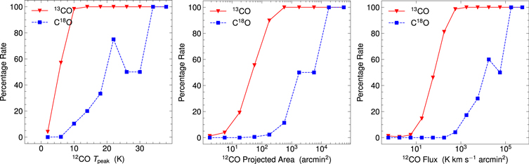
Figure 7. 13CO and C18O percentage rates of clouds with different parameters (peak intensity, projected area, and total flux).
Download figure:
Standard image High-resolution imageFigure 8 shows 13CO and C18O percentage rates pixel by pixel against different spectral parameters (peak intensity, integrated intensity). The percentage rate of 13CO increases rapidly with 12CO peak and intensity, with a peak of 9 K or intensity of 30 K km s−1 giving a 100% percentage rate. The percentage rate of C18O increases slowly with increasing 12CO peak and intensity. Above the integrated intensity of 140 K km s−1 of the 12CO emission, the percentage rate of C18O reaches 100%.
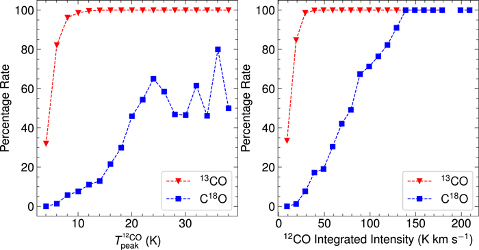
Figure 8. 13CO and C18O percentage rates pixel by pixel against different spectral parameters (peak intensity, integrated intensity).
Download figure:
Standard image High-resolution imageSurprisingly, the percentage rate of C18O drops and stays between 50% and 80% when the 12CO peak value is greater than 24 K. Notably, the pixels with 12CO Tpeak greater than 24 K come from six MCs (G202.942+02.075+010.48, G207.017−01.825+015.40, G196.458−01.683+017.78, G217.383−00.083+026.19, G196.825−03.108+025.56, and G211.250−00.375+021.27). In four of the six clouds, C18O emission was detected (G202.942+02.075+010.48, G207.017−01.825+015.40, G196.458−01.683+017.78, and G217.383−00.083+026.19), while the pixels with  greater than 24 K but without C18O detection come from three clouds (G202.942+02.075+010.48, known as NGC 2264; G207.017−01.825+015.40, known as the Rosette Nebula; and G196.458−01.683+017.78). Among these three clouds, the pixels with
  greater than 24 K but without C18O detection are only distributed at the boundary of the dense regions and in an arc shape. There are strong radiation fields around these regions, suggesting that the depletion of C18O could come from the selective photodissociation of C18O by the radiation field. 12CO and 13CO are preserved owing to the self-shielding effect.
4.2. Statistical Results
The peak velocity distributions of clouds that have 12CO, 13CO, and C18O emissions are shown in Figure 9. The Vpeak distribution of clouds with 12CO emission has four components that peak at −10, 10, 23, and 42 km s−1. The Vpeak distribution of 13CO follows that of 12CO and also has four components. However, for C18O, the first component in the Vpeak distribution of −10 km s−1 is absent.
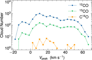
Figure 9. The peak velocity distribution of the clouds. The y-axis is the cloud number to find a peak velocity of a cloud within 4 km s−1 around the bin center, which is marked with circles, inverted triangles, and squares for the 12CO, 13CO, and C18O emission, respectively.
Download figure:
Standard image High-resolution imageFigure 10 shows the basic properties of the cloud, including peak intensity, projected angular area, line width of average spectrum, and flux. The 12CO peak intensity  ranges from 1.4 to 37.5 K and follows a power-law distribution. We fit the power-law distributions of peak intensity, projected area, line width, and flux by the formula

where X is the derived parameter. The fitting index α of  is 4.23. Although the maximum
  and
and  are only 15 and 3.5 K, respectively, which are lower than
  , they have indices similar to
  , which are 3.61 and 3.58, respectively. It should be noted that the range and sample number of
  are not sufficient to obtain the fitting error. In comparison with the index of
  in the second quadrant (Yuan et al. 2021), which is 2.8, we find that the α here is quite different.
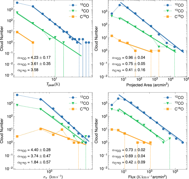
Figure 10. Distributions of the basic properties of the cloud, including peak intensity, projected angular area, velocity dispersion of average spectrum, and flux. The colors represent different isotopologues. Each point is the value of the probability density function at the bin, normalized such that the integral over the range is 1. Without bins with unity width, the histogram values will not sum up to 1. The solid lines fit the power-law distributions of basic properties, with the formula dN/dX ∝ X−(α+1). The results of index α are shown in the figures with errors, but the error of  cannot be calculated because of poor pixel number and distribution region.
Download figure:
Standard image High-resolution imageThe statistical results of 12CO projected angular area are distributed in [1, 3.6 × 10⁴] arcmin2, which spans four orders of magnitude. The distribution range of 13CO is slightly narrower than 12CO with a maximum of 1.3 × 10⁴, while the range of C18O is much narrow than 12CO with a maximum of 1.5 × 10³. The fitting indices α of the distribution of the 12CO, 12CO, and C18O clouds are 0.96, 0.75, and 0.41, respectively. In comparison with index of 12CO projected angular area in the second quadrant (Yuan et al. 2021), which is 1.9, our projected angular area is flatter.
Velocity dispersion δv of the average spectrum traced by different isotopologues is shown in Figure 10. The ranges of 12CO, 13CO, and C18O are [0.1, 4.3], [0.2, 5.2], and [0.5, 4.6] km s−1, respectively. The fitting indices of δv are 4.4, 3.7, and 1.8 for 12CO, 13CO, and C18O, respectively. Ma et al. (2022) found a relation between the dispersion of normalized column density and the sonic Mach number of MCs based on the same data and catalog.
The fluxes of 12CO and 13CO are distributed in the ranges of [0.7, 4.6 × 10⁵] and [0.2, 6.8 × 10⁴] K km s−1 arcmin2, respectively. While the C18O flux only distributed in the range of [1.7 × 10⁻³, 1.7 × 10³], its maximum flux is lower than 12CO and 13CO by two and one orders of magnitude, respectively. The flux power-law indices are 0.73, 0.69, and 0.42 for 12CO, 13CO, and C18O, respectively. Details will be discussed in our next paper (Wang et al., in preparation).
5. Discussion
5.1. Algorithms
Large-scale sample studies of MCs help us to understand the basic properties of MCs. But the creation of MC samples depends on algorithms. Clipping (Dame 2011), DBSCAN (Yan et al. 2020), and moment mask (Dame 2011) algorithms are commonly used. Yuan et al. (2022) used these three different methods to extract the 13CO gas structures within each 12CO cloud based on the counterpart data of the MWISP project in the second Galactic quadrant. They concluded that the clipping extracts plenty of noise spikes with values larger than the 4σ threshold while losing a significant part of faint emission having intensities less than 4σ. The moment mask leaves out a part of faint and tiny 13CO structures, due to the smooth procedure. The DBSCAN algorithm can not only avoid the noise spikes but also preserve the faint and tiny 13CO structures not identified by the moment mask. This indicates that the DBSCAN algorithm is better than the other two algorithms for searching for 13CO and C18O signals in our data. Therefore, in this paper we mainly compare the differences between DBSCAN and the new algorithms.
The cloud catalog of this paper is established from the 12CO datacube by the DBSCAN algorithm, which is more appropriate for identifying consecutive structures within the observed PPV space (Yan et al. 2020). Since 13CO and C18O are less abundant than 12CO, one can reasonably assume that the emission of these isotopic lines is within the extent defined by the 12CO boundary in PPV space. Therefore, we made measurements of 13CO and C18O emission within the envelope of each 12CO map. However, since 13CO and C18O are significantly weaker than 12CO, using the same parameters to search for their signals with the DBSCAN algorithm may be questionable because of the low‐S/N of the 13CO and C18O emission. Therefore, the choice of 13CO and C18O signal detection algorithms requires careful comparison. In this study we tried to search for 13CO and C18O signals with three different algorithms, DBSCAN, stacking intensity, and stacking bump.
The first is to directly apply the DBSCAN algorithm to 13CO and C18O. The criteria are shown in Section 3.1. A total of 709 identified clouds have 13CO signals, and 11 clouds have C18O signals.
The alternative algorithm is spectral stacking, which means that the spectra from the same cloud are aggregated to increase the intensity of the signal to meet the detection standard. Stacking multiple spectra based on different criteria may reduce the noise. However, an arbitrary increase of the number of spectra may also reduce the signal's strength. The result is sensitive to the selection of channel (velocity) range. We chose two methods to identify the possible signal range. One is based on the 3σ of the velocity-integrated intensity pixel (pixel is the position in the spatial map; we named it the stacking intensity algorithm), and the other is by looking for weak bumps in the original spectrum that might be weak signals (we named it stacking bump, as we presented in Sections 3.2 and 3.3).
The principle of the stacking intensity algorithm is to search for pixels identified as possible signals based on the S/N threshold in the intensity map of 13CO and C18O. Then, we average the spectrum of those pixels. Finally, we identify the emission of 13CO and C18O based on the S/N of the average spectrum. The principle of the stacking intensity algorithm is similar to the principle of the stacking bump algorithm, but there are differences in how to select the spectrum.
The basic steps of the stacking intensity algorithm mainly include four steps similar to the stacking bump algorithm. The first step is to determine the cloud boundary in PPV space as we do in Section 3.1. 13CO and C18O intensity is integrated within channel (velocity) range based on the envelope obtained by the DBSCAN algorithm in the 12CO datacube. The second step is to select pixels in the intensity map of 13CO and C18O. The selected criterion is that 13CO and C18O intensity is above the triple intensity noise threshold (σi
=  , where Nchannels is the channel number in the spectrum). The third step is to average those pixels' spectra and calculate the noise of the average spectrum σa
. The average spectrum will be identified as a signal based on the criterion of three consecutive channels above the 3σa
threshold for 13CO, but the 2σa
threshold for C18O. The last step is to check the spectrum and remove the false detection caused by the wavelike baseline through visual inspection by comparing the average spectral lines of 13CO and C18O of these identified signals with the spectra of 12CO. The last two steps of the stacking intensity algorithm are consistent with the stacking bump, and the signal is identified by the S/N values in the step, instead of being identified artificially.
, where Nchannels is the channel number in the spectrum). The third step is to average those pixels' spectra and calculate the noise of the average spectrum σa
. The average spectrum will be identified as a signal based on the criterion of three consecutive channels above the 3σa
threshold for 13CO, but the 2σa
threshold for C18O. The last step is to check the spectrum and remove the false detection caused by the wavelike baseline through visual inspection by comparing the average spectral lines of 13CO and C18O of these identified signals with the spectra of 12CO. The last two steps of the stacking intensity algorithm are consistent with the stacking bump, and the signal is identified by the S/N values in the step, instead of being identified artificially.
According to the principles and basic steps of stacking intensity, we summarize four criteria for the identification of 13CO and C18O signals. (1) According to the envelope of MCs obtained by the DBSCAN algorithm in the 12CO datacube, 13CO and C18O intensity is integrated along velocity. 13CO and C18O integrated intensity is above the 3σi threshold. (2) At least one of its eight adjacent pixels satisfies condition 1. (3) Each cloud must have at least two pixels. (4) The average spectrum based on these pixels has three consecutive channels above the 3σa threshold for 13CO and C18O. Based on these criteria and manual examination of the average spectrum, a total of 1128 clouds had 13CO signals and 32 clouds had C18O signals (Table 4).
Table 4. 13CO and C18O Signal Number and Detectivity
| Algorithms | 13CO | C18O | ||
|---|---|---|---|---|
| Number | Detection Rate | Number | Detection Rate | |
| (1) | (2) | (3) | (4) | (5) |
| DBSCAN | 708 | 10% | 11 | 0.16% |
| Stacking intensity | 1107 | 16% | 34 | 0.48% |
| Stacking bump at 1.5σ | 1389 | 20% | 56 | 0.79% |
| Stacking bump at 2σ | 1197 | 17% | 32 | 0.5% |
Download table as: ASCIITypeset image
Another spectral stacking algorithm is stacking bump. It is to search the bump in the original spectrum of 13CO and C18O based on the criterion that three contiguous channels were larger than a certain value threshold (1.5σ or 2σ). These bumps are most likely to be weak signals of 13CO and C18O. Finally, the signal was identified by stacking these spectra containing the bump according to the S/N values. Since the stacking bump algorithm is sensitive to the criterion of the 1.5σ or 2σ threshold in spectrum, we test these two thresholds when using it to search for the bump. The first threshold is 2σ, shown in Sections 3.2 and 3.3, and named as stacking bump at 2σ. The second threshold is 1.5σ, named as stacking bump at 1.5σ. The only difference between these two algorithms is the threshold for the bump, and all steps and criteria of the stacking bump at 2σ algorithm are the same as the stacking bump at 1.5σ algorithm. Based on the stacking bump at 1.5σ algorithm, a total of 1197 clouds had 13CO signals and 33 clouds had C18O signals (Table 4).
In terms of quantity, the number of 13CO and C18O signals found by the DBSCAN algorithm is the least, while the other two algorithms are relatively close to each other. The DBSCAN is good at identifying consecutive structures in PPV space, which is highly dependent on the 2σ threshold. As a result, it may lose some clouds of weak signal.
5.2. Noise Test
The stacking algorithm searches for 13CO or C18O spectra with either "bumps" feature or the 3σ threshold of integrated intensity in a small range of velocity defined by the 12CO emission and then averaging those spectra, which may result in false detection caused by spurious noise spikes. Determining the authenticity of the 13CO or C18O emission requires a noise test for algorithms. We chose two kinds of noise to test the stacking algorithm with different parameters; one is Gaussian noise, and the other is real noise in the velocity range of the spectrum without 12CO emission in the data.
We replace the 13CO and C18O cube with a cube containing only Gaussian noise at the same level as the actual cube, and then we run the stacking algorithm with different parameters on the noise-only cube. Tables 5 and 6 show results of different stacking algorithms according to the 7069-cloud boundary on the noise-only cube. The test results show that, for Gaussian noise, the algorithm can only produce one false detection. However, the real noise of the data may not be Gaussian. It is also necessary to test in real data noise space.
Table 5. A Catalog of Stacking Bump Algorithm Test in Gaussian Noise and Data Noise
| Noise Type | Tracer | rms Threshold | Results |
|---|---|---|---|
| (σ) | (Clouds) | ||
| (1) | (2) | (3) | (4) |
| Gaussian noise | 1 | 0 | |
| 13CO | 1.5 | 1 | |
| 2 | 0 | ||
| 1 | 0 | ||
| C18O | 1.5 | 0 | |
| 2 | 0 | ||
| Data noise in [105, 195] km s−1 | 1 | 75 | |
| 13CO | 1.5 | 28 | |
| 2 | 3 | ||
| 1 | 11 | ||
| C18O | 1.5 | 6 | |
| 2 | 1 | ||
| Data noise in [−135, − 45] km s−1 | 1 | 49 | |
| 13CO | 1.5 | 18 | |
| 2 | 3 | ||
| 1 | 8 | ||
| C18O | 1.5 | 2 | |
| 2 | 3 | ||
Download table as: ASCIITypeset image
Table 6. A Catalog of Stacking Intensity Algorithm Test in Gaussian Noise and Data Noise
| Noise Type | Tracer | rms Threshold | Results |
|---|---|---|---|
| (σ) | (Clouds) | ||
| (1) | (2) | (3) | (4) |
| Gaussian Noise | 13CO | 3 | 0 |
| C18O | 3 | 0 | |
| Data noise in [105, 195] km s−1 | 13CO | 3 | 34 |
| C18O | 3 | 0 | |
| Data noise in [−135, − 45] km s−1 | 13CO | 3 | 17 |
| C18O | 3 | 1 | |
Download table as: ASCIITypeset image
Our observation data are 3D PPV data, and the boundary of these 7069 clouds is a three-dimensional structure distributed in the velocity range [−20, 70] km s−1. In order to test the real data noise on the algorithm, we shifted the boundary of the cloud to the [−135, −45] and [105, 195] km s−1 velocity intervals without signal emission in the velocity dimension space. According to the results of the Columbia CO survey (Dame et al. 2001), there is no CO emission in these two velocity intervals. We also searched for 12CO signals in these two intervals and confirmed that there is no 12CO signal in these two intervals. In addition, we checked data of the Leiden/Argentine/Bonn (LAB) Survey of Galactic H i (Kalberla et al. 2005), and there was also no H i signal in the two velocity intervals. The absence of CO emission indicates that these two intervals are suitable for verifying the algorithm.
We tested the results of the algorithm with different parameters in these two velocity intervals. We tested different rms thresholds in the stacking bump algorithm and the stacking intensity algorithm. The results (Tables 5 and 6) indicate that an rms threshold of 2σ can effectively avoid the possibility of false detections generated by noise. The number of false detections (1–3) generated by the 2σ threshold is very small, far less than the number of 13CO and C18O (1197 and 32) signals identified in [−20, 70] km s−1, and it will not have a significant impact on the results. On the other hand, the stacking intensity algorithm produced more false detection than the stacking bump at 2σ algorithm. Therefore, from these noise tests, it can be determined that the possibility of false detection generated by the stacking bump at 2σ algorithm is very low. It should be noted that the pure noise cube yields so few spurious clouds compared with the number derived from the velocity edges of the real data with the same noise level. Based on the noise statistical distribution (Figure 1), the real noise distribution has Gaussian-like characteristics, but it is not perfect Gaussian noise. This difference between real noise and pure noise cube can lead to more spurious noise spikes in real data. Moreover, a slight difference in the spatial distribution of noise (Figure 2) may also affect the results of signal searching.
5.3. Spatial Distribution of 13CO and C18O Emission
Figure 11 illustrates the spatial boundary of 13CO emission of cloud G207.017−01.825+015.40 (known as the Rosette Nebula; Li et al. 2018) based on different algorithms. The DBSCAN algorithm shows a smooth and coherent structure in the boundary of 13CO compared to other algorithms owing to its high threshold in pixel number, but it does not detect the 13CO emission in some regions with weak 12CO intensity. The other algorithms exhibit similar properties of fragmented spatial distribution in 13CO.
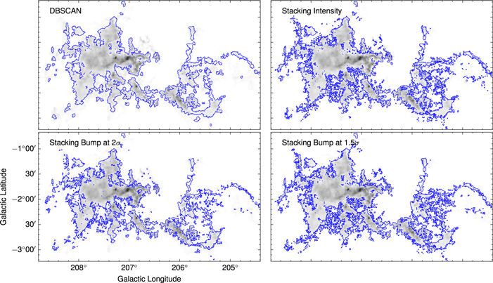
Figure 11. The spatial distribution of 13CO emission in cloud G207.017−01.825+015.40 (known as the Rosette Nebula; Li et al. 2018) based on different algorithms. The background is the 12CO intensity, and the contour shows the boundary of 13CO emission.
Download figure:
Standard image High-resolution imageSimilar maps that show the spatial boundaries of the detected C18O emission within the Rosette Nebula are given in Figure 12. Compared with other algorithms, the results of the stacking bump at 2σ algorithm are more extended than the results of the DBSCAN algorithm and can also detect sporadic distribution in the region with weak 12CO intensity. Although the stacking bump at 1.5σ algorithm can detect the widest area of C18O emission, it may lead to false high-σ signals owing to its low 1.5σ threshold, as confirmed in Section 5.2.
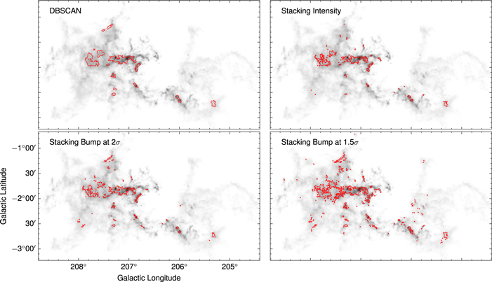
Figure 12. The spatial distribution of C18O emission in cloud G207.017−01.825+015.40 (known as the Rosette Nebula; Li et al. 2018) based on different algorithms. The background is the 12CO intensity, and the contour shows the boundary of C18O emission.
Download figure:
Standard image High-resolution imageThe spatial boundaries of 13CO and C18O emission of cloud G217.383−00.083+026.19 (known as Sh 2–287; Li et al. 2018) are presented in Figures 13 and 14, respectively. As with the results of the Rosette Nebula, the DBSCAN algorithm shows a smoother boundary of 13CO and C18O than the others. The stacking bump at 2σ algorithm is more complete in overall distribution than the DBSCAN algorithm, although the spatial coverage area in the stacking bump at 2σ algorithm is smaller than the result in the stacking bump at 1.5σ algorithm.
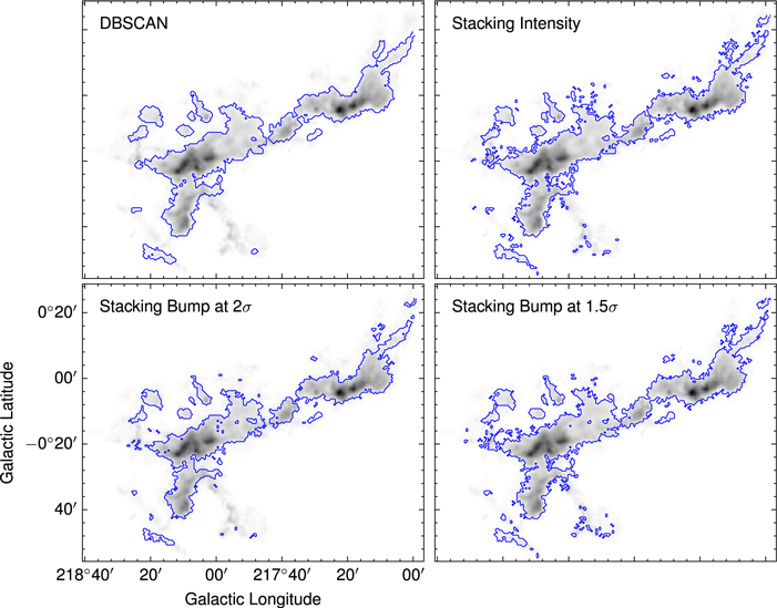
Figure 13. The spatial distribution of 13CO emission in cloud G217.383−00.083+026.19 (known as Sh 2–287; Gong et al. 2016) based on different algorithms. The background is the 12CO intensity, and the contour shows the boundary of 13CO emission.
Download figure:
Standard image High-resolution image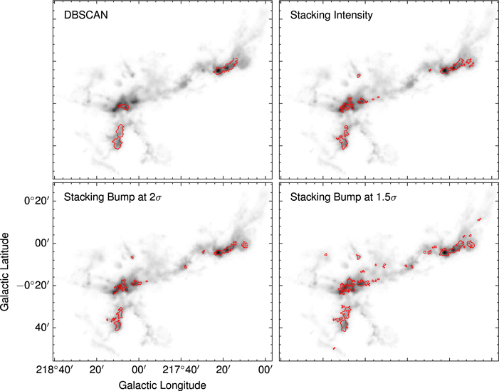
Figure 14. The spatial distribution of C18O emission in cloud G217.383−00.083+026.19 (known as Sh 2–287; Gong et al. 2016) based on different algorithms. The background is the 12CO intensity, and the contour shows the boundary of C18O emission.
Download figure:
Standard image High-resolution imageBy comparing the spatial distribution of 13CO and C18O emission identified by different algorithms, it is found that all the algorithms can find the main structure of 13CO and C18O emission, which means that there is no difference between these algorithms for detecting strong signals. The main difference among these algorithms is in the detection of weak signals. However, the stacking bump at 1.5σ algorithm shows the widest area of C18O emission. However, considering the false detections caused by spurious noise spikes (as discussed in Section 5.2), the weak signal identified by the stacking bump at 1.5σ algorithm partially comes from spurious noise spikes. Considering the accuracy and completeness of the algorithm, we prefer the stacking bump at 2σ algorithm.
5.4. Statistical Comparison of 13CO and C18O Emission
Figure 15 shows a statistical comparison of the number of pixels and the flux of clouds identified with 13CO signals under different algorithms, respectively. This indicates that in terms of the overall distribution, there is no significant difference in the 13CO flux value obtained among the three algorithms. It is obvious that the 13CO flux of each cloud searched by DBSCAN is systematically lower than the value obtained by the stacking bump at 2σ algorithm. There is no significant systematic bias in the number of pixels between the two algorithms in the clouds with large flux (12CO Flux > 1 × 10² K km s−1 arcmin2). This is due to the interception of data by DBSCAN based on the 2σ threshold when searching and calculating signals, which results in the loss of weak signals in each spectrum that are below the 2σ threshold. This effect is more significant in MCs with large pixel numbers.
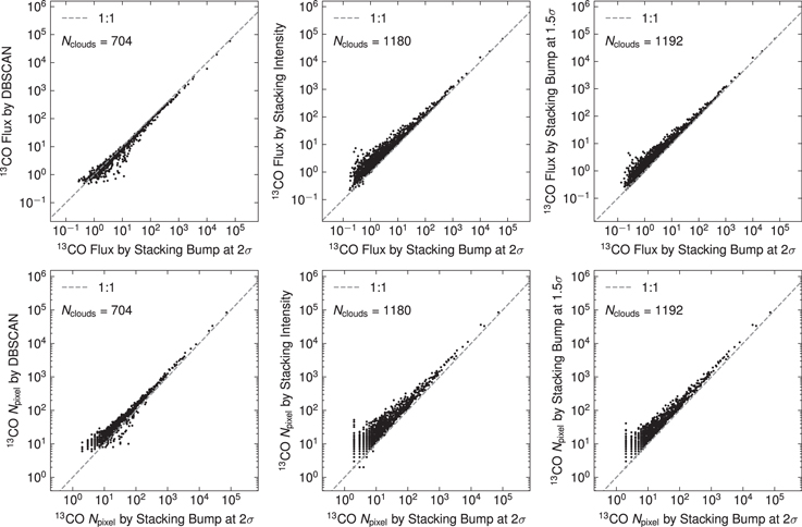
Figure 15. Statistical comparison of flux and pixel number of 13CO emission using different algorithms. The dotted line is the region where y = x. The number in the figure represents the number of signals that can be detected by both algorithms. The units of flux are K km s−1 arcmin2.
Download figure:
Standard image High-resolution imageThe pixel number and flux found by stacking intensity and stacking bump at 1.5σ are systematically higher than the results of the stacking bump at 2σ. As shown in the noise test results in Section 5.2, the systematic high results of the stacking intensity and stacking bump at 1.5σ algorithms may be caused by the noise injection after the threshold reduction. This indicates that blindly lowering the threshold may introduce too much noise into the statistics and lead to systematic bias in the results.
The comparison results of the C18O signals are similar to those of the 13CO signal (Figure 16). In the cross-sample between the DBSCAN algorithm and the stacking bump algorithm, the flux and pixel number obtained by the DBSCAN algorithm are systematically lower than those of the stacking bump algorithm, and the difference is stronger than that obtained by 13CO.
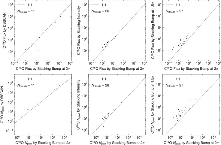
Figure 16. Statistical comparison of flux and pixel number of C18O emission using different algorithms. The dotted line is the region where y = x. The number in the figure represents the number of signals that can be detected by both algorithms. The units of flux are K km s−1 arcmin2.
Download figure:
Standard image High-resolution imageAs with the case of 13CO, the stacking bump algorithms are systematically biased in terms of flux and pixel number. As discussed above, this is caused by spurious noise spikes when lowering the threshold.
According to the above results, compared with the other two algorithms, the stacking bump at 2σ algorithm not only has a very low false signal detection rate in noise testing (Section 5.2) but also is better than DBSCAN in flux and spatial distribution. In a future study, we will focus on the results of the stacking bump algorithm.
5.5. Integral Range of C18O
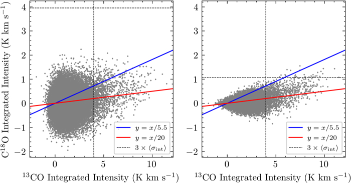
The integral range of 12CO is determined by the DBSCAN algorithm. Since the abundance of 13CO is lower than 12CO, its velocity range is generally slightly smaller than the 12CO range. Therefore, the approximation that the emission range in the 13CO spectrum is the same as 12CO can be a convenient way to determine the integration interval for 13CO. Even though noise will increase as the square root of the number of spectral channels in the integral interval, the difference in the velocity range between 12CO and 13CO is too small to produce a difference by orders of magnitude. However, this method is not suitable for C18O. The abundance of C18O is much lower than that of 12CO and 13CO; its velocity range is much smaller than the 12CO range. Hence, using the velocity range of the 12CO spectrum to integrate C18O is not a good idea; we try to integrate the C18O spectrum using the emission range of the 13CO spectrum.
Figure 17 shows the intensity distribution of cloud MWISP G217.942−02.083+034.45 by integrating C18O signals according to the velocity range within 12CO and 13CO emission regions (great than 2σ in the spectrum), respectively. This clearly shows that integrating C18O over the velocity range of 12CO will produce a large scattering, and the noise intensity is even greater than the signal intensity. If the C18O is integrated with the signal range of 13CO, the noise of the C18O integration intensity will be greatly reduced, which makes the signal easier to detect. Considering the influence of noise comprehensively, the integration of C18O in this paper is carried out in a range greater than the 2σ threshold in the 13CO spectrum.
Figure 17. The left panel shows 13CO vs. C18O integrated intensity of the cloud MWISP G217.942−02.083+034.45; the C18O intensity is integrated within the channels selected by the 12CO velocity distribution range pixel by pixel. The right panel also shows 13CO vs. C18O integrated intensity for the same cloud, but the C18O intensity is integrated with the channels selected by 13CO intensity greater than 2 × rms. The dashed lines represent the average value of triple integrated rms of 13CO and C18O, and the solid lines represent two typical ratios of 13CO to C18O in the cloud.
Download figure:
Standard image High-resolution image
6. Summary
We have shown 250 deg2 data in the 12CO, 13CO, and C18O (1−0) transitions of the third Galactic quadrant (195° < l <220°, ∣b∣ < 5°). An MC catalog containing complete information of 12CO, 13CO, and C18O has been constructed. The main conclusions are as follows:
- 1.A catalog of 7069 clouds has been built from the 12CO PPV datacube using DBSCAN algorithms.
- 2.Three algorithms, DBSCAN, stacking bump, and stacking intensity, are tested for the purpose of searching for 13CO and C18O signals within the PPV envelope of each 12CO cloud. The stacking bump algorithm is the most suitable algorithm for searching for 13CO and C18O signals in terms of detection rate. Under the stacking bump algorithm, a total of 1197 and 32 clouds were identified to have 13CO and C18O signals, respectively.
- 3.We test the stacking bump algorithm in the noise-only datacube and find that the 2σ threshold can effectively avoid the possibility of false detection generated by noise. The results proved that the new algorithm has high accuracy and completeness.
- 4.The detection rates of both 13CO and C18O increase steeply with parameters (peak intensity, projected area, and total flux) in cloud-by-cloud statistics. It is noticed that the percentage rate of C18O drops and stays between 50% and 80% when the 12CO peak value is greater than 24 K in pixel-by-pixel statistics.
- 5.Four velocity components are found in 12CO and 13CO velocity distribution, but only three of them are detected in C18O. Statistics of peak intensity, projected angular area, line width, and flux of the clouds show that the indices obtained by using different isotope probes are close to each other.
This research made use of the data from the Milky Way Imaging Scroll Painting (MWISP) project, which is a multiline survey in 12CO/13CO/C18O along the northern galactic plane with the PMO 13.7 m telescope. We are grateful to all the members of the MWISP working group, particularly the staff members at the PMO 13.7 m telescope, for their long-term support. MWISP was sponsored by the National Key R&D Program of China with grant 2017YFA0402701 and the CAS Key Research Program of Frontier Sciences with grant QYZDJ-SSW-SLH047. This work is supported by the Natural Science Foundation of Jiangsu Province (grant No. BK20201108). J.Y. is supported by the National Natural Science Foundation of China through grant 12041305. C.W. acknowledges the support by the Doctor Talents Program for entrepreneurship and innovation of Jiangsu province. This work is supported by the National Natural Science Foundation of China (grant No. 12073079). We also acknowledge the support by the Millimeter Wave Radio Astronomy Database (http://www.radioast.csdb.cn/). C.W. is grateful for the funding of the FAST Fellow. We would like to thank the referee for going through the paper carefully and much appreciate the many constructive comments that improved this paper.