


Abstract
When Mercury moves in its high-eccentricity orbit around the Sun, the background solar wind conditions are significantly changed. We investigated the effects of heliocentric distance and interplanetary magnetic field (IMF) orientation on the shape and location of Mercury's bow shock. We fit empirical models to the bow shock crossings obtained from the MErcury Surface, Space ENvironment, GEochemistry, and Ranging magnetometer observations under different conditions. Our results demonstrate that the bow shock moves antiplanetward when Mercury moves from perihelion to aphelion. However, this difference is not as significant as that of magnetopause due to the thickness variation of the magnetosheath. The IMF orientations show a weak influence on the bow shock shape and location, which implies that the southward magnetic field component is not the determinant factor that drives reconnection at the low-β magnetopause of Mercury.
Export citation and abstract BibTeX RIS

Original content from this work may be used under the terms of the Creative Commons Attribution 4.0 licence. Any further distribution of this work must maintain attribution to the author(s) and the title of the work, journal citation and DOI.
1. Introduction
Mercury is the closest planet to the Sun and has a large-eccentricity orbit. Since the Mariner 10 spacecraft first observed that the Mercury has a predominantly global dipolar intrinsic magnetic field, many interests have been attracted into this small magnetosphere of the planet (Baumjohann et al. 2006; Solomon et al. 2007). Mercury's intrinsic magnetic field resembles that of Earth in many aspects, but it is much weaker (less than 1% that of Earth; Ness et al. 1976; Anderson et al. 2010).
Due to the solar wind interaction with Mercury's magnetosphere, a bow shock and magnetopause are formed. The bow shock and the magnetopause can reflect the progress of solar wind–magnetosphere interaction (Russell et al. 1988; Slavin 2004; Slavin et al. 2019). Across the bow shock, the solar wind is compressed and deflected around the Mercury (Spreiter et al. 1966; Winslow et al. 2013). Theoretically, the bow shock shape and location are determined mainly by solar wind Mach number (MA ) and, to a less extent, interplanetary magnetic field (IMF) orientation (Spreiter et al. 1966; Slavin & Holzer 1981; Peredo et al. 1995; Winslow et al. 2013). Previous studies showed that the shape and location of magnetopause are principally affected by solar wind dynamic pressure, and the IMF orientation exerts influence on the shape and location of magnetopause due to magnetic reconnection-driven "erosion" of the dayside magnetosphere (Ferraro 1960; Slavin & Holzer 1979; Sibeck et al. 1991; Shue et al. 1998; Slavin et al. 2009a; Heyner et al. 2016; Jia et al. 2019).
Unlike the Earth, Mercury has a sizeable conducting core composed of liquid or molten metal (PEALE 1976). With solar wind dynamic pressure enhancements, the induction currents are driven at the top of Mercury's large iron core (Slavin et al. 2014; Jia et al. 2019). The induced magnetic fields act to limit and oppose the compression or expansion of the dayside magnetosphere by the solar wind (Suess & Goldstein 1979; Goldstein et al. 1981; Grosser et al. 2004; Glassmeier et al. 2007; Zhong et al. 2015).
Note that Mercury has a large-eccentricity ( ∼0.206) orbit with the perihelion of ∼0.307 au and the aphelion of ∼0.467 au. The background solar wind conditions from the perihelion to the aphelion are thus significantly different. James et al. (2017) examined the IMF properties and variations in Mercury's orbital zone. On the other hand, the interaction between the solar wind and the planetary magnetic field is different under different IMF orientations. Under northward IMF, the dominant effect is "compression." With solar wind dynamic pressure increasing, the compression effect grows significantly and leads to a planetward motion of magnetopause. A southward IMF component is supposed to facilitate magnetic reconnection, causing erosion on the dayside magnetosphere. However, DiBraccio et al. (2013) have demonstrated that the reconnection occurs for a wide range of magnetic shear angles, due to the low-plasma β around Mercury's environment. In addition, the low Alfven Mach number (MA ) and low-plasma β in Mercury's orbital region could influence both the rate and occurrence of magnetic reconnection, and the effect of reconnection is stronger at Mercury than that at Earth (Paschmann et al. 1979; Ding & Lee 1992; Scurry et al. 1994).
Using limited data obtained from Mariner 10, Russell (1977) modeled the shapes and locations of both the magnetopause and bow shock. After three flybys of MErcury Surface, Space ENvironment, GEochemistry, and Ranging (MESSENGER) spacecraft, Slavin et al. (2009b) updated these boundary shapes. Winslow et al. (2013) established the average shape and location of Mercury's magnetopause and bow shock using MESSENGER magnetic field data over a span of 3 Mercury years. They also found that shape shows no variation with the Alfven Mach number (MA ). Zhong et al. (2015) confirmed that the magnetopause standoff distance varies significantly over the course of the heliocentric distance during the 88 Earth days orbital period. Philpott et al. (2020) provided a complete list of bow-shock crossings with an estimation of their uncertainty. However, they did not resolve the effects of IMF orientation on the magnetopause or the bow shock. The shape and location of Mercury's bow shock vary with heliocentric distance has not been investigated.
In this paper, we establish the bow shock model of Mercury near perihelion and aphelion and under northward and southward IMF conditions by using the measurements from MESSENGER spacecraft. The objective of this work is to examine how the bow shock shape and location vary with heliocentric distance and how the IMF orientation affects those. We fit the empirical model to the bow shock crossings and build its shape. Based on our results, we demonstrate that the bow shock moves farther away from the planet's surface when Mercury moves from perihelion to aphelion. The effect of IMF orientation on shock shape and location is much weaker. Section 2 describes the magnetic field observations and how the boundaries were defined and built up the mean shapes of bow shock under different conditions. The results are given in Section 3, and how the bow shock shape and location respond to the heliocentric distance and IMF orientation is discussed in Section 4.
2. Method
After three flybys of Mercury following two of Venus and one of Earth, the MESSENGER spacecraft was inserted into Mercury's orbit on 18 March 2011 (Solomon et al. 2007). At first, the orbit about MESSENGER had a ∼12 h period, 82° inclination and high eccentricity. Subsequently, the orbit period was reduced to ∼8 hr on 2012 April 16. Our study uses MESSENGER magnetometer data from 2011 March 23 to 2015 April 30, neglecting those with high solar wind disturbance and some cases of which boundaries are difficult to be identified accurately. As clearly presented in Slavin et al. (2014), the bow shock noses under extreme solar wind conditions, such as the interplanetary coronal mass ejection (ICME) and high-speed stream, can be located significantly far away from the average location (Winslow et al. 2013) and thus affect the statistical results in this study. Finally, we conserved 3648 bow shock crossings.
Mercury's orbit has the highest eccentricity of all orbits of the planets in the Solar System and results in the distance from Mercury to the Sun ranging from about 0.30 to 0.47 au. The plasma and solar wind parameters are apparently sensitive to heliocentric distance. Thus, we classify all data into three different groups named "near", "mid," and "far" according to heliocentric distance to compare the difference of bow shock shapes between perihelion and aphelion. We do not choose distance-average classification because Mercury's orbital speed is faster at perihelion than that at aphelion. We set the interval near perihelion longer and that near aphelion shorter to make our samples have a relatively uniform distribution in number. The data distribution is shown in Figure 1. "Near" group consists of data during the period that Mercury is located between 0.30 au and 0.37 au and the "far" group consists of data during the period that Mercury is located between 0.42 au and 0.47 au. Other data are put into the "mid" group.
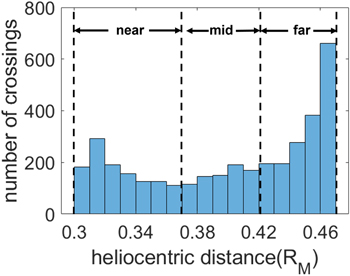
Figure 1. The distribution of bow-shock crossings with heliocentric distance. There are 1186 crossings in "near" group, 771 crossings in "mid" group, and 1691 crossings in "far" group.
Download figure:
Standard image High-resolution imageTo analyze the magnetic field data, Mercury solar orbital (MSO) coordinates are utilized, wherein the XMSO axis is positive sunward, ZMSO is positive northward, YMSO completes the right-handed system, and the origin of MSO coordinates is at the center of the planet. Considering the solar wind conditions and Mercury's orbital motion, the spacecraft data were transformed into an aberrated system. The aberration angle depends on solar wind velocity and the planetary-orbital velocity:
where vrevolution is the instantaneous velocity of the planet and vSW
is the solar wind speed. According to Winslow et al. (2013), the average aberration angle at Mercury is about 7° toward dawn. However, due to the variation of Mercury's orbital velocity between perihelion and aphelion, the aberration angle varies from 3 5 to 102. We set different values of aberration angle in different groups classified by the distance between Mercury and the Sun. In "near" groups, the aberration angle is set as 102. In "mid" and "far" groups, the aberration angles are set as 7° and 35, respectively.
Since the bow shock has a thickness of a few tens kilometers, the time position with a sharp increase near the solar wind is selected as the bow shock position. The thickness of bow shock is ignored. The inbound bow shock crossings were identified when the first steep increase in the magnetic magnitude ∣B∣ was observed. The outbound bow shock crossings were identified in the same manner as the magnetic field's last sharp decrease in magnitude ∣B∣. To make it clear, Figure 2 illustrates an example bow shock on 13 October 2012. The black vertical dashed lines denote the identified positions of the inbound and outbound bow-shock crossings. These criteria work well when the IMF has a ≥45° angle with the planet-Sun line. For quasiparallel shock crossings, the increment in ∣B∣ associated with the bow shock is less obvious.

Figure 2. (a) The observations from MESSENGER magnetometer for the first transit on 2012 October 13. The ordinate shows the scales for BX (in red), BY (in green), BZ (in blue) and ∣B∣ (in black). The vertical dashed lines denote the identified inbound and outbound crossings of the bow shock (in black) and magnetopause (in red). (b) Zoom-in view of the inbound bow shock crossing. (c) Zoom-in view of the outbound bow shock crossing.
Download figure:
Standard image High-resolution imageWinslow et al. (2013) have confirmed that the assumption regarding the boundaries as figures of revolution about the X axis is valid, so we make the same assumption. The northward offset of the planetary dipole is included in the definition of the distance from the axis of revolution, given by
where Zd = 0.196 RM (Anderson et al. 2011, 2012; Johnson et al. 2012).
To characterize the shapes of bow shock under different conditions, the data in each group are modeled by a conic section given by Slavin et al. (2009b):
where  . The focus point X0, the eccentricity
  , and the semilatus rectum L are determined by a nonlinear least-squares method.
3. Results
First, we use all crossings to fit the shape of the bow shock and show it in Figure 3. The dots are the crossings of bow shock we selected. The two curves are the results of Winslow et al. (2013; in yellow) and ours (in red). Our best-fit parameters are given in Table 1 and the bow shock subsolar distance is 1.98 RM , which is approximately equal to the results from Winslow et al. (2013), 1.90 RM . It can be seen that our model is similar to that of Winslow et al. (2013), but the shape of the bow shock in our work looks like sliding a short distance toward the Sun. This is mainly because Winslow et al. (2013) take the thickness of bow shock into account and use the mean value of the innermost and outermost edges as the bow shock position. However, we only picked the outermost bow-shock edges in our work.
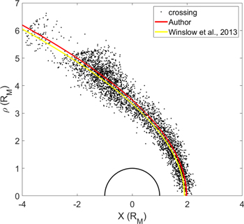
Figure 3. Scatter points are the inbound and outbound crossings of bow shock obtained from MESSENGER magnetometer. Curves show our best-fit result (in red) and the result from Winslow et al. (2013; in yellow).
Download figure:
Standard image High-resolution imageTable 1. Parameters of our Best-fit Model and the Study from Winslow et al. (2013)
| This study | Winslow et al. | |
|---|---|---|
|
| 1.036 | 1.04 |
| X0 | 0.5067 | 0.5 |
| L | 2.992 | 2.86 |
Download table as: ASCIITypeset image
Validated by comparing with the result from Winslow et al. (2013), this method is applied to investigate the difference in the shape and location of bow shock near perihelion and aphelion under northward IMF and southward IMF. As we can see in Figure 3, the crossings with XMSO > −2 RM are so scattered that, hereafter, we only conserve the crossings that XMSO ≥ −2 RM to reduce the fitting error. We first use data of "near", "mid," and "far" groups without regard to IMF orientation to fit the bow shock shapes. The results are shown in Figure 4 and the best-fit parameters are given in Table 2. In Figure 4(a), the thin pink curves are the trajectories of MESSENGER spacecraft located between 0.30 au and 0.37 au (same as the range of "near" group). The dots are bow shock crossings in the "near" group, and the red curve is the fitting result. Figures 4(b) and (c) are in the same format. We show the three fitted bow shock shapes in Figure 4(d) to get a better comparison. Because of the orbital resonance of MESSENGER spacecraft, the crossings in the three groups have different distributions, especially in the "mid" group. In Figure 4(b), fewer crossings are conserved in the "mid" group and are mainly scattered in two separate regions, which results in a very high fitting error. Subject to restrictions on MESSENGER spacecraft orbit, there are less or even no crossings near the subsolar point region in the "far" group. Crossings in the "near" group have the most uniform distribution. As it can be seen in Figure 4(d), the fitting shape of "mid" group is very different from that of "near" and "far" groups, so we will not discuss the results of the "mid" group in more detail hereafter. It can be found that the shapes of "near" and "far" are similar, but the nose of "near," with a subsolar standoff distance of 1.924 RM , is closer to the surface of Mercury than that of "far", with a subsolar standoff distance 2.1 RM . The movement of the bow-shock subsolar standoff point reaches 0.18 RM .

Figure 4. The trajectories of MESSENGER spacecraft from 2013 March 23 to 2015 April 30 are plotted in (a; in pink), (b; in light green), and (c; in light blue) according to the heliocentric distance of Mercury. The black dots are the crossings in "near", "mid," and "far" groups. The thicker curves denote our best-fit models in "near" group (in red), "mid" group (in green), and "far" group (in blue). All results are displayed in (d) for better comparison.
Download figure:
Standard image High-resolution imageTable 2. Parameters of Our Best-fit Models in "Near", "Mid," and "Far" Group without Regard for the Orientation of IMF
| Near | Mid | Far | |
|---|---|---|---|
|
| 1.092 | 0.8202 | 1.112 |
| X0 | 0.6104 | 0.0102 | 0.814 |
| L | 2.749 | 3.568 | 2.716 |
Download table as: ASCIITypeset image
Furthermore, we assess how the bow shock responds to the IMF orientation. The three groups mentioned above are classified by the IMF orientation. The IMF orientation is identified by taking the mean value of the 30 min of upstream IMF BZ . We present the bow shock shapes under northward and southward IMF conditions in Figure 5, and all parameters of our results are given in Table 3. The left and right panels are the results under northward IMF and southward IMF conditions, respectively. The dots are the crossings, and the solid lines are the fitting results near the perihelion (in red), and aphelion (in blue). The crossings have similar distribution under both IMF conditions. Under northward IMF conditions, the bow shock subsolar distance is 1.925 RM near perihelion and 2.031 RM near aphelion. The bow shock shapes look almost the same and slide a short distance of 0.106 RM when the Mercury moves from perihelion to aphelion in northward IMF. Under southward IMF conditions, the two shapes have more distinct differences, especially near the subsolar point region. The bow shock nose near aphelion (with subsolar distance 2.197 RM ) appears to move sunward from near perihelion (with subsolar distance 1.925 RM ) for 0.272 RM . Additionally, the two shapes under southward IMF conditions get closer in the nightside.

Figure 5. The dots are the crossings in "near" group (in pink) and "far" group (in light blue). Curves show our best-fit model in the "near" group (in red) and "far" group (in blue). The left panel (a) and right panel (b) display our best-fit models under northward IMF conditions and southward IMF conditions, respectively.
Download figure:
Standard image High-resolution image
Table 3. Parameters of Our Best-fit Models in "Near" and "Far" Groups with Regard to the IMF Orientation
| Northward IMF | Southward IMF | |||
|---|---|---|---|---|
| Near | Far | Near | Far | |
|
| 1.063 | 1.045 | 1.123 | 1.182 |
| X0 | 0.5623 | 0.554 | 0.664 | 1.123 |
| L | 2.812 | 3.018 | 2.678 | 2.334 |
Download table as: ASCIITypeset image
4. Discussions and Conclusions
We have constructed the Mercury's bow-shock time-average model by using the MESSENGER Magnetometer data from 2011 March 23 to 2015 April 30 (throughout the entire mission). Our models fitted by  are given by the parameter sets (X0 = 0.5067 RM
, = 1.036, L = 2.992 RM
, bow shock subsolar distance LBS
= 1.98 RM
) for the average bow shock, (X0 = 0.6104 RM
, = 1.092, L =2.749 RM
, LBS
= 1.924 RM
) for the bow shock near perihelion, and (X0 = 0.814 RM
, = 1.112, L = 2.716 RM
, LBS
= 2.1 RM
) for the bow shock near aphelion. The results of Winslow et al. (2013) and ours have little difference though different approaches are used to determine the bow shock locations. Winslow et al. (2013) identified the inner and outer limits of the boundary and took the midpoint of the limits as the bow-shock boundary. In this study, we only used the outermost boundary, because we focus on the bow shock differences under different conditions. The error caused by different approaches to determining bow-shock boundaries is negligible, and our method to identified the bow shock location is valid.
are given by the parameter sets (X0 = 0.5067 RM
, = 1.036, L = 2.992 RM
, bow shock subsolar distance LBS
= 1.98 RM
) for the average bow shock, (X0 = 0.6104 RM
, = 1.092, L =2.749 RM
, LBS
= 1.924 RM
) for the bow shock near perihelion, and (X0 = 0.814 RM
, = 1.112, L = 2.716 RM
, LBS
= 2.1 RM
) for the bow shock near aphelion. The results of Winslow et al. (2013) and ours have little difference though different approaches are used to determine the bow shock locations. Winslow et al. (2013) identified the inner and outer limits of the boundary and took the midpoint of the limits as the bow-shock boundary. In this study, we only used the outermost boundary, because we focus on the bow shock differences under different conditions. The error caused by different approaches to determining bow-shock boundaries is negligible, and our method to identified the bow shock location is valid.
To investigate the underlying effects of heliocentric distance on Mercury's bow shock, we classified the crossings according to the heliocentric distance into three groups named "near", "mid," and "far," and fit the empirical models to the data in each group. The parameter sets are given in Table 2. The crossings in the "mid" group are scattered in two separate regions, so the bow shock model for the "mid" group is not discussed. We find that the two shapes of bow shock near perihelion and aphelion have no significant difference, but in the subsolar region, the nose of bow shock has an outward motion of 0.18 RM from perihelion to aphelion.
The bow shock subsolar distance can be treated as
where LBS is the bow shock subsolar distance, LMP is the distance between the subsolar magnetopause and planet's center, while Dsheath is the subsolar thickness of magnetosheath. Theoretically, the magnetopause subsolar distance LMP is determined by the solar wind dynamic pressure Pdym, and the thickness of sheath Dsheath is determined by the solar wind Alfven Mach number MA . Note that under extreme solar wind conditions, the closeness of the bow shock to Mercury and the thinness of the magnetosheath could also be resulted from the direct solar wind impact on the planetary surface and at least partial absorption of the incident solar wind particles (Slavin et al. 2014).
Due to the lack of solar wind plasma observation from the MESSENGER spacecraft, the measurements from Parker Solar Probe are employed to provide the solar wind parameters in Mercury's orbital zone. Sun et al. (2022) showed the solar wind parameters, including convection electric field, dynamic pressure, plasma β, and Alfven Mach number as a function of heliocentric distances. According to their results, as Mercury moves from perihelion to aphelion, the solar wind dynamic pressure Pdym decreases and the Mach number MA increases. Therefore, from perihelion to aphelion, the decrement of Pdym leads to a increment in LMP because of the compression of magnetosphere (Zhong et al. 2015; Slavin et al. 2019); meanwhile, an increment of MA makes the thickness of magnetosheath thinner or a decrement in Dsheath (Spreiter & Stahara 1980). The derived distance of the bow shock from perihelion to aphelion in this study is 0.18 RM , which is smaller than that of the magnetopause, i.e., 0.27 RM as shown in Zhong et al. (2015). Such a result is consistent with the change of the magnetosheath thickness from perihelion to aphelion.
The bow shock changes its shape and location, to a lesser extent, with IMF orientation. All parameter sets are given in Table 3. Under northward IMF, the two bow shock shapes near perihelion and aphelion are similar with a short distance of 0.106 RM (Figure 5(a)). An underlying mechanism is that the induction currents limit the extant of expand of Mercury's magnetopause (Suess & Goldstein 1979; Goldstein et al. 1981; Grosser et al. 2004; Glassmeier et al. 2007; Zhong et al. 2015). Due to the effect of induction currents, the bow shock shapes have little difference when the planet is in northward IMF. Under southward IMF conditions, the two shapes are relatively different, and the distance between the two noses reaches 0.272 RM (Figure 5(b). With heliocentric distance increasing, the Alfven Mach number MA and plasma β increase (Slavin & Holzer 1981; Sun et al. 2022), which results in lower erosion efficiency at aphelion than at perihelion. Therefore, the planetward movement of bow shock is smaller when the Mercury is near the aphelion. On the other hand, Zhong et al. (2015) have demonstrated that the reconnection reduces the compressibility of magnetosphere. Therefore, we can deduce that the effect of magnetic reconnection is not predominated in southward IMF. However, due to the lack of upstream observations, the exact upstream solar wind conditions are unknown. Multiple-satellite observations from BepiColombo spacecraft in the future can help develop better bow-shock models of the Mercury.
This work is supported by the National Natural Science Foundation of China (NSFC) under grant 42122061, Macau Foundation, Project of Civil Aerospace "13th Five Year Plan" Preliminary Research in Space Science (D020308 and D020301), and the international partnership program of the Chinese Academy of Sciences under grant No. 183311KYSB20200017.