


Abstract
The hypothesis of the scale invariance of the macroscopic empty space, which intervenes through the cosmological constant, has led to new cosmological models. They show an accelerated cosmic expansion after the initial stages and satisfy several major cosmological tests. No unknown particles are needed. Developing the weak-field approximation, we find that the here-derived equation of motion corresponding to Newton's equation also contains a small outward acceleration term. Its order of magnitude is about  Newton's gravity (ϱ being the mean density of the system and
  the usual critical density). The new term is thus particularly significant for very low density systems. A modified virial theorem is derived and applied to clusters of galaxies. For the Coma Cluster and Abell 2029, the dynamical masses are about a factor of 5–10 smaller than in the standard case. This tends to leave no room for dark matter in these clusters. Then, the two-body problem is studied and an equation corresponding to the Binet equation is obtained. It implies some secular variations of the orbital parameters. The results are applied to the rotation curve of the outer layers of the Milky Way. Starting backward from the present rotation curve, we calculate the past evolution of the Galactic rotation and find that, in the early stages, it was steep and Keplerian. Thus, the flat rotation curves of galaxies appear as an age effect, a result consistent with recent observations of distant galaxies by Genzel et al. and Lang et al. Finally, in an appendix we also study the long-standing problem of the increase with age of the vertical velocity dispersion in the Galaxy. The observed increase appears to result from the new small acceleration term in the equation of the harmonic oscillator describing stellar motions around the Galactic plane. Thus, we tend to conclude that neither dark energy nor dark matter seems to be needed in the proposed theoretical context.
Export citation and abstract BibTeX RIS
1. Introduction: The Context
The problem of dark matter, noticeably raised decades ago by the dynamical studies of clusters of galaxies and by the flat rotation curves of galaxies, is still resistant to explanations. An impressive variety of exotic particles has been proposed in order to account for dark matter; see recent reviews by Bertone & Hooper (2017) and by de Swart et al. (2017). Simultaneously, theories of modified gravity like the MOND theory (Milgrom 1983) are not in arrears, as recently reviewed by Famaey & McGaugh (2012) and Kroupa (2012, 2015). In this interesting context, it may also be worthwhile to reconsider some basic physical invariances of the gravitation theory.
The group of invariances subtending theories plays a most fundamental role in physics (Dirac 1973). The Maxwell equations in absence of charge and currents are scale invariant, while the equations of general relativity (GR) do not enjoy this additional property (Bondi 1990). We know that a general scale invariance of the physical laws is prevented by the presence of matter, which defines scales of mass, time, and length (Feynman 1963). However, the empty space at large scales could have the property of scale invariance, since by definition there is nothing to define a scale. The real space is never empty in the universe; however, the properties of the empty space intervene through  , the Einstein cosmological constant. It is true that the vacuum at the quantum level is not scale invariant, since some units of mass, length, and time can be defined on the basis of the Planck constant. However, the large-scale empty space differs by an enormous factor from the quantum scales. Thus, in the same way that we may apply Einstein's theory at large scales even if we cannot do it at the quantum level, we may make the scientifically acceptable hypothesis that the properties of the empty space represented by
  at macroscopic and astronomical scales are scale invariant. In this work (see also Maeder 2017a, hereafter Paper I), we are exploring further consequences of the above hypothesis. The MOND theory has been noted to have this property (Milgrom 2009), but since this is a classical theory, it is not contained in a cosmological model.
The consequences are far reaching, as shown by the cosmological models in Paper I, which consistently include, through  , the invariance of the empty space at macroscopic scales. These models clearly account for the acceleration of the cosmic expansion, without calling for some unknown particles of any kinds. Several cosmological tests have been performed; they concern the distance versus redshift z relation, the magnitude–redshift m–z diagram, the plot of the density parameters
  versus
  , the relations of the Hubble constant H0 with the age of the universe and
  , the past expansion rates H(z) versus z and the transition from braking to acceleration, and more recently the past temperatures of the CMB versus redshifts (Maeder 2017b). All these tests are impressively satisfactory, and they open the possibility that the so-called dark energy may be an effect of the scale invariance of the empty space at large scales. Therefore, it is scientifically reasonable to explore further consequences of the above hypothesis to see whether at some stage it meets severe contradictions with the observations or whether it continues to show agreement. We now especially consider the dynamical evidences of dark matter.
As the internal dynamics of clusters of galaxies and the rotation of galaxies are at the origin of the claim for the existence of dark matter, we focus here on these dynamical problems. In Section 2, we study the Newtonian approximation of the geodesic equation consistent with the above key hypothesis. In Section 3, we examine the dynamical or virial masses of clusters of galaxies in the scale-invariant context and apply our results to the Coma Cluster and Abell 2029. In Section 4, we study the scale-invariant two-body problem and then discuss the outer rotation curve of the Galaxy. The case of galaxies at significant redshifts is also considered. Section 5 gives brief conclusions. In the Appendix, we examine the age–velocity dispersion relation of stellar groups in the Galaxy, in particular in the vertical direction where there is no consensus on the origin of the relation.
2. The Newtonian Approximation of the Scale-invariant Field Equations
2.1. Brief Recalls of Cotensor Analysis
To express the scale invariance of the empty space intervening through  at large scales, we must consistently do it in a theoretical framework that permits scale invariance (but does not necessarily demand it!). GR does not offer this possibility; however, a framework—the cotensor analysis—that allows it has been worked out in detail by Weyl (1923), Eddington (1923), Dirac (1973), and Canuto et al. (1977) (this was often in the context of the studies on variable G, but this is not what we do here). Short summaries of cotensor analysis are given by Dirac (1973) and in the Appendix of Canuto et al. (1977); see also Bouvier & Maeder (1978). In addition to the general covariance of tensor analysis used in GR, cotensor analysis also admits the possibility of scale invariance of the form

There,  is the line element in the GR framework with coordinates
  and
and  is the line element in a new more general framework, where we examine scale invariance. Parameter
  is the scale factor connecting the two line elements. If
  , the two frameworks are the same. In addition, we also make here a transformation of coordinates from
  to
to  , because we want to study simultaneously the effects of transformation of coordinates as in GR, together with the effects of a change of scale.
When the various steps of the development of cotensorial analysis are followed, a general scale-invariant field equation can be written (see Paper I). With respect to the usual field equation, it contains additional terms depending only on  and
and  , where

The term  is called the coefficient of metrical connection. It is as fundamental a quantity as are the
  in GR. The field equation is written as (Canuto et al. 1977)
The terms with a prime are those of GR. The gravitational constant G is a true constant, and  is the Einstein cosmological constant. A subscript ";" means a derivative. The application of the general field equation to the empty space has led in Paper I to some relations between the cosmological constant and the scale factor λ. The assumption is also made that the empty space is homogeneous and isotropic, which implies that scale factor λ is only a function of the cosmic time t. The 1, 2, 3 components (the three give the same result) and the 0 component of the above field equation become, respectively, for the empty space (Maeder & Bouvier 1979; Maeder 2017a)

The addition of these two equations gives  , the solution of which is

Here we keep the velocity of light c in the equations in order to write the weak-field equations with the appropriate units. From Equation (2), one also has  . This expression, together with Equation (4), leads to
which give the fundamental relations between  and the scale factor λ. We see that if
  , the scale factor would be a constant, that is to say, the scale-invariant framework would be strictly identical to GR. The first of the above equations leads to
  , where A is a constant. Taking
  at the present time t0, one has

The origin of time t depends on the cosmological models. For example, the numerical models in Paper I show that for  the origin lies at
  for a value of
  . This means that the variations of the scale factor λ are small, being limited to a change from 1.4938 at the big bang to 1.0 at the present time. For
  , one has
  and the variations of λ would go from infinity to zero. These examples show that the presence of matter rapidly reduces the cosmological effects of scale invariance (see Feynman 1963).
To study the dynamics of systems, we need an equation of motion. For that, we may derive the geodesic equation in the scale-invariant framework in various ways (Maeder & Bouvier 1979). Let us do it in a straightforward way, starting from the equivalence principle as expressed by Weinberg (1972). At every point of the spacetime, there is a local inertial system  such that the motion in GR may be described by

Let us develop this expression in the new framework (defined by ds2),


In cotensor analysis, scale-invariant derivatives of the first and second order have been developed preserving scale invariance. Other scale-invariant quantities are also defined; they are noted by an asterisk (Dirac 1973; Canuto et al. 1977). The modified form of the Christoffel symbol  corresponds to the first two derivatives in the second term on the left-hand side of Equation (10),

With Equations (2) and (11), we may write the equation of motion in the scale-invariant framework,

The modified Christoffel symbol is also written as (see relation (A5) by Canuto et al. (1977), relation (3.2) by Dirac (1973), or relation (86.3) by Eddington (1923))

Here,  is the usual Christoffel symbol, and the term
  is defined by Equation (2). Quite generally, as shown by the field equation, the scale-invariant terms are given by the corresponding usual terms in GR, plus or minus some functions of the
  and
and  . From relations (12) and (13), one has
The third and the last terms simplify, and one is left with the following geodesic equation:

with the velocity  . This equation allows one to study the motion of astronomical bodies for various conditions.
2.2. The Weak-field Approximation
The Robertson–Walker metric was used to derive the cosmological equations from the general field equations in Paper I. These equations were greatly simplified thanks to relations (6), which allow us to express  . Compared to the usual standard equations of cosmology, they only contain one additional term representing an acceleration opposed to gravity; see Equation (32) below. In view of Equation (7), the effects due to the evolution over a long period of time are expected to be the largest ones. The effects not depending on a time evolution are in principle the same as in GR.
Now, let us consider a test particle in the weak field of a potential Φ created by a central mass point. We now develop this nonrelativistic approximation, with  , of the geodesic Equation (15), which in the classical framework would lead to Newton's equation. The adopted metric only slightly deviates from the Minkowski metric,

This implies that the only nonzero component of the Christoffel symbols is (Tolman 1934)

We also have  , and the velocities are
  and
and  . The only nonzero component of the coefficient of metrical connection
  is
is  . Thus, the last term in Equation (15) vanishes. In the Newtonian-like approximation of the equation of motion, we have

In the cosmological models of Paper I, we have put c = 1, while this is not the case here. Also, since  is a function of time (see Equation (5)), we define, in order to avoid any ambiguity hereafter,

Thus, one has

We need to express the appropriate potential Φ. In the framework of GR, we would consider a central mass point  and examine the situation at a distance
  in a spherically symmetric system with a potential
  . In the scale-invariant system, from Equation (1) we have the correspondence
  . For the density, it is
  according to Equation (11) in Paper I. Thus,
  and the relation between the Einsteinian mass
  and the scale-invariant one is

The number of particles forming an object evidently does not change with time. Expression (21) is quite interesting: since the mass is changing like the length is doing, this means that the curvature of spacetime (or the gravitational potential) associated with a massive object is a scale-invariant quantity,

being the same in the GR and scale-invariant frameworks. Equation (18) applies to each of the i-components. In Cartesian coordinates we may write

In spherical coordinates, we can write the vectorial form of the equation of motion:

We recognize Newton's law plus an additional term opposed to gravity. This expression means that in addition to the curvature of space associated with a mass element, a particle may experience some outward acceleration associated with the nonconstancy of the scale factor λ. This additional term is generally very small, as discussed in Section 2.3.
We have to take the proper units of time in Equation (24). In current units, the present age t0 of the universe is 13.8 Gyr (Frieman et al. 2008) or 4.355 × 10¹⁷s. (This is an observed age value independent of cosmological models, resting essentially on the rather uncertain ages of globular clusters; see Catelan (2017) for a review. It is clear, however, that the relation between the age and a parameter like H0 depends on the cosmological models; see below.) The inverse of the above age is  s−1 or 70.85 km s−1 Mpc−1. Thus, the empirical value of
  is a quantity very close to the current value of the Hubble constant H0, which lies between 73 and 67 km s−1 Mpc−1 (Chen & Ratra 2011; Aubourg et al. 2015; Chen et al. 2016; Riess et al. 2016). We may write the relation between the Hubble constant and the age t0 of the universe in some chosen cosmological models as follows:

which may be written for other times with appropriate ξ. The numerical factor ξ depends on the cosmological model. For scale-invariant models with  and values of
  we have
  , respectively (see column (7) in Table 1 of Paper I).
Some developments of the weak-field approximation were already performed (Maeder & Bouvier 1979). However, at that time  was identified with the Hubble constant. Although the numerical values are very close to each other, there is an important physical difference between the two. The Hubble constant depends on the cosmological models, with
  being the result of the evolution of the universe for the appropriate parameters
  and
and  . This is physically different from the properties of the scale factor λ, which results from Equation (6).
Below, we shall carefully explore some first consequences of the above law of mechanics (24). Observations, rather than dogmas, will tell us whether the above modified Newton's law should be supported or rejected.
2.3. The Order of Magnitude of the New Term
Let us estimate numerically the relative importance of the additional acceleration term with respect to the Newtonian attraction at the present time t0. We consider a test particle orbiting with a circular velocity v at a distance r of a point mass M. The ratio x of the outward acceleration term resulting from the scale invariance of the empty space with respect to the Newtonian inward attraction term in Equation (24) is given by

We may now relate the present time t0 to H0 by expression (25) with the appropriate value of ξ, recalling that for the most realistic values of the density parameters  the value of ξ is of the order of unity. In turn, H0 may be related to the critical density of the universe at the present time. We have seen in Paper I that the true critical density
  corresponding to k = 0 in scale-invariant models is given by (see Equation (39) of Paper I)
Here,
is the standard critical density in Friedman's models. These densities are usually considered at the present time t0, but the above forms could also be used for other epochs with the appropriate H- and t-values. Now, the above x-ratio can be written in terms of the standard density  (the use of
  brings other expressions with no particular interest for the numerical estimates below),

Here, ρ is the mean density associated with the mass M within the radius r considered. (At a time t different from the present one, the corresponding values of the parameters need to be taken.) We will see, when studying the energy properties in Section 3.1, that the ratio  is not necessarily always equal to unity. As the dynamical evolution of a system proceeds, the additional acceleration term in Equation (24) may introduce progressive deviations from the classical relation
  . According to Section 3, the above ratio
  significantly differs from unity only for systems with a density within less than about 3 orders of magnitude from the critical density
  . Thus, we write
For systems with  , we may consider the equality in the above expression. The ratio x is thus mainly given by the ratio of the critical density to the average density of the dynamical system considered. We see that the dynamical effects of the scale invariance of the empty space are particularly significant in systems of very low density, such as clusters of galaxies and possibly galaxies.
The acceleration term would dominate over gravitation ( ) only for systems with ϱ smaller than about
  . The only such system known is the universe, which currently shows some cosmic acceleration. The matter density and the critical density have different time dependences. The matter density evolves according to the conservation law given by Equation (61) in Paper I, while the critical density varies like H2 (the variations of H(z) are given in Table 2 of Paper I for two useful models). The result is that the acceleration term dominates over braking only after a transition phase, which is located near z = 0.75 for models with
  and
and  (Maeder 2017a).
2.4. Consistency of the Modified Newton Equation and the Cosmological Equations
The scale-invariant cosmological models depend on the usual density parameters  and
and  , which now satisfy a relation of the form (see Equation (45) in Paper I)

For models with k = 0 supported by the observations of the CMB radiation (de Bernardis et al. 2000; Bennett et al. 2003), expansion implies  and thus
  with
with  . As in standard cosmology, from the two fundamental cosmological equations, a third one may be derived by elimination of the terms depending on the space curvature (Paper I); it is

Terms p and ϱ are the pressure and density in the scale-invariant system, respectively. R(t) is the expansion function. Taking p = 0 and considering that the density ϱ is the average density in a sphere of radius R and central mass M, we get

which compares with Equation (24). This shows the consistency of the above modified Newton equation with the scale-invariant cosmological equations in their limit.
Let us now consider the case of the empty space. In the Newtonian framework, a test particle would have a constant velocity with  . In the scale-invariant case, it would experience a slow acceleration. From the additional term in Equation (24) we have
  and thus
  . This is quite consistent with the results of Paper I, which show that the expansion function R(t) of an empty universe would behave like
  in the scale-invariant cosmology, while the empty Friedman model would expand like
  .
.
3. Dynamics of the Clusters of Galaxies
Clusters of galaxies play an essential role in the determinations of the cosmological parameters (Allen et al. 2011). Their distribution as a function of redshifts depends on the geometry of the universe and on the growth of density fluctuations, which both in turn depend on  and
and  (Frieman et al. 2008). The determination of the virial masses was the first applied method to obtain the mass of the clusters of galaxies (Karachantsev 1966; Rood et al. 1972; Bahcall 1974; Abell 1977; Blindert et al. 2004; Proctor et al. 2015). It was soon evident that the estimated virial masses were much too large compared to the visible mass in galaxies.
Specifically, we may consider that the stellar mass fraction  with respect to the total gravitational mass is of the order

There,  is the reference mass–luminosity ratio for a typical stellar population in galaxies and
  is the total gravitational mass–luminosity ratio determined for clusters of galaxies.
  is the total gravitational mass, also called the dynamical mass or virial mass, as it is determined on the basis of the virial theorem in standard Newtonian dynamics. The optical luminosity of galaxies originates mainly from stars, while the total gravitational mass is that of the baryons (stars, gas) and dark matter. From 600 groups and clusters of galaxies studied in various color bands, Proctor et al. (2015) supported values of
  for clusters with masses between 1014 and 1015
  . This compares well to most data by previous authors. For a typical stellar value of
  , one obtains
  –0.033, a value well supported by the recent works mentioned below.
Recent results from optical and X-ray observations of clusters of galaxies (Andreon 2010; Leauthaud et al. 2012; Lin et al. 2012; Gonzalez et al. 2013; Shan et al. 2015; Chiu et al. 2016; Ge et al. 2016) confirm that the stellar mass fraction  is quite small. Moreover, f* significantly decreases with increasing total mass (virial), typically from about 0.04 to less than 0.015 for clusters with masses from 1014 to 1015
  . Measurements of the X-ray-emitting gas provide estimates of the gas fraction
  , which largely dominates with respect to the stellar mass fraction f*. Results by the above authors also show that the gas mass fraction
  increases from about 0.08 to 0.15 over the above-mentioned mass interval. Clearly, most baryons reside in the hot gas. The baryon fraction
  , due to the opposite trends of the stellar and gas components, appears to be nearly constant with cluster mass (around 0.12–0.15; e.g., Gonzalez et al. 2013). However, this baryon fraction obtained from the addition of the stellar and gas components appears, according to the above authors, slightly lower than the cosmic WMAP 7 yr and Planck 2013 values of
  and 0.157, respectively. Whether this slight difference comes from uncertainties of the virial masses is a possibility (Chiu et al. 2016). The major fact is that the above baryon fraction
  is much lower than 1, by about a factor of 6. This is considered as strong evidence in favor of the existence of dark matter.
Now, we may wonder whether a part of the difference between the total gravitational mass and the baryonic mass could possibly originate from the scale-invariant dynamics.
3.1. Scale Invariance and the Virial Masses
We may not directly apply the virial theorem in the context of the scale-invariant theory, because of the additional term in Equation (24), which produces the expansion of a gravitational system (see Section 4.1). The additional radial outward acceleration term in Equation (24) may influence the relation between the motions and the present mass in a cluster of galaxies (Maeder 1978). We consider in a simplified way a spherical cluster containing N mass points of mass mi and velocity vi governed by the above modified Newton Equation (24). According to this equation, the acceleration of an object i interacting with another one of mass mj is

where rij is the distance between objects i and j and  according to Equation (19). Multiplying the above equation by
  , we get

This equation accounts for only one interaction i − j, and we have to sum up to account for all the gravitational interactions of the object i with the other masses mj in the cluster. Thus, we have

We now integrate the above differential equation. The system is nonconservative, because the additional outward acceleration term cannot be derived as the gradient of a potential. The non-Newtonian term is an "adiabatic invariant," since the rate of its effects is generally very slow. The usual treatment is to consider a limited but significant interval of time and to obtain relations between time averages. The integration of the above equation between time t1 and time tz, where z is the cluster redshift, gives
Let us take t1 as the time of the formation of the system. The effects of the nonconservative term in the initial collapse of the system are limited, and we have at equilibrium  . The above expression simplifies, and summing over all objects i, we get
In the above expression, there is a factor 1/2 in front of the double summation in order not to count twice the same interaction between a mass mi and the surrounding masses mj. We now take the mean over the N masses of the cluster considered to be spherical. The term on the left-hand side gives  , while the first term on the right-hand side of Equation (39) leads to
  , where R is the cluster radius and
  the mass determined in the scale-invariant theory. Here
  is an appropriate structural factor, which has no influence on the final result; see Equations (45) and (48). For the non-Newtonian term, we need to know how the velocities are varying with t. In an empty space,
  (Section 2.4), while in a bound two-body system the velocity is a constant (Section 4.1). Thus, we write
  , with β between 0 and 1. To express the last term in Equation (39), we define
The above-mentioned replacements lead to

The observed velocities are radial velocities, and we may write their relations to the total velocities

For isotropic motions of the galaxies within the cluster, we would have  and
and  , values that we adopt below. We finally write the expression corresponding to the virial theorem in the scale-invariant framework

This expression differs from the classical one by the parentheses on the left-hand side. The dynamical masses of clusters of galaxies published in the literature are based on the standard virial theorem. Some improvements in order to take into account the differences of the concentration of galaxies in clusters and other differences have been proposed (e.g., Rood 1974). The standard cluster masses  are based on a relation of the form

The ratio of the standard masses  from Equation (44) to the masses
  given by the scale-invariant theory in Equation (43) is equal to

Two protoclusters of galaxies in a forming stage have been observed at z = 5.7 (Ouchi et al. 2005). This corresponds to ages between 1.2 and 1.8 Gyr, for models with  between 0.3 and 0.1 for k = 0, giving an upper limit of
  . With
  , for
, for  , and 10, we have
  , and 100, respectively. With
  ,
,  rapidly diverges for
  . Thus, we may conclude that, except for clusters still in formation, the masses obtained by the standard virial theorem are often much larger than given by the scale-invariant theory.
Another estimate of F can be made by considering an average over an interval of time  equal to the radius crossing time
  , which often represents a large fraction of the cluster lifetime, especially when massive clusters are considered. This offers the advantage to provide an estimate based on observed parameters. We write
The intermediate time  is about
  . For f, we take 1 as for equilibrium (
 ). From Equation (39), we get

which leads to the following mass ratio for radial velocities with  :
:

This confirms that the masses derived in the present theory may be much smaller than the standard masses. A prediction of the theory is that forming clusters have little or no dark matter.
The ratio  of the mass to the luminosity of the observed clusters is considered in general. As the luminosities are essentially independent of the dynamical state of the clusters, we also have

The standard mass–luminosity ratios are also larger than those from the scale-invariant framework. There are uncertainties; nevertheless, these estimates confirm that some substantial part of the dark matter could be due to scale-invariant effects. As the dynamical masses have contributed to ascertaining the concept of dark matter, we now examine in two quantitative examples what fraction of the dark matter could possibly be due to the above effects.
3.2. The Case of the Coma Cluster and Abell 2029
The Coma Cluster and Abell 2029 are the most studied massive clusters of galaxies, and they both have about 1000 member galaxies. A recent study by Sohn et al. (2016) provides a very complete and detailed study of their luminosity, stellar mass, and velocity dispersion functions. For the Coma Cluster, they found a mass 
 and a radius
  Mpc (R200 and M200 indicate the values up to which the enclosed density is equal to 200 times the critical density). The velocity dispersion σ is 947 (±31) km s−1. For Abell 2029, the corresponding data are
 ,
,  Mpc, and
  (±31) km s−1. We point out that the radii R200 only encompass
  of the total volume of these clusters, which have observed total radii of about 6 Mpc, according to the data by Sohn et al. (2016). These authors have published the plot of the clustercentric velocities versus clustercentric distances for the Coma and Abell 2020 clusters. These plots support that the radial extension of these clusters reaches 6 Mpc.
For Coma the redshift is z = 0.0235, and for Abell 2029 it is z = 0.0784. According to the scale-invariant cosmological models with k = 0 and  –0.1 of Paper I, this corresponds to ages of about 13.5 and 12.8 Gyr, respectively (for these small z, different models make small differences). As for the radius crossing times, for more realistic radii of 5 or 6 Mpc, we get 5.16 or 6.20 Gyr (Coma) and 5.03 or 6.03 Gyr (Abell 2029), respectively. For the factor
  , we get
  . The corresponding estimates of the ratios
  in Equation (48) are

As a matter of fact, the above numerical values likely are not overestimated for two reasons. First, the above radii of 6 Mpc may still be too low. For example, in the case of Abell 2029, the concentration of points in Figure 5 of Sohn et al. (2016) may extend up to 8 Mpc. Second, in both clusters at large clustercentric distances the velocities are much smaller than in the cluster core. In Figures 5 and 6 of Sohn et al. (2016), the caustics defining the velocity limit decrease by about a factor of 2 from R200 to a distance of 6 Mpc. Even if the average velocity is reduced by 5% or 10%, this would significantly increase the ratios of the standard to the scale-invariant mass in both clusters. In fact, both the first and second effects intervene.
Thus, we see that the dynamical masses estimated in the scale-invariant system are smaller by a large factor (of about 4–12) with respect to the standard case. In this context, we recall that the baryon fraction from WMAP 7 yr and Planck 2013 turns around 0.16–0.17. Thus, with the above numerical figures, we see that there would be not much room, and maybe no room at all, left for dark matter in the context of the scale-invariant theory.
We conclude that a large fraction of the dark matter, and possibly the whole of it, is no longer demanded in the framework of the scale-invariant dynamics. More detailed analyses with extensive numerical simulations of the dynamical evolution of clusters of galaxies in the framework of the scale-invariant theory need to be performed in the future.
3.3. Mass Estimates in Relation to Cluster Density
We now examine the relation between the excesses of the standard masses (with respect to the scale-invariant results) and the average cluster densities. Expressing the term  with
with  (see Equation (25)) and the usual critical density
  , we get
where we have used Equation (44), also identifying the quadratic and arithmetic means of the velocities. According to Section 3.1, the critical density  must be taken at the redshift corresponding to tz. For the mass we take the standard mass
  ; thus, the density is the corresponding density
  of the cluster. The ratio
  may be written as

where, as seen above, we adopt  ,
,  . We see that the ratio of the standard to the scale-invariant masses increases for object of lower densities, consistently with the remarks in Section 2.3. For astronomical systems with densities much above the critical density of the universe, the two mass estimates are similar. Let us recall that Table 2 of Paper I allows one to estimate H and thus the critical densities at different redshifts.
Figure 1 shows the ratio  as a function of ratio of the cluster density
  with respect to the critical density at time tz. We see that the excess of the standard cluster masses with respect to the values in the scale-invariant theory rapidly diverges for values of the density ratio
  below 102, consistently with the results for the Coma Cluster and Abell 2029. Finally, we recall that, even within a given cluster, the standard estimates of the (M/L) ratio steeply increase for larger radii (Lewis et al. 2003), i.e., for decreasing average internal densities. This remarkable fact is quite in agreement with the above results and does not demand any peculiar distribution of dark matter according to clustercentric distances.
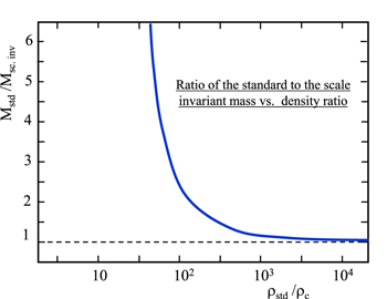
Figure 1. Ratio  as a function of the ratio of the standard density to the critical density, both considered at time tz of the cluster redshift z. This plot is based on Equation (52), with the values of the parameters indicated in the text. It also applies to the case of no or negligible redshifts.
Download figure:
Standard image High-resolution image4. The Rotation Curves of Galaxies
The flat curves of rotation velocities in the external regions of spiral galaxies usually provide another major evidence of dark matter; see review by Sofue & Rubin (2001) and further references in Section 4.2. The rotation velocities remain about constant instead of decreasing with central distance r, like  as predicted by the Newtonian law at some distance of an axisymmetric central mass concentration.
4.1. The Two-body Problem
We start by studying the classical case of the two-body problem in the scale-invariant framework, following some early developments by Maeder & Bouvier (1979). The specific angular momentum in the classical case is in Cartesian coordinates  , which is constant in time. Let us examine the product
  and its derivative,
Now, according to the expression of  in Equation (19), one has

Let us develop the two terms on the right-hand side of Equation (53),
In this last expression, the first and third terms on the right-hand side cancel each other, and the second and fourth terms are, according to Equation (23),


Now, we can write the complete expression
The two Newtonian terms cancel each other, and the same goes for the other terms. Thus, the above equation expresses the angular momentum conservation in the scale-invariant framework. The vector  is always orthogonal to the orbital motion, which indicates that the problem is two-dimensional. The angular momentum conservation is written in polar coordinates
  as
as

It is a scale-invariant term. At a fixed time, the above expression is similar to the usual conservation law. Now, the equation of motion (24) is written in the two polar coordinates as


The mass M is the mass in the scale-invariant framework; see expression (21). We easily verify the compatibility of expression (60) with the above Equation (62). The radial Equation (61) can be expressed with L,

We may transform the time derivatives into derivatives with respect to ϑ; with  we have
These replacements lead to an equation in  giving the curve described by a test particle in the central field of the scale-invariant mass. Most remarkably, the last term in the modified Newton Equation (63) simplifies with the last one in expression (64) for
  , and we have
This allows us with the transformation  to write

This expression is identical to the classical Binet equation except for the κ-term on the right-hand side. Thus, we may immediately write the solution  or
or

Here, r0 is the radius of a circular orbit (for e = 0). It is not a scale-invariant quantity. Recalling once more that the Einsteinian mass is  , we see that r0 grows like t, consistently with the basic relation (1). The eccentricity e is given by

We verify that the eccentricity e is scale invariant, which is satisfactory. The above Equation (67) is that of a conic, ellipse, parabola, or hyperbola depending on the eccentricity, however with a secular variation of the orbital radius r0, or semimajor axis as shown below.
The solutions of the two-body problem are similar to those of the standard case, with, in addition, slow secular variations of the orbital radius. More generally, if we consider the semimajor axis a of an orbital motion,

we have from Equations (67) and (69), together with Equations (7) and (19),

Thus, we see that the semimajor axis increases linearly with time t. The behavior of the circular velocity  is also interesting. From Equation (60) of the conservation of the angular momentum, we get

The constancy results from the fact that  behaves like
  and r0 like t, L being a constant. This is consistent with the fact that the gravitational potential is an invariant as shown by Equation (22). The constancy of the circular velocity over time is of great importance for the study of the rotation curves of galaxies below. From the conservation law (60), we also see that the orbital period P similarly varies like
  . This is also evident since the radius increases linearly and both the eccentricity and the circular velocity are constant.
Thus, the scale-invariant two-body problem leads essentially to the same solutions as the Newtonian case, with a slight supplementary outward expansion at a rate that is not far from the Hubble expansion. These conclusions consistently come from the hypothesis we have made (see Section 1). Now, whether this corresponds to nature or not can only be decided on the basis of careful comparisons with observations.
4.2. An Application to the Outer Rotation Curves of Galaxies
The rotation curves of nearby spiral galaxies, i.e., the circular velocities as a function of the galactocentric distances r, generally remain flat in the outer regions, instead of having a Keplerian decrease like  , as expected if most of the mass lies in inner regions. The velocity determinations are mainly based on optical observations of Hα, N ii, and S ii lines and on radio observations of H i and CO lines. There is a long history of the problem of the flat rotation curves, as reviewed by Sofue & Rubin (2001), who report that already in 1940 Oort noticed that "the distribution of mass [in NGC 3115] appears to bear no relation to that of the light." Such facts were further confirmed by other precursors. From a sample of 10 high-luminosity spiral galaxies, Rubin et al. (1978) stated that "all rotation curves are approximately flat, to a distance as great as r = 50 kpc." The sample was extended to 21 galaxies (Rubin et al. 1980), further supporting the previous conclusions. Nowadays, the observations of thousands of galaxies confirm the difference of the matter and luminosity distributions and support the existence of a halo of dark matter around the Milky Way and other galaxies (e.g., Persic et al. 1996; Sofue & Rubin 2001; Sofue 2012; Huang et al. 2016).
We concentrate on the case of the Milky Way where the rotation curve is known to the largest distances from the center. On the basis of the velocities of about 16,000 red clump giants in the outer disk, as well as ∼5700 halo K giants in the halo, Huang et al. (2016) have constructed the rotation curve of the Milky Way up to about 100 kpc. The average data as a function of the galactocentric distance are given in their Table 3, which indicates the various segments of the curve and the source of their measurements.
The curve by Huang et al. (2016) is illustrated in Figure 2; it shows a flat rotation curve with a circular velocity of 240 km s−1 up to galactocentric distances R of about 25–30 kpc and then slowly decreases down to 150 km s−1 at 100 kpc. There are also some prominent dips at R = 11 and 19 kpc (represented by the thin dashed red line in Figure 2). The error bars on the velocities are rather small ( km s−1) for R between 4.6 and about 13 kpc, so that the dip at 11 kpc appears as very significant. From R = 15 to 20 kpc, the error bars are much larger, so that the dip at 19 kpc may be less significant. Nevertheless, in view of the small amplitude of the dips with respect to the velocity, the rotation curve may be considered as globally flat up to at least 25 kpc (Huang et al. 2016). We note that the 11 kpc dip is often interpreted as due to a ring of dark matter at that location. The dip at 19 kpc may have the same origin; however, it could also be artificial owing to the use of different data sets. We note that Rubin et al. (1978) already pointed out secondary velocity undulations in various rotation curves, with rotational velocities lower by about 20 km s−1 on the inner edge than on the outer edges of spiral features.
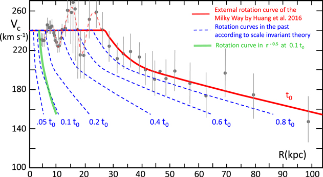
Figure 2. Evolution of the rotation curve of the Milky Way. The gray points are the observed velocity averages by Huang et al. (2016) with their error bars, and the thick red line represents the corresponding average rotation curve. The thin dashed red line describes the undulations in the globally flat part of the distribution. The blue broken lines show the rotation curves predicted by the scale-invariant theory for different past epochs expressed in a fraction of the present age t0. The thick green line shows a Keplerian curve in  at a time corresponding to 10% of the present age. We see that this Keplerian curve is close to a distribution consistent with the scale-invariant theory in an early epoch.
Download figure:
Standard image High-resolution imageThe decrease in the external regions reaches about 100 km s−1, which is about five times larger than the error bars. Moreover, it is supported by all measurements beyond a galactocentric distance  . The observed points then form a rather smoothly decreasing curve.
The red curve in Figure 2 is the velocity distribution at the present cosmic time t0. (In the cosmological models of Paper I, the present age is fixed to  , which corresponds to 13.8 Gyr. The correspondence between t0 and H0 is expressed by Equation (23) with the appropriate ξ-values.) We can find the corresponding velocity distributions at past epochs, 0.8 t0, 0.6 t0, 0.4 t0, etc., by applying the properties of Equations (70) and (71) derived from the equivalent Binet equation (Equation (66)) in the scale-invariant framework. At past epochs, the radii were smaller, while the circular velocities remained constant. Thus, we apply these simple evolution laws to the present rotation curve to deduce the curves at past epochs. Of course, this does not preclude the various dynamical effects that currently are at work in galaxies to be simultaneously operating: interactions due to spiral waves, effects of bars, nonaxisymmetric perturbations, radial motions, cloud collisions, mergers, etc. For now, we ignore these various effects in order to just examine the consequences of scale invariance.
Figure 2 shows that at earlier epochs the outer velocity distributions derived from the scale-invariant predictions were increasingly steeper with decreasing time. At the same time, the Galaxy was more compact. The galaxy formation occurred on a relatively short timescale compared to the age of the universe. At a given location, the infalling matter stops its collapse when the centrifugal force equilibrates gravity, thus establishing a Keplerian law. Later, during the aging of the Galaxy, the dynamical effects of scale invariance intervene, leading to a flatter distribution.
Let us consider that the initial Keplerian velocity distribution was of the form  , with the assumption of a relatively constant circular velocity
  up to a distance
  , followed beyond
  by a Keplerian decrease. As time progresses, the orbital radii increase by a factor of
  ; thus, at time t the velocity distribution becomes
We see that the scale transformation conserves the Keplerian law in  . As a matter of fact, the velocity distribution found by Huang et al. (2016) in the external regions of the Galaxy is close to a Keplerian law starting from
  . Consequently, the curve at past epochs, like
  , derived by a backward scaling from the present curve by Huang et al. (2016), is also close to a steep Keplerian distribution as shown in Figure 2.
Two important remarks need to be made. (1) There are a variety of rotation curves of galaxies as shown by Sofue & Rubin (2001). The available data generally concern radial extensions smaller than 20 or 30 kpc. Two very massive galaxies, UGC 2953 and UGC 2487, have been observed up to radial distances of 60 and 80 kpc, respectively (Sanders & Noordermeer 2007; Famaey & McGaugh 2012). Over these ranges, they only show a decline of 40–50 km s−1, smaller than the decrease of about 100 km s−1 for the Milky Way. However, these two galaxies are among the most massive and fastest-rotating galaxies, with maximum velocities of about 300 and 380 km s−1, respectively, much higher than in the Milky Way or in the galaxies studied by Sofue & Rubin (2001). Thus, it would be extremely interesting to know the rotation curves in the further outer layers of these extreme galaxies to see whether the decrease goes on, and whether their data can be interpreted in the context of the scale-invariant dynamics. (2) We also note that a remarkable correlation between the radial acceleration derived from the rotation curves and the distribution of baryons has been found (McGaugh et al. 2016; Lelli et al. 2017), implying that the dark matter is fully specified by the baryons. The obtained relation indicates the absence of dark matter at high acceleration and a systematic deviation for acceleration lower than about 10−10 m s−2. These findings that imply deviations from standard dynamics at the lower densities might provide further tests of the scale-invariant dynamics and will be studied in a future work (I am very indebted to the referee for these remarks).
Thus, we tend to conclude that the relatively flat rotation curves of spiral galaxies are an age effect from the mechanical laws, which account for the scale-invariant properties of the empty space at large scales. These laws predict that the circular velocities remain the same, while a very low expansion at a rate not far from the Hubble rate progressively extends the outer layers, increasing the radius of the Galaxy and decreasing its surface density like  when account is given to Equation (21). It is interesting that both the mass excesses derived from the virial in clusters of galaxies and from the flat rotation curves tend to find an explanation within the scale-invariant theory. In both cases, there is apparently no need of dark matter and unknown particles.
4.3. The Age Effect Derived from Genzel et al. (2017) and Lang et al. (2017)
The age effect in the rotation curves of galaxies is nicely confirmed by recent works by Genzel et al. (2017) and Lang et al. (2017). Six star-forming galaxies in the range  were studied in detail by Genzel et al. (2017), and a sample of 101 other galaxies between z = 0.6 and 2.6 were studied by Lang et al. (2017). The rotation curves they derive for these early objects show, with a high statistical significance, that the rotation velocities are not constant, but decrease in a compelling way with radius. They show that no dark matter is required to interpret the data, and the rotation curve is consistent with a pure baryonic disk. Even at a distance of several effective radii, the authors find that the dark matter fractions are modest or negligible, the results being essentially insensitive to the M/L ratios.
Figure 3 shows the stacked rotation curves with their error bars as derived by Lang et al. (2017). The points beyond the radius with maximum velocity show a decrease, which is not far from a  Keplerian curve (in green). Most of the galaxies of the sample are observed at epochs before the peak of star formation. This shows that the usual flatness of the rotation curve is a characteristic of the present epoch, but it is a property absent in the early stages. We emphasize that it is a bit worrying that the concentrations of dark matter, in the potential wells of which galaxies are supposed to form, are not present in epochs close to the formation time. Moreover, there is a progression in the presence of dark matter in spiral galaxies with time, since the observations by Wuyts et al. (2016) indicate that galaxies at z = 1 contain more dark matter than galaxies at z = 2, and in turn the local present galaxies show more dark matter than those at z = 1.

Figure 3. Stacked rotation curves with error bars from Lang et al. (2017) showing the normalized velocities vs. the normalized radii (i.e., the radii with respect to  , the radius where the maximum velocity is reached). The thick green line shows the Keplerian curve starting at the maximum velocity.
Download figure:
Standard image High-resolution imageIn Section 4.2, we have described a possible sequence in the dynamical evolution: cloud collapse–equilibrium–steep Keplerian velocity distribution–secular evolution according to Equations (70) and (71)–flatter rotation curve of galaxies. This scenario appears to account simultaneously for the observations of Genzel et al. (2017) and Lang et al. (2017), concerning the steep Keplerian rotation curve and the absence of dark matter at significant redshifts  , for the intermediate situation at medium redshifts
  (Wuyts et al. 2016), as well for the present flat rotation curves of most galaxies. These results appear to give some support to the above scale-invariant dynamics based on the modified Newton Equation (24).
Now, we may wonder whether the progressive flattening of the galaxy rotation curve is the only consequence of the scale-invariant stellar dynamics. As a matter of fact, the velocity dispersion, in particular in the so-called "vertical direction," shows a strong increase with age, known as the age–velocity dispersion relation (AVR; Seabroke & Gilmore 2007). This relation has received a variety of explanations over the past few decades without any clear consensus (see, e.g., Kroupa 2002; Kumamoto et al. 2017). The velocity dispersion in the Galactic plane is dominated by the effects of spiral waves, as well as by the collisions with giant molecular clouds that are strongly concentrated in the Galactic plane. However, in the directions orthogonal to the plane, there is little interaction since the stars spend most of their lifetimes out of the Galactic plane (Seabroke & Gilmore 2007). Thus, we may wonder whether the secular effects of scale invariance may play some role. The answer is positive; this problem is examined in the Appendix.
We also emphasize that the two problems of velocity dispersion and rotation curves are related. The vertical dispersion is an expression of the support in the vertical direction, while the rotation curves express the mechanical support in the horizontal direction. The results by Genzel et al. (2017) and Lang et al. (2017) show that the horizontal support is increasing with age, and the AVR shows a similar result for the vertical support. Thus, both mechanical supports of the Galaxy, vertical and horizontal, show an increasing trend with age.
5. Conclusions and Perspectives
There is progressively an accumulation of tests supporting the hypothesis of the scale invariance of the empty space at large scales; see also Milgrom (2009). First, there are the various cosmological tests (Maeder 2017a) mentioned in the introduction, as well as the test on the past CMB temperatures versus redshifts (Maeder 2017b). Now, the studies of the clusters of galaxies, of the rotation curves of the Milky Way and of high-redshift galaxies, and of the vertical velocity dispersion of stars in the Milky Way all appear positive. The long-standing problems of dark energy (Maeder 2017a) and dark matter may possibly find some solutions in terms of scale invariance. In this context, it is noteworthy that it has been claimed that halos of dark matter particles are inconsistent with a large variety of astronomical observations and in particular given the absence in the data of evidence for dynamical friction on the motions of galaxies due to these particles (Kroupa 2015).
These various results are encouraging, and the hope is that they will stimulate future works. The list of problems that await further studies is long. In this context, we again stress a central point of methodology: the tests, to be valuable, need to be internally coherent and not use "observations" implicitly involving in their derivations other cosmological models or mechanical laws.
I want to express my sincerest thanks to D. Gachet, R. Mardling, G. Meynet, and S. Udry for their support and encouragements.
Appendix: The Vertical Dispersion of Stellar Velocities in the Galaxy
We examine here the so-called problem of the AVR. This problem is in general not considered as an indication of dark matter; however, we shall see that it may provide another possible valuable indication about the effectiveness of scale-invariant dynamics. Three velocity components of the stellar velocities in the Galaxy are usually defined in stellar dynamics: component U toward the center, V in the direction of the Galactic rotation, and W orthogonal to the Galactic plane. The AVR problem is that of explaining why the velocity dispersion, in particular for the W-component, considerably increases with the age of the stars considered; see, for example, Seabroke & Gilmore (2007). Continuous processes, such as spiral waves, collisions with giant molecular clouds, etc., are active in the disk plane and may effectively influence the stellar velocity distributions. However, as emphasized by these authors, vertical heating (the increase of the dispersion  ) is unexpected, since stars spend most of their lifetime out of the Galactic plane. Thus, in order that they continuously receive some heating during their lifetime, there should be some heating process also active away from the Galactic plane.
The problem of the AVR and of the vertical heating already has a long history. A relation was first discovered by Stromberg (1946), in terms of a relation between velocities and stellar masses. It was further analyzed by Spitzer & Schwarzschild (1951), who studied the growth of the dispersion due to stellar collisions with giant molecular clouds, an effect also advocated by several followers. Seabroke & Gilmore (2007) performed a careful analysis of the extensive data set by Nordstrom et al. (2004) and examined the time behavior of the various heating processes. Their data points are given as blue triangles in Figure 4 showing the vertical dispersions as a function of age. Seabroke and Gilmore pointed out that the heating by giant molecular clouds should saturate after some time and that the dispersion would no longer increase. They give evidence that the vertical heating is continuous throughout the galaxy lifetime. Interestingly enough, they noticed the possible effect of a merger about 8 Gyr ago, visible as an outlier point in their figures (see also Figure 4). Among the other mechanisms considered, we may mention the heating by the gravitational field of spiral waves (Barbanis & Woltjer 1967; De Simone et al. 2004); by an unknown diffusive process (Wielen 1977); by massive halo black holes (Lacey & Ostriker 1985); by mergers of dwarf galaxies (Toth & Ostriker 1992); by the effects of evaporating star clusters (Kroupa 2002) when the star clusters that form expel their residual gas, causing the born stars to expand from the embedded cluster; and also by the effects of the evolution of the interstellar medium in the Galaxy as has been advocated by Kumamoto et al. (2017). As stated by these last authors, there is no consensus on the primary source of the AVR.

Figure 4. Vertical dispersion  as a function of the age of the stellar populations. The blue triangles with the error bars result from the analysis by Seabroke & Gilmore (2007) of the observations by Nordstrom et al. (2004). The solid red curve shows the predictions of the scale-invariant dynamics according to relation (77) for an age of the universe of 13.8 Gyr. The dashed red curve accounts for the fact that the Galaxy formed about 400 Myr after the big bang (Naoz et al. 2006). A vertical dispersion of 10 km s−1 is assumed at the present time.
Download figure:
Standard image High-resolution image
Let us study the effects of the scale invariance on the "vertical" velocity dispersion perpendicular to the Galactic plane following Magnenat et al. (1978). One may assume oscillations that are relatively small and far enough from the Galactic center. Thus, the potential perpendicular to the Galactic plane is separable, and the vertical force law Kz is linear in z. Taking the acceleration term as in Equation (23) into account, the equation of motion for the z-component becomes


Here, ϱ is the matter density in g cm−3 at the level of the Galactic plane. Care has to be given that  behaves like
  according to relation (21) and the preceding remarks. Thus, the oscillation periods increase linearly with time. The analytical solutions of Equation (73) for z and
  are
are


Here, the initial and present values have indices "in" and "0," respectively, and s is a number depending on the relative difference between the present age and the oscillation period. Equation (75) shows that the maximum amplitude  reached by a given star increases with the cosmic time. The velocity of a star born at a given time always keeps the same velocity
  when crossing orthogonally the Galactic plane. As a matter of fact, this (surprising) behavior of the velocity is consistent with the fact that both
  and the period of oscillation increase linearly with time. However, the constancy of the velocity of a given star does not mean that stars born at different times in the past (even if born at the same
  ) will have the same velocity at present time t0!
From Equation (76), the velocity  of a star born at
  , when crossing the plane (
 ), is given by

This applies at all times, and in particular at present. We may consider that the trend for the velocity dispersions follows that of the velocities. In agreement with the data by Seabroke & Gilmore (2007) shown in Figure 4, we take a value of 10 km s−1 for the present velocity dispersion  . Thus, as an example for a group of stars with a mean age of 10 Gyr, for an age of the universe of 13.8 Gyr the velocity dispersion is estimated to be about 10 km
  km s−1.
Figure 4 compares the corresponding model predictions obtained in this way (solid red curve) with the data from Seabroke & Gilmore (2007). We see that the theoretical curve well corresponds to the trend shown by the observations. We notice that in this plot two different sources of ages are intervening, on one side the ages from stellar evolution and on the other side the cosmic time t intervening in Equation (77). Despite this fact, the agreement is quite good, and the growth of the velocity dispersion  for the oldest stellar groups is well reproduced. In what precedes we have not accounted for the fact that a galaxy as massive as the Milky Way only forms when the universe is about 400 million years old (Naoz et al. 2006). Accounting for this delay in the star formation leads to the red dashed line in Figure 4, which even improves the overall agreement.
Not only the flat rotation curves of galaxies, which have been a strong argument in favor of dark matter, appear to be accounted for by the scale-invariant equivalent to Newton's law, but also the growth of the "vertical" velocity dispersion with the ages of the stellar groups in the Galaxy. This result appears consistent with the modified form of Newton's law, derived from the hypothesis of the scale invariance of the macroscopic empty space. This does not prove that it is right, but at least it shows the interest to pursue these kinds of studies.