


Abstract
The shapes of asteroid phase curves are influenced by the physical properties of asteroid surfaces. The variation of an asteroid's brightness as a function of the solar phase angle can tell us about surface properties such as grain size distribution, roughness, porosity, and composition. Phase curves are traditionally derived from photometric observations at visible wavelengths, but phase curves using infrared data can also provide useful information about an asteroid surface. Using photometric observations centered near ∼3.4 μm from the W1 band of the Near-Earth Object Wide-field Infrared Survey Explorer mission, we construct thermally and rotationally corrected infrared phase curves for a sample of main-belt asteroids, which includes asteroids observed by the AKARI satellite, as well as subsets of the Themis and Flora dynamical families. We calculate the linear slope of the phase curves as a measure of their shape and compare W1 phase slopes to band depths of absorption features associated with hydrated materials, spectral slopes, visible albedos, W1 albedos, and diameters. We observe a steepening of the W1 phase slope of C-type asteroids with increasing 2.7 μm band depth but little correlation between the phase slope and 3 μm band depth or 3 μm spectral slope. The C-types in our sample exhibit steeper average W1 phase slopes than M- or S-types, similar to visible-light phase slopes. We also observe steeper W1 phase slopes for smaller-diameter objects within the Themis family and explore comparisons to Jupiter-family comets in phase slope versus albedo space.
Export citation and abstract BibTeX RIS

Original content from this work may be used under the terms of the Creative Commons Attribution 4.0 licence. Any further distribution of this work must maintain attribution to the author(s) and the title of the work, journal citation and DOI.
1. Introduction
The shape of the phase curve of an asteroid is related to the physical properties of its surface, albeit in a complex way, including properties such as grain size, porosity, roughness, and composition (Belskaya & Shevchenko 2000; Muinonen et al. 2002; Oszkiewicz et al. 2011, 2012; Shevchenko et al. 2016). The relationship between the shape of the phase curve of an asteroid and its geometric albedo (referred to as "albedo" unless otherwise stated) is particularly interesting in visible light, as higher-albedo asteroids such as E-types (albedos > 0.3) exhibit flatter phase curves at phase angles larger than 10°, while lower-albedo asteroids like S-types (albedos between 0.1 and 0.2) or C-types (albedos < 0.1) show steeper phase curves as albedo decreases. These trends with albedo also correspond to the taxonomic type of an asteroid, which itself is an indicator of its surface composition (DeMeo et al. 2009). High-albedo E-type asteroids have more pronounced opposition effects and flatter phase curve slopes than low-albedo C-type asteroids. However, such relationships have yet to be explored using asteroid phase curves constructed from infrared photometry, specifically in the 3 μm region. Given the established links between the shape of a phase curve in visible light and the visible albedo and taxonomic type of an asteroid, the shape of a phase curve in the IR may also act as a probe of its surface properties.
While the shape of the phase curve of a given asteroid cannot conclusively identify a specific surface property of that asteroid (such as the presence of an individual substance), it can set reasonably strong constraints (Buratti et al. 2022), making the distribution of phase curve parameters within a group of asteroids a powerful tool. Comparing phase curves across asteroid families or spectral types can elucidate large-scale differences in composition or other surface properties. Oszkiewicz et al. (2012) explored the distribution of the G12 slope parameter across all asteroid families and found that some families exhibit homogeneity in G12 space, and in some cases G12 values can be indicative of taxonomic type. G12 is the slope parameter of the nonlinear H, G12 phase function, derived by Muinonen et al. (2010). Shevchenko et al. (2016) determined average G1 and G2 values for several taxonomic types, with low-albedo types exhibiting higher G1 values and lower G2 values than higher-albedo types. These slope parameters are from the H, G1, G2 phase function, also derived by Muinonen et al. (2010). Penttilä et al. (2016) introduced a set of one-parameter phase functions for various asteroid taxonomic types, and Oszkiewicz et al. (2021) provided average phase slope parameters for V-type asteroids. Additionally, Mahlke et al. (2021) used dual-band photometry from the ATLAS observatory to calculate G1 and G2 slope parameters for roughly 95,000 asteroids. Mahlke et al. (2021) concluded that the correlation of the G1 and G2 parameters with albedo would allow phase curves to be used as a proxy for albedo, while also finding that taxonomic complexes sufficiently separate in G1, G2 space to enable the study of ensembles of asteroids such as asteroid families. In conjunction with the results from Ďurech et al (2020), Mahlke et al. (2021) also found that phase curve parameters derived from the ATLAS data are band-dependent.
With these studies in mind, we turn our focus to an asteroid family of particular interest: the Themis dynamical family. This family is notable due to the discovery that several of its members exhibit volatiles on their surfaces (Rivkin & Emery 2010) or sublimating from their surfaces (Hsieh et al. 2004, 2010, 2011). This implies that the Themis family may be a reservoir of volatile material, making it an important focus for studies of volatile delivery to and within the inner solar system. Additionally, the Themis family is a substantial group of >4000 asteroids (Nesvornỳ et al 2015) with a large, well-studied parent body and a well-constrained age (Marzari et al. 1995; Nesvornỳ et al 2003), allowing for more precise tracing of family member history than many other main-belt objects. Given that the Themis family inhabits the outer region of the main belt, with most members having semimajor axes around 3 au (Nesvornỳ et al 2015), this places the Themis family at a crossroads between the inner and outer solar system as a large group of asteroids that may have played a key role in the eventual presence of volatile and organic material in the inner solar system.
The most reliable way to detect volatile and/or organic material is via reflectance spectroscopy. When considering asteroid surface composition, the 3 μm region is inherently interesting, as there are several substances believed to be important for the development of life that have spectral absorption features between 3 and 4 μm. These include many organic molecules (Moroz et al. 1998), ammoniated materials (Snodgrass et al. 2017), hydrated minerals, and water ice (Combe et al. 2016). Usui et al. (2019) published spectra of 66 asteroids (mostly from the main belt) using observations from the Japanese AKARI mission, which covered wavelengths from 2.5 to 5 μm. Their goal was to search for absorption features indicative of hydrated materials, which tend to have peak wavelengths around 2.7 and 3.1 μm. While spectra in this wavelength region are important for identifying such materials, they are not abundant in the literature, nor are they possible to obtain for many smaller asteroids. However, photometric observations in the 3 μm region do exist as a result of the Wide-field Infrared Survey Explorer (WISE) mission and its subsequent reactivation as the Near-Earth Object Wide-field Infrared Survery Explorer (NEOWISE). The WISE camera's W1 band covers wavelengths from roughly 3 to 4 μm, thus encompassing a region where organic and hydrated materials exhibit absorption features. While photometric data lack the detail needed to uniquely identify a particular substance, the presence of these materials should still have an impact on an asteroid phase curve. Thus, data from the WISE mission offer a unique opportunity to create phase curves using photometry in the 3 μm region.
In this study, we construct the first-ever asteroid phase curves using W1 photometry from the WISE/NEOWISE mission. We do this for a sample of asteroids that have existing 3 μm spectra from the AKARI mission, as well as for a sample of asteroids from the Themis dynamical family, a C-complex family. We also construct 3 μm phase curves for objects in the Flora family for comparison with the Themis family. In Section 2, we give an overview of the NEOWISE mission, its data products, and our data selection methods. We describe our process for constructing a phase curve from W1 photometry and subsequently estimating a W1 phase slope in the linear phase curve regime (phase angle > 10°) in Section 3. In Section 4, we present our results and compare the W1 phase slope distribution of AKARI asteroids with the asteroid spectral type, 2.7 μm band depth, 3.1 μm band depth, 3 μm spectral slope, albedo, and diameter, while also comparing the W1 phase slope of Themis-family asteroids with W1 albedo and diameter. Lastly, in Section 5, we discuss the viability of the W1 phase slope as a metric by which to identify the large-scale distribution of hydrated materials and organics in the inner solar system. We also explore an observed relationship between asteroid diameter and W1 phase slope, and we discuss potential similarities between Themis-family objects and Jupiter-family comets (JFCs).
2. WISE and NEOWISE: Overview and Data Products
The WISE mission was launched in 2009 and mapped the entire sky in four infrared bands centered at 3.4, 4.6, 12, and 22 μm (W1–W4, respectively) using a 40 cm telescope (Wright et al. 2010). The bandpasses are shown in Figure 1. After depleting its coolant in 2011, the mission was put into hibernation and then reactivated in 2013 as NEOWISE, observing only in the W1 and W2 bands. During the still-ongoing reactivation phase of the mission, NEOWISE has acquired over 1.4 million infrared measurements of 42,515 different solar system objects (as of 2023 March). Hereafter, we use "WISE" to refer to the spacecraft and "NEOWISE" to refer to the entire mission and its data products.
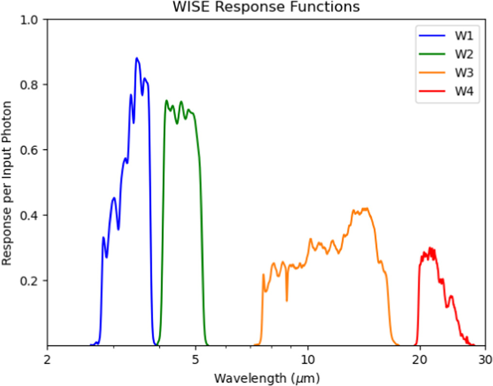
Figure 1. Filter response functions for WISE bandpasses. From left to right: W1, W2, W3, and W4. The W1 filter covers roughly the wavelengths from 3 to 4 μm.
Download figure:
Standard image High-resolution imageThe phase curves produced in this work cover a maximum range of ∼10°–15° in phase angle, with the minimum phase angle reached across all objects being ∼15° and the maximum being ∼35°, with some objects having as low as 5° of phase angle coverage. While ideal phase curves contain observations near 0° phase angle to characterize the opposition effect (Belskaya & Shevchenko 2000), such observations are not possible from NEOWISE due to the observing geometry of the WISE spacecraft. WISE is in a Sun-synchronous, circular, polar, geocentric orbit, meaning the solar elongation is kept constant at ∼90° (Wright et al. 2010). While this orbit allows for higher-quality observations of the ecliptic poles, it also vastly restricts the range of phase angles that are observable for main-belt asteroids with relatively stable semimajor axes. Despite this limitation, deriving the phase slope from the linear portion of an asteroid phase curve (>10°) still provides a meaningful characterization of the shape of the phase curve (Muinonen et al. 2022).
We extracted NEOWISE W1 photometric data from the publicly available NASA/IPAC Infrared Science Archive (IRSA) Single Exposure Source Database, which catalogs moving objects in conjunction with the Minor Planet Center to identify solar system objects in all images. IRSA sorts data by mission phase, of which there are four: WISE four-band (WISE Team 2020a), WISE three-band (WISE Team 2020b), WISE two-band (or WISE post-cyro; WISE Team 2020c), and NEOWISE reactivation (NEOWISE Team 2020), the latter two of which only observe in the W1 and W2 bands. Given an object identifier, we extracted all available W1 observations of that object in a given mission phase, including metadata associated with each observation, such as potential artifacts and photometric image quality. For each asteroid, we used these metadata in combination with the signal-to-noise ratio (S/N) for quality control to limit the number of outlying points included in our analysis. A summary of the flags and our imposed selection constraints is shown in Table 1. Additionally, we extracted the "w1mpro," "w1sigmpro," and "mjd" fields, which are the measured W1 magnitude, the error in the W1 magnitude, and the Modified Julian Date of the midpoint of the observation, respectively. Through JPL Horizons, 4 an online solar system data and ephemeris computation service, we used the time stamp to obtain the phase angle, heliocentric distance, and geocentric distance of the asteroid at the time of observation. The phase angle is needed for phase curve construction, while the heliocentric and geocentric distances are used to calculate the reduced magnitude. We also applied saturation corrections when appropriate, as given in Cutri et al. (2015). Saturation corrections are given as additive factors in magnitude space for the W1 bandpass in all mission phases. Object detections brighter than 9th magnitude required saturation correction, with the correction terms increasing with increasing brightness. For more information about saturation corrections, refer to II.1.c.iv.a. of the Explanatory Supplement to the NEOWISE Data Release Products 5 (Cutri et al. 2015).
Table 1. Summary of Flags Used to Filter Out Potentially Compromised Observations, as Well as the Constraints Implemented on Those Flags
| Flag | Description | Constraint |
|---|---|---|
| ph_qual | Photometric quality flag that provides a shorthand summary of the quality of the profile-fit photometry measurement in each band, as derived from the measurement S/N | A, B, or C (S/N > 2) |
| cc_flags | Contamination and confusion flag that indicates that the photometry and/or position measurements of a source may be contaminated or biased due to proximity to an image artifact | No cc_flags for W1 (value of 0) |
| w1rchi2 | Reduced χ2 of the W1 profile-fit photometry measurement | <10 |
| qual_frame | Frame quality score. The numerical net quality score that was assigned to the single-exposure frame set from which this entry was extracted by the QA process | >0 |
| moon_masked | Moon masking flag. Indicates if the single-exposure database frame set from which an entry was extracted falls within the area covered by the prior moon masks. These fixed-area masks denote regions contaminated by scattered light from the moon | No moon masking (value of 0) |
| saa_sep | SAA separation. The angular separation on the sky between the apparent position of WISE and the boundary of the South Atlantic Anomaly (SAA) at the time of observation for the frame set on which this entry was extracted | >5° |
| qi_fact | Frame image quality score. The numerical image quality score assigned to the single-exposure frame set from which this entry was extracted by the QA process | >0 |
| sso_flg | Solar system object association flag. A single-digit flag that indicates whether the source is positionally associated with the predicted position of a known asteroid, comet, planet, or planetary satellite at the time when this frame set was acquired by NEOWISE | Solar system object association (value of 1) |
| allwise_cntr | AllWISE Source Catalog association. Unique identifier of the closest source in the AllWISE Source Catalog that falls within 3'' of the position of this NEOWISE source | No WISE source within 3'' (value of null) |
| w1snr | W1 profile-fit measurement S/N. The ratio of the flux (w1flux) to the flux uncertainty (w1sigflux) in the W1 profile-fit photometry measurement | ≥7 |
Note. These constraints were imposed after extraction from the NASA/IPAC IRSA Single Exposure Source Database.
Download table as: ASCIITypeset image
3. Methodology
There are several steps to producing a W1 asteroid phase curve. This process included appropriate extraction and selection of data from the NEOWISE database (discussed in Section 2), estimation and removal of the thermal component of the observed flux in W1, proper application of color corrections, and correction for asteroid rotational modulation. Once a fully corrected phase curve was constructed, we were then able to fit for the W1 phase slope. Here we describe in detail the techniques employed to construct and evaluate a phase curve using W1 photometry.
3.1. Thermal Corrections
In order to construct accurate phase curves using W1-band photometry, we needed to remove the thermal flux component from the NEOWISE data and consider only reflected flux. To do this, we implemented a Near-Earth Asteroid Thermal Model (NEATM) to estimate the thermal flux in the W1 bandpass. The thermal contribution is expected to be minimal at W1 wavelengths at main-belt distances, but some asteroids required large thermal corrections (∼35% of the total observed flux) for observations at higher phase angles. We used methods based on those described in Harris (1998), Delbó & Harris (2002), and Mainzer et al. (2011a) to integrate the Planck function over the observer-facing hemisphere of an asteroid surface given a surface temperature distribution and phase angle. Equation (1) gives the expression for the NEATM model we implemented,
where  is the emissivity (assumed to be 0.9), R is the radius of the object, Δ is the object–observer distance, ϕ is an angle measured around the subobserver point such that ϕ = 0 at the subsolar point, θ is the angle from the subobserver point to a point on the asteroid such that θ equals α (the solar phase angle) at the subsolar point, and Bν
is the Planck function. The temperature distribution we used is given by Equation (2), where Tss
is the subsolar temperature and is given by Equation (3):
is the emissivity (assumed to be 0.9), R is the radius of the object, Δ is the object–observer distance, ϕ is an angle measured around the subobserver point such that ϕ = 0 at the subsolar point, θ is the angle from the subobserver point to a point on the asteroid such that θ equals α (the solar phase angle) at the subsolar point, and Bν
is the Planck function. The temperature distribution we used is given by Equation (2), where Tss
is the subsolar temperature and is given by Equation (3):


Here A is the Bond albedo, S is the solar flux incident on the asteroid, σ is the Stefan–Boltzmann constant, and η is the beaming parameter (∼1 for main-belt asteroids). The Bond albedo is determined using Equation (4),

where G is the H, G slope parameter (Bowell et al. 1989), assumed to be 0.15, as is convention unless a G parameter measurement is otherwise available. Δ and α were retrieved from JPL Horizons, while R, η, ρv , and G were retrieved from the published NEOWISE main-belt diameters and albedo data set available via the Planetary Data System Small Bodies Node (Mainzer et al. 2019). We calculated the expected thermal flux at the center of the W1 filter using the isophotal wavelength of 3.3526 μm given in Wright et al. (2010). We then multiplied the thermal flux estimate by the W1 filter response at the isophotal wavelength to obtain an estimate of the true amount of thermal flux observed through the W1 filter. We also applied color corrections to our estimates of the thermal flux, which are given in Table 1 in Wright et al. (2010) and depend on the bandpass and the effective temperature (Teff). We used Equation (9) from Mainzer et al. (2011a) to convert our calculation of Tss to Teff, then we interpolated between the Wright et al. (2010) blackbody color correction values for the W1 bandpass to determine the proper color correction for the given Teff of an object. The thermal flux was then multiplied by this color correction value, resulting in our final estimate of the thermal emission for an object.
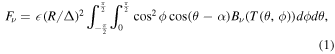
To obtain only the reflected flux, we converted the observed magnitudes to flux using the W1 zero-point (in Jy), also given by Wright et al. (2010), so that the thermal flux could be linearly subtracted off. We then applied one more color correction, again from Table 1 in Wright et al. (2010), for a G2V star observed in the W1 filter. This correction was applied only to the reflected-light estimate, since this light is reflected light from the Sun (a G2V star). We then converted the resulting flux value back to magnitudes to obtain a final estimate of the reflected light from a given asteroid in the W1 bandpass. This method of predicting and subtracting off the thermal flux resulted in estimates that varied as a function of phase angle, depicted in Figure 2.
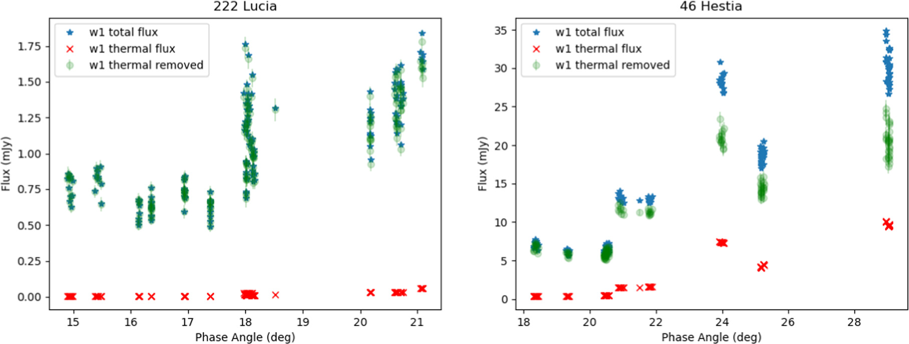
Figure 2. Left: raw observations of Themis-family asteroid (222) Lucia and the thermal flux estimates that were subtracted off. At most, the thermal flux accounted for roughly 4% of the total observed flux for (222) Lucia at the largest phase angles. Right: raw observations of C-type asteroid (46) Hestia, showing larger thermal flux contributions. Near 30°, the thermal flux accounted for roughly 35% of the total observed flux.
Download figure:
Standard image High-resolution imageThemis-family asteroid (222) Lucia was much less impacted by thermal flux removal than C-type asteroid (46) Hestia. However, (222) Lucia does not have observations at higher phase angles like (46) Hestia does, which is where the largest thermal corrections occur. It should also be noted that while thermal contributions to the observed flux can be significant, in most cases, the reflected-light component will be the dominant source of flux in W1. These two asteroids were chosen to illustrate the variation of the estimated thermal flux between objects.
3.2. Rotational Modulation
In addition to thermal corrections, we also must account for the rotational modulation of the brightness of each asteroid. Such corrections are necessary to ensure consistency among all phase curve data points, as brightness variations due to rotation may cause unnecessary spread in a resulting phase curve. The survey cadence of NEOWISE yielded an average of 10 detections over roughly 36 hr for a given solar system moving object (Mainzer et al. 2011b). These detections were close enough in time that there is minimal change in the phase angle, allowing us to treat these groups of observations as single lightcurves for the purpose of rotational correction. To compute and apply this correction, we employed a program called PerFit, which implements techniques outlined in Pravec et al. (2000), Kwiatkowski et al. (2009, 2010), and Wilawer et al. (2022). PerFit uses a combination of Fourier methods and least-squares fitting to determine the synodic rotation period of an asteroid based on its lightcurve. We employed a sixth-order Fourier series to fit the lightcurves, with the Fourier series given by Equation (5),
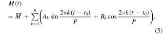
where  is the average brightness for a single lightcurve, Ak
and Bk
are the Fourier series coefficients, P is the synodic rotation period, t is the time of a given observation, and t0 is the time of the first observation in the lightcurve. To apply the correction, PerFit takes the average brightness of the lightcurve plus half of the peak-to-peak amplitude (obtained from fitting the Fourier series coefficients) to determine the maximum brightness of the asteroid. This maximum brightness is used as the point on the phase curve for the phase angle associated with the observing epoch of the input lightcurve. Thus, each asteroid lightcurve results in one point on the asteroid phase curve. Using the maximum brightness in this way is convention when constructing phase curves from rotationally modulated observations (Shevchenko et al. 2002).
is the average brightness for a single lightcurve, Ak
and Bk
are the Fourier series coefficients, P is the synodic rotation period, t is the time of a given observation, and t0 is the time of the first observation in the lightcurve. To apply the correction, PerFit takes the average brightness of the lightcurve plus half of the peak-to-peak amplitude (obtained from fitting the Fourier series coefficients) to determine the maximum brightness of the asteroid. This maximum brightness is used as the point on the phase curve for the phase angle associated with the observing epoch of the input lightcurve. Thus, each asteroid lightcurve results in one point on the asteroid phase curve. Using the maximum brightness in this way is convention when constructing phase curves from rotationally modulated observations (Shevchenko et al. 2002).
As an input to PerFit, we created composite lightcurves that consisted of a combination of NEOWISE W1 photometry and simulated V-band lightcurves based on shape models. Since NEOWISE data points are often too sparse to result in a well-populated W1 lightcurve, the incorporation of a dense, simulated V-band lightcurve allows for improved Fourier fits. The combination of W1 and V photometry is justifiable since rotational variations in brightness over the course of one rotation period are due to changes in reflected light rather than thermal emission. Since we removed the thermal emission component prior to correcting for rotational modulation, the W1 data at this point in the analysis are composed only of reflected sunlight. Observed flux in the W1 band is almost always dominated by reflected light rather than thermal emission, minimizing any rotational effects that would be a result of such emission. To create NEOWISE lightcurves, we selected an arbitrary threshold of 14 days between observations to be the cutoff between one lightcurve and the next. Thus, any observation within 14 days of a previous observation was incorporated into the same lightcurve. This ensured that W1 photometry included in a given lightcurve did not differ significantly in asteroid aspect or phase angle between data points. A summary of the aspect changes for all targets is shown in Table 2.
Table 2. Summary of Changes in Aspect for All Objects Included in This Work
| Object ID | Δ (au) | r (au) | α (deg) | λ (deg) | β (deg) |
|---|---|---|---|---|---|
| 5 | 0.01 | 0.075 | 0.218 | 1.88 | 0.057 |
| 6 | 0.003 | 0.021 | 0.157 | 0.607 | 0.235 |
| 7 | 0.013 | 0.068 | 0.283 | 2.376 | 0.323 |
| 8 | 0.01 | 0.072 | 0.213 | 2.498 | 0.342 |
| 10 | 0.001 | 0.019 | 0.125 | 0.247 | 0.03 |
| 16 | 0.004 | 0.061 | 0.145 | 1.229 | 0.099 |
| 21 | 0.002 | 0.022 | 0.181 | 0.617 | 0.044 |
| 24 | 0.005 | 0.092 | 0.583 | 0.773 | 0.022 |
| 33 | 0.005 | 0.022 | 0.161 | 0.764 | 0.015 |
| 42 | 0.01 | 0.077 | 0.531 | 1.037 | 0.273 |
| 43 | 0.003 | 0.02 | 0.205 | 0.762 | 0.067 |
| 44 | 0.003 | 0.019 | 0.166 | 0.486 | 0.044 |
| 46 | 0.007 | 0.07 | 0.652 | 2.297 | 0.122 |
| 62 | 0.006 | 0.051 | 0.146 | 0.818 | 0.02 |
| 79 | 0.009 | 0.082 | 0.183 | 2.326 | 0.176 |
| 89 | 0.016 | 0.123 | 0.868 | 2.907 | 1.046 |
| 90 | 0.006 | 0.062 | 0.136 | 0.72 | 0.018 |
| 129 | 0.01 | 0.143 | 0.152 | 3.707 | 1.017 |
| 145 | 0.007 | 0.07 | 0.188 | 1.499 | 0.413 |
| 173 | 0.019 | 0.112 | 0.305 | 1.468 | 0.191 |
| 216 | 0.003 | 0.055 | 0.118 | 0.498 | 0.13 |
| 222 | 0.005 | 0.05 | 0.156 | 0.722 | 0.062 |
| 246 | 0.006 | 0.077 | 0.161 | 1.283 | 0.469 |
| 281 | 0.007 | 0.094 | 0.685 | 1.744 | 0.268 |
| 341 | 0.003 | 0.058 | 0.229 | 3.099 | 0.118 |
| 352 | 0.003 | 0.021 | 0.214 | 0.685 | 0.056 |
| 364 | 0.008 | 0.075 | 0.692 | 1.555 | 0.427 |
| 383 | 0.006 | 0.108 | 0.153 | 1.724 | 0.113 |
| 419 | 0.003 | 0.057 | 0.154 | 0.674 | 0.079 |
| 461 | 0.006 | 0.068 | 0.107 | 1.137 | 0.039 |
| 468 | 0.008 | 0.088 | 0.288 | 1.911 | 0.006 |
| 492 | 0.003 | 0.057 | 0.425 | 0.427 | 0.034 |
| 526 | 0.004 | 0.056 | 0.162 | 0.632 | 0.018 |
| 540 | 0.001 | 0.017 | 0.214 | 0.456 | 0.09 |
| 553 | 0.011 | 0.093 | 0.636 | 2.451 | 0.369 |
| 561 | 0.001 | 0.019 | 0.112 | 0.272 | 0.012 |
| 621 | 0.006 | 0.053 | 0.148 | 0.649 | 0.064 |
| 700 | 0.002 | 0.018 | 0.199 | 0.426 | 0.071 |
| 704 | 0.005 | 0.13 | 0.792 | 0.619 | 0.867 |
| 710 | 0.005 | 0.052 | 0.381 | 0.43 | 0.03 |
| 767 | 0.002 | 0.022 | 0.118 | 0.346 | 0.018 |
| 800 | 0.012 | 0.12 | 0.208 | 6.052 | 0.321 |
| 802 | 0.005 | 0.068 | 0.204 | 1.937 | 0.275 |
| 841 | 0.004 | 0.061 | 0.198 | 1.486 | 0.166 |
| 905 | 0.008 | 0.069 | 0.269 | 1.7 | 0.307 |
| 936 | 0.012 | 0.091 | 0.151 | 0.972 | 0.065 |
| 946 | 0.005 | 0.062 | 0.151 | 0.702 | 0.028 |
| 951 | 0.003 | 0.019 | 0.215 | 0.678 | 0.073 |
| 956 | 0.013 | 0.107 | 0.233 | 1.678 | 0.159 |
| 996 | 0.002 | 0.018 | 0.13 | 0.262 | 0.006 |
| 1003 | 0.002 | 0.02 | 0.143 | 0.301 | 0.017 |
| 1047 | 0.014 | 0.081 | 0.247 | 2.077 | 0.288 |
| 1056 | 0.002 | 0.019 | 0.235 | 0.718 | 0.085 |
| 1058 | 0.011 | 0.073 | 0.749 | 1.572 | 0.146 |
| 1073 | 0.005 | 0.06 | 0.132 | 0.525 | 0.033 |
| 1082 | 0.008 | 0.071 | 0.12 | 1.413 | 0.083 |
| 1169 | 0.004 | 0.063 | 0.174 | 0.966 | 0.061 |
| 1188 | 0.006 | 0.051 | 0.199 | 2.212 | 0.312 |
| 1270 | 0.003 | 0.016 | 0.174 | 0.588 | 0.086 |
| 1365 | 0.005 | 0.056 | 0.576 | 0.554 | 0.216 |
| 1396 | 0.007 | 0.058 | 0.183 | 2.468 | 0.078 |
| 1419 | 0.007 | 0.059 | 0.202 | 1.91 | 0.092 |
| 1422 | 0.003 | 0.053 | 0.613 | 0.54 | 0.076 |
| 1446 | 0.006 | 0.11 | 0.236 | 1.849 | 0.219 |
| 1449 | 0.002 | 0.077 | 0.248 | 1.095 | 0.308 |
| 1514 | 0.016 | 0.104 | 0.746 | 3.319 | 0.111 |
| 1518 | 0.002 | 0.057 | 0.578 | 0.898 | 0.103 |
| 1523 | 0.009 | 0.102 | 0.174 | 2.228 | 0.352 |
| 1527 | 0.012 | 0.071 | 0.871 | 1.952 | 0.251 |
| 1576 | 0.008 | 0.073 | 0.149 | 0.831 | 0.008 |
| 1590 | 0.008 | 0.047 | 0.197 | 1.679 | 0.073 |
| 1608 | 0.01 | 0.065 | 0.182 | 2.052 | 0.251 |
| 1619 | 0.004 | 0.021 | 0.179 | 0.674 | 0.11 |
| 1623 | 0.002 | 0.019 | 0.117 | 0.342 | 0.019 |
| 1633 | 0.003 | 0.055 | 0.142 | 0.546 | 0.047 |
| 1636 | 0.006 | 0.056 | 0.191 | 1.098 | 0.143 |
| 1666 | 0.009 | 0.057 | 0.81 | 2.686 | 0.116 |
| 1667 | 0.01 | 0.076 | 0.406 | 1.899 | 0.162 |
| 1682 | 0.008 | 0.06 | 0.744 | 1.951 | 0.091 |
| 1687 | 0.007 | 0.056 | 0.148 | 0.714 | 0.069 |
| 1691 | 0.003 | 0.06 | 0.14 | 0.438 | 0.01 |
| 1733 | 0.005 | 0.057 | 0.794 | 1.502 | 0.2 |
| 1738 | 0.004 | 0.022 | 0.225 | 0.832 | 0.117 |
| 1752 | 0.011 | 0.089 | 0.212 | 2.788 | 0.123 |
| 1805 | 0.003 | 0.055 | 0.252 | 0.625 | 0.052 |
| 1820 | 0.012 | 0.058 | 0.865 | 3.057 | 0.379 |
| 1850 | 0.002 | 0.104 | 0.184 | 3.634 | 0.302 |
| 1997 | 0.015 | 0.08 | 0.637 | 2.354 | 0.224 |
| 2058 | 0.002 | 0.017 | 0.126 | 0.28 | 0.018 |
| 2094 | 0.002 | 0.017 | 0.199 | 0.477 | 0.06 |
| 2163 | 0.005 | 0.068 | 0.4 | 0.548 | 0.036 |
| 2165 | 0.002 | 0.068 | 0.165 | 0.42 | 0.008 |
| 2217 | 0.006 | 0.092 | 0.53 | 1.734 | 0.04 |
| 2248 | 0.005 | 0.064 | 0.198 | 0.867 | 0.036 |
| 2264 | 0.007 | 0.066 | 0.503 | 1.412 | 0.005 |
| 2372 | 0.002 | 0.019 | 0.109 | 0.354 | 0.025 |
| 2399 | 0.003 | 0.049 | 0.785 | 1.368 | 0.337 |
| 2404 | 0.002 | 0.043 | 0.112 | 0.348 | 0.025 |
| 2510 | 0.013 | 0.052 | 0.204 | 1.368 | 0.067 |
| 2534 | 0.002 | 0.018 | 0.125 | 0.349 | 0.006 |
| 2659 | 0.003 | 0.137 | 0.116 | 1.299 | 0.029 |
| 2708 | 0.002 | 0.017 | 0.16 | 0.272 | 0.029 |
| 2718 | 0.005 | 0.049 | 0.505 | 0.358 | 0.036 |
| 2803 | 0.002 | 0.02 | 0.146 | 0.302 | 0.009 |
| 2839 | 0.01 | 0.076 | 0.221 | 1.931 | 0.182 |
| 2874 | 0.002 | 0.019 | 0.185 | 0.601 | 0.077 |
| 2882 | 0.003 | 0.021 | 0.143 | 0.344 | 0.003 |
| 2896 | 0.017 | 0.106 | 0.282 | 3.193 | 0.508 |
| 3272 | 0.002 | 0.062 | 0.194 | 1.901 | 0.212 |
| 3301 | 0.007 | 0.07 | 0.563 | 1.785 | 0.219 |
| 3493 | 0.003 | 0.062 | 0.222 | 1.265 | 0.122 |
| 3749 | 0.007 | 0.071 | 0.202 | 1.694 | 0.219 |
| 3813 | 0.003 | 0.016 | 0.217 | 0.584 | 0.075 |
| 3831 | 0.013 | 0.052 | 0.238 | 1.902 | 0.275 |
| 3899 | 0.006 | 0.052 | 0.154 | 0.769 | 0.066 |
| 4012 | 0.003 | 0.018 | 0.213 | 0.711 | 0.077 |
| 4488 | 0.007 | 0.072 | 0.239 | 2.621 | 0.067 |
| 4570 | 0.002 | 0.017 | 0.222 | 0.584 | 0.077 |
| 4912 | 0.008 | 0.073 | 0.233 | 1.758 | 0.07 |
| 5069 | 0.004 | 0.06 | 0.16 | 2.274 | 0.134 |
| 5714 | 0.002 | 0.019 | 0.135 | 0.42 | 0.008 |
| 7043 | 0.003 | 0.02 | 0.249 | 0.866 | 0.074 |
| 7898 | 0.003 | 0.014 | 0.18 | 0.734 | 0.079 |
| 14257 | 0.004 | 0.059 | 0.175 | 2.19 | 0.319 |
Note. Δ is the heliocentric distance, r is the observer distance, α is the phase angle, β is the observercentric (in this case geocentric) ecliptic latitude, and λ is the observercentric ecliptic longitude. These values represent the maximum change in each parameter across all lightcurves constructed for a given asteroid. For example, asteroid (5) Astraea has an α value of 0.218. This means that for all lightcurves constructed for (5) Astraea, the largest change in phase angle in any single lightcurve was 0 218.
218.
Once parsed in this way, the NEOWISE lightcurves were combined with the simulated visible lightcurves. The simulated lightcurves were obtained from the Interactive Service for Asteroid Models (ISAM; Marciniak et al. 2012). ISAM is a web service dedicated to the representation of physical ephemerides of asteroid shape models. The tool has several functionalities, but the most useful for this work was its ability to generate simulated lightcurves at a given observing epoch using asteroid shape models from Ďurech et al (2010). Generating synthetic lightcurves in this way accounts for any changes in asteroid aspect or observing geometry between observing epochs.
Figure 3 shows an example composite lightcurve for asteroid (222) Lucia. Upon initial construction of the composite lightcurves, many showed significant shifts in rotational phase between the W1 lightcurves and the simulated V-band lightcurves. This is partly explained by the epochs of the shape model used to simulate the V-band lightcurves compared to those of the W1 observations. For objects with older shape model epochs, small errors in the rotation period propagate over the length of time between that epoch and the time for which the lightcurve is simulated. This lightcurve is simulated to match observations made in 2010, but the epoch of the shape model for (222) Lucia is in 1977. To account for this, we applied a cross-correlation to determine the shift in rotation phase between the W1 lightcurve and the V-band lightcurve. We then adjusted the lightcurves by converting the shift in rotation phase to an offset in Julian Date and applying this offset to the input W1 lightcurves. However, it should be noted that since the fitting procedure uses the maximum brightness of the lightcurve to determine the rotationally corrected phase curve data point, horizontal shifting between the two lightcurves in rotation phase space has a minimal impact on the resulting phase curves and therefore does not significantly impact our results.
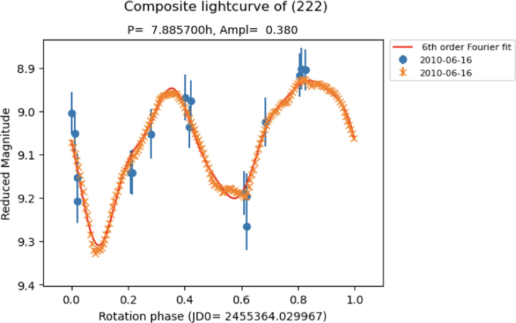
Figure 3. Composite lightcurve of asteroid (222) Lucia, a member of the Themis dynamical family. Orange points are the simulated V-band lightcurve from ISAM, while blue points are W1 observations from NEOWISE. The red line is a sixth-order Fourier fit used to estimate the synodic rotation period and determine the rotation correction.
Download figure:
Standard image High-resolution imageOnce PerFit creates a composite lightcurve and fits for the rotation period, the output is the reduced magnitude of the object at a particular solar phase angle at the given observing epoch. Each individual point in our phase curves is derived from thermally corrected composite lightcurves, which are then corrected for rotation and normalized by their geocentric and heliocentric distances at the time of W1 observations. In other words, each composite lightcurve is reduced to a single point on the phase curve, where that point represents the maximum brightness of the input lightcurve. For more details, see Wilawer et al. (2022).
3.3. W1 Phase Slope Calculations
After the necessary corrections were applied and the phase curves were constructed, we calculated the linear slope of the phase curve for each object. Since the only phase angles achievable by the WISE spacecraft for main-belt objects lie outside the nonlinear phase curve regime (>10°), we treated our phase curves as linear. We utilized linear least-squares regression to determine the best-fit slope to the data for each object, as these simple fits were sufficient to quantify the shape of the phase curve in the linear regime. We elected not to implement more complex fitting routines (e.g., H, G or H, G12 fitting) given the restricted range of phase angles covered by NEOWISE data, including the lack of observations at phase angles that would cover the opposition effect. In order to determine the goodness of fit, we utilized a Wald test and the coefficient of determination. The Wald test was employed with an alternative hypothesis that the slope of the regression line was negative. Since negative phase slopes are unphysical, a p-value of >0.05 was taken to represent a positive slope and thus an acceptable fit. The coefficient of determination was used to further assess the quality of our fitting, as we employed a threshold of >0.2 to represent a reasonable fit. Any objects returning p-values of <0.05 or coefficients of determination of <0.2 were removed from our sample. Additionally, we imposed a minimum phase angle coverage of 4° and a minimum number of seven phase curve points, with the intent of avoiding erroneous phase slopes resulting from fitting over a small range of phase angles or fitting a small number of points.
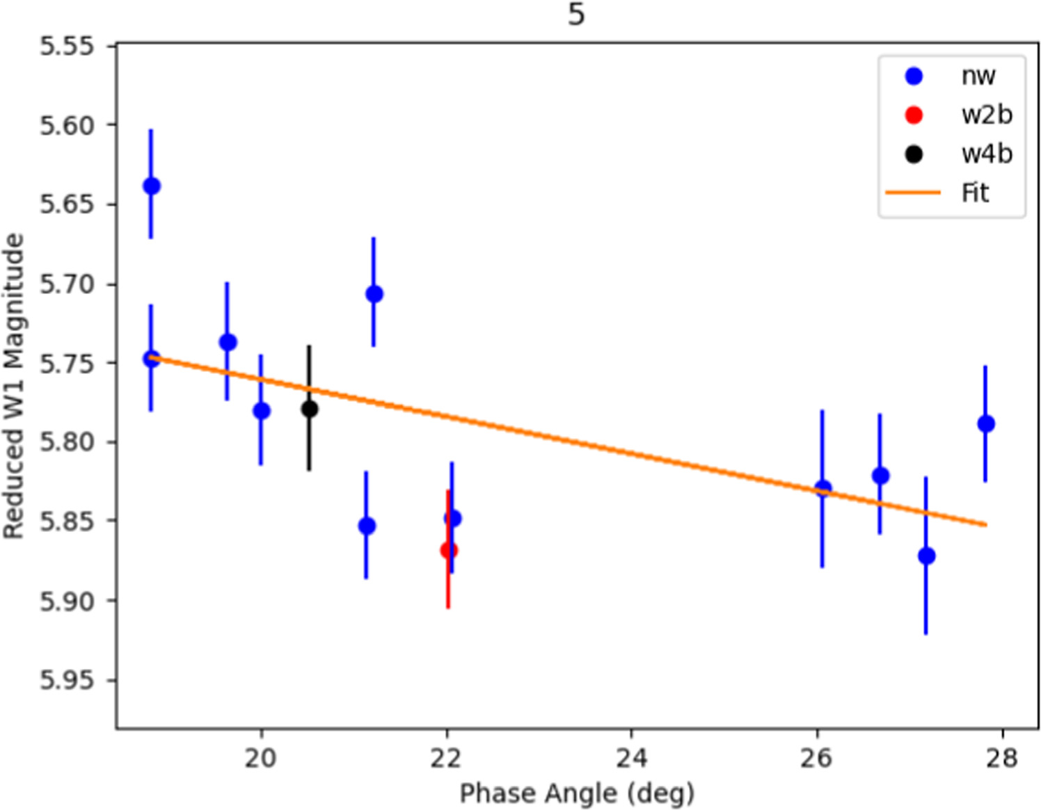
As a representative example, Figure 4 shows a fully corrected final phase curve for asteroid (222) Lucia. This particular object only has NEOWISE data spanning roughly 6° in phase angle, yet we are still able to discern the expected phase curve shape. Phase curves for the entirety of our sample are included in the Figure 14 in the Appendix.
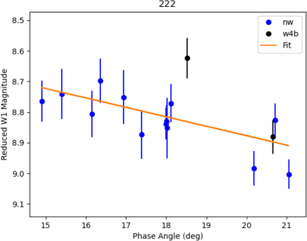
Figure 4. W1 phase curve of (222) Lucia. This phase curve was produced using thermally and rotationally corrected observations from all phases of the NEOWISE mission. Blue points use observations from the reactivation phase, while the black points are from the four-band, full cryo phase of the mission. The orange line is the linear fit from which a slope is derived.
Download figure:
Standard image High-resolution image4. Results
Here we present the results of our W1 phase slope analyses. We compare the W1 phase slope of asteroids from the AKARI sample with their visible albedos, 2.7 μm band depths, 3.1 μm band depths, and 3 μm spectral slopes. We also compare the W1 phase slope of Themis family member asteroids with their W1 albedos and diameters, which are determined using methods from Masiero et al. (2011). We display all phase slopes in units of reduced magnitude/radian; however, we show all phase curves (e.g in Figures 4 and 14) as reduced magnitude versus phase angle in degrees, since most phase curves are shown in this manner. All W1 albedos, visible albedos, and diameters were obtained from Mainzer et al. (2019), while all band depths and spectral slopes were measured by Usui et al. (2019). A summary of the observations used and the final derived W1 phase slopes for all objects is shown in Table 3.
Table 3. A Summary of the Observations Used and the Derived Phase Slopes for All Objects in This Work
| Object ID | No. of NEOWISE Obs. |
 (deg) (deg) |
 (deg) (deg) | W1 Phase Slope (mag rad–1) |
|---|---|---|---|---|
| 5 | 148 | 18.82 | 27.82 | 0.67 ± 0.3 |
| 6 | 145 | 19.07 | 31.54 | 1.53 ± 0.26 |
| 7 | 101 | 18.88 | 31.7 | 1.8 ± 0.72 |
| 8 | 156 | 21.84 | 32.0 | 1.4 ± 0.4 |
| 10 | 142 | 15.07 | 20.83 | 1.42 ± 0.26 |
| 16 | 150 | 17.08 | 22.92 | 2.23 ± 1.03 |
| 21 | 159 | 19.09 | 29.91 | 1.37 ± 0.27 |
| 24 | 154 | 15.32 | 20.99 | 1.79 ± 0.2 |
| 33 | 156 | 14.61 | 31.82 | 0.79 ± 0.11 |
| 42 | 150 | 18.45 | 28.33 | 1.99 ± 0.19 |
| 43 | 172 | 22.06 | 33.44 | 0.68 ± 0.41 |
| 44 | 159 | 19.97 | 28.63 | 1.18 ± 0.33 |
| 46 | 144 | 18.35 | 29.06 | 0.79 ± 0.2 |
| 62 | 163 | 14.9 | 22.88 | 1.95 ± 0.95 |
| 79 | 151 | 19.33 | 30.58 | 0.73 ± 0.19 |
| 89 | 179 | 18.55 | 27.77 | 1.35 ± 0.23 |
| 90 | 158 | 14.77 | 21.94 | 1.42 ± 0.36 |
| 129 | 162 | 15.46 | 26.09 | 1.06 ± 0.22 |
| 145 | 165 | 17.95 | 23.86 | 2.88 ± 0.47 |
| 173 | 152 | 16.61 | 25.89 | 1.37 ± 0.57 |
| 216 | 162 | 15.92 | 26.4 | 0.84 ± 0.49 |
| 222 | 161 | 14.9 | 21.05 | 1.77 ± 0.65 |
| 246 | 229 | 17.97 | 24.61 | 1.04 ± 0.34 |
| 281 | 152 | 23.6 | 31.36 | 1.16 ± 0.32 |
| 341 | 178 | 20.35 | 34.93 | 1.03 ± 0.55 |
| 352 | 149 | 22.33 | 31.37 | 1.09 ± 0.57 |
| 364 | 193 | 21.96 | 31.96 | 1.63 ± 0.22 |
| 383 | 170 | 15.0 | 22.16 | 1.58 ± 0.47 |
| 419 | 133 | 16.51 | 31.15 | 1.01 ± 0.24 |
| 461 | 137 | 15.43 | 21.49 | 4.67 ± 0.83 |
| 468 | 182 | 14.7 | 23.8 | 1.91 ± 0.34 |
| 492 | 150 | 14.63 | 21.64 | 3.28 ± 0.63 |
| 526 | 136 | 15.9 | 21.3 | 2.07 ± 0.38 |
| 540 | 169 | 21.99 | 29.09 | 1.79 ± 0.5 |
| 553 | 178 | 22.58 | 30.25 | 1.16 ± 0.53 |
| 561 | 60 | 16.5 | 20.6 | 3.77 ± 1.95 |
| 621 | 109 | 15.19 | 21.02 | 4.98 ± 1.48 |
| 700 | 120 | 22.2 | 28.88 | 3.33 ± 0.98 |
| 704 | 143 | 15.47 | 22.69 | 2.18 ± 0.31 |
| 710 | 85 | 14.78 | 21.0 | 4.73 ± 1.19 |
| 767 | 134 | 14.71 | 23.07 | 2.33 ± 0.29 |
| 800 | 193 | 21.36 | 35.12 | 1.54 ± 0.26 |
| 802 | 129 | 23.23 | 29.23 | 2.13 ± 0.89 |
| 841 | 115 | 23.26 | 28.15 | 5.37 ± 2.35 |
| 905 | 188 | 21.5 | 32.62 | 1.47 ± 0.41 |
| 936 | 131 | 14.94 | 23.03 | 2.24 ± 0.77 |
| 946 | 158 | 15.8 | 21.81 | 2.31 ± 0.64 |
| 951 | 163 | 21.16 | 32.95 | 2.02 ± 0.39 |
| 956 | 175 | 20.0 | 32.13 | 1.76 ± 0.4 |
| 996 | 113 | 15.52 | 21.85 | 5.09 ± 0.64 |
| 1003 | 130 | 15.35 | 22.1 | 2.86 ± 0.78 |
| 1047 | 164 | 20.76 | 34.06 | 1.67 ± 0.35 |
| 1056 | 176 | 21.11 | 32.04 | 1.29 ± 0.29 |
| 1058 | 172 | 20.84 | 34.12 | 1.35 ± 0.31 |
| 1073 | 51 | 14.9 | 23.13 | 7.16 ± 1.4 |
| 1082 | 147 | 14.59 | 22.91 | 1.18 ± 0.33 |
| 1169 | 105 | 20.55 | 30.23 | 6.24 ± 2.27 |
| 1188 | 157 | 22.41 | 33.36 | 1.98 ± 0.37 |
| 1270 | 118 | 20.6 | 33.24 | 1.87 ± 0.36 |
| 1365 | 137 | 22.17 | 30.45 | 1.27 ± 0.4 |
| 1396 | 166 | 20.54 | 31.84 | 1.31 ± 0.65 |
| 1419 | 143 | 21.03 | 29.7 | 1.21 ± 0.36 |
| 1422 | 77 | 21.14 | 31.44 | 4.52 ± 1.38 |
| 1446 | 136 | 21.98 | 29.19 | 1.72 ± 0.89 |
| 1449 | 152 | 21.1 | 30.9 | 1.59 ± 0.4 |
| 1514 | 140 | 20.03 | 33.35 | 3.66 ± 1.32 |
| 1518 | 138 | 21.98 | 31.61 | 2.28 ± 0.97 |
| 1523 | 161 | 22.48 | 28.55 | 1.3 ± 0.43 |
| 1527 | 160 | 21.21 | 34.67 | 1.63 ± 0.34 |
| 1576 | 104 | 14.81 | 22.59 | 3.91 ± 0.41 |
| 1590 | 193 | 21.15 | 31.14 | 2.47 ± 0.83 |
| 1608 | 132 | 20.6 | 33.33 | 2.77 ± 0.81 |
| 1619 | 166 | 21.0 | 33.09 | 2.02 ± 0.32 |
| 1623 | 95 | 15.13 | 22.02 | 4.63 ± 1.27 |
| 1633 | 134 | 15.12 | 20.51 | 2.47 ± 0.9 |
| 1636 | 141 | 22.53 | 30.71 | 2.01 ± 0.58 |
| 1666 | 123 | 21.9 | 33.69 | 2.32 ± 0.51 |
| 1667 | 165 | 21.66 | 31.52 | 1.66 ± 0.22 |
| 1682 | 98 | 20.29 | 31.49 | 3.5 ± 0.47 |
| 1687 | 136 | 14.59 | 22.82 | 4.18 ± 1.16 |
| 1691 | 120 | 15.42 | 22.54 | 4.37 ± 1.62 |
| 1733 | 132 | 23.13 | 29.46 | 2.66 ± 0.95 |
| 1738 | 150 | 20.55 | 35.71 | 1.64 ± 0.29 |
| 1752 | 69 | 20.38 | 34.5 | 3.03 ± 1.6 |
| 1805 | 74 | 15.79 | 20.95 | 6.41 ± 2.38 |
| 1820 | 73 | 21.28 | 35.19 | 1.89 ± 1.09 |
| 1850 | 107 | 21.2 | 30.36 | 2.42 ± 0.85 |
| 1997 | 80 | 23.97 | 35.39 | 2.07 ± 0.82 |
| 2058 | 30 | 14.72 | 21.93 | 5.47 ± 2.22 |
| 2094 | 139 | 22.66 | 28.88 | 2.56 ± 1.5 |
| 2163 | 84 | 17.08 | 23.23 | 9.26 ± 1.67 |
| 2165 | 55 | 15.86 | 22.95 | 3.44 ± 1.43 |
| 2217 | 96 | 16.85 | 22.19 | 2.54 ± 0.82 |
| 2248 | 102 | 15.6 | 21.09 | 5.43 ± 1.7 |
| 2264 | 120 | 14.46 | 23.17 | 2.45 ± 0.83 |
| 2372 | 64 | 14.94 | 22.73 | 5.98 ± 1.5 |
| 2399 | 36 | 20.4 | 32.4 | 2.22 ± 1.57 |
| 2404 | 31 | 15.4 | 21.03 | 7.68 ± 1.59 |
| 2510 | 99 | 19.95 | 31.39 | 2.5 ± 0.87 |
| 2534 | 117 | 14.95 | 22.53 | 5.4 ± 1.21 |
| 2659 | 41 | 15.73 | 20.03 | 6.55 ± 2.88 |
| 2708 | 32 | 16.47 | 23.13 | 6.87 ± 2.6 |
| 2718 | 43 | 16.14 | 22.45 | 8.0 ± 2.5 |
| 2803 | 28 | 14.86 | 21.71 | 9.65 ± 1.27 |
| 2839 | 109 | 21.98 | 31.81 | 2.73 ± 0.7 |
| 2874 | 86 | 21.82 | 30.59 | 3.92 ± 1.65 |
| 2882 | 51 | 15.9 | 23.46 | 4.89 ± 2.55 |
| 2896 | 99 | 20.37 | 33.22 | 2.1 ± 0.35 |
| 3272 | 62 | 23.49 | 28.86 | 3.35 ± 2.04 |
| 3301 | 97 | 21.82 | 31.17 | 3.71 ± 2.55 |
| 3493 | 86 | 23.66 | 29.99 | 1.79 ± 1.0 |
| 3749 | 45 | 23.97 | 29.62 | 6.21 ± 2.68 |
| 3813 | 26 | 21.79 | 32.26 | 2.88 ± 1.52 |
| 3831 | 83 | 22.58 | 35.07 | 2.15 ± 1.25 |
| 3899 | 69 | 14.86 | 21.11 | 4.42 ± 1.58 |
| 4012 | 47 | 21.23 | 32.58 | 6.51 ± 1.21 |
| 4488 | 43 | 25.68 | 31.71 | 5.76 ± 4.41 |
| 4570 | 44 | 21.76 | 30.22 | 3.21 ± 2.54 |
| 4912 | 63 | 21.32 | 30.46 | 3.58 ± 2.59 |
| 5069 | 90 | 21.24 | 30.67 | 2.37 ± 0.83 |
| 5714 | 41 | 14.62 | 24.0 | 8.81 ± 2.13 |
| 7043 | 59 | 22.19 | 33.06 | 3.31 ± 0.94 |
| 7898 | 38 | 21.55 | 34.77 | 6.74 ± 1.97 |
| 14257 | 108 | 22.25 | 30.93 | 2.81 ± 1.27 |
Note. No. of NEOWISE Obs. indicates the number of NEOWISE detections used for a given object after selecting for noncompromised photometry.  and
and  are, respectively, the minimum and maximum phase angle achieved by the WISE spacecraft for an object. W1 phase slope is the derived W1 phase slope and 1σ uncertainty.
4.1. Asteroids with 3 μm Spectra from AKARI
We measured phase slopes for 56 of the 65 asteroids with published 3 μm spectra in Usui et al. (2019). The omission of nine asteroids from the sample was due to either the lack of available NEOWISE observations or the lack of an available shape model in the ISAM database. Of these 56 asteroids, only 21 were retained in our sample after imposing the statistical constraints discussed in Section 3.3. These constraints impacted the AKARI sample much more significantly than the Themis-family sample, discussed in Section 4.2. This is possibly due to the fact that the AKARI sample consisted of many of the brightest observable asteroids, increasing the likelihood of saturation effects impacting NEOWISE observations at W1 wavelengths and thus resulting in poor phase curves. While we did apply saturation corrections, these corrections are empirical estimates and in some cases were not enough to improve a given phase curve.
Thus, we present phase slopes for the 21 remaining AKARI objects. Figure 5 shows derived W1 phase slopes for our 21 AKARI objects versus their visible albedos (left) and W1 albedos (right). The color and shape of each point represent the Tholen spectral classification of the object (Tholen & Barucci 1989). We elected to use the Tholen taxonomy to show the breakdown of the Bus–DeMeo X-complex into high-albedo E-types, moderate-albedo M-types, and low-albedo P-types in the Tholen classification.
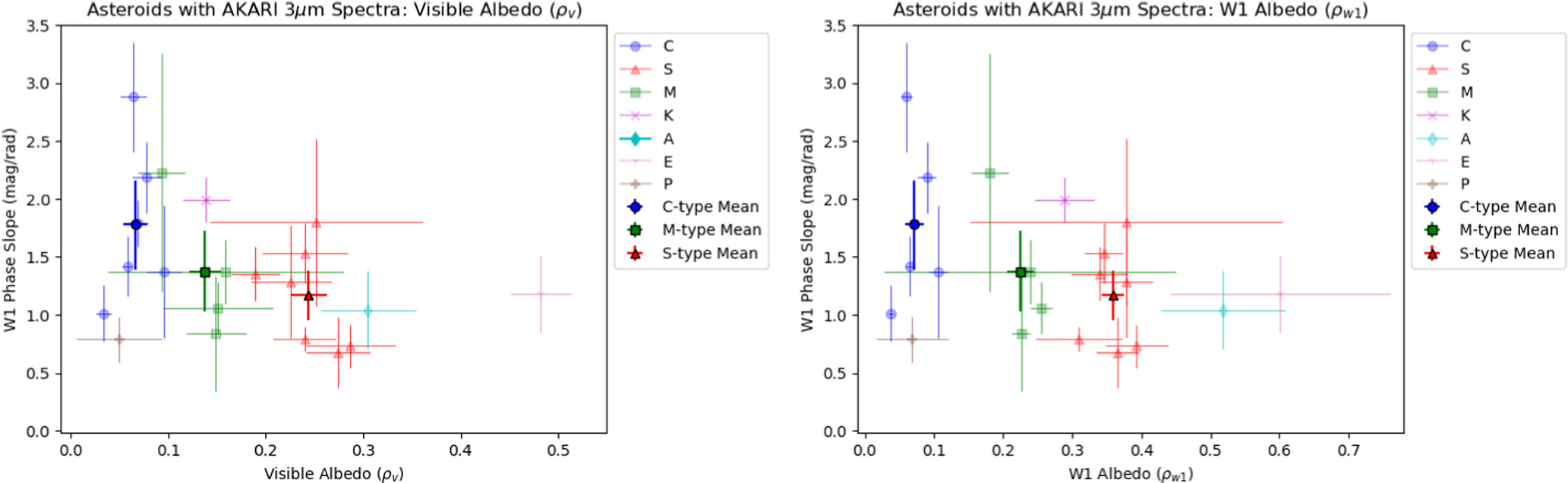
Figure 5. Left: W1 phase slopes of asteroids with 3 μm spectra from the AKARI mission vs. their visible albedo. Right: W1 phase slopes of asteroids with 3 μm spectra from the AKARI mission vs. their W1 albedo. The colors and shapes of the points correspond to the Tholen spectral classification of that asteroid. The bold points represent the mean phase slope vs. the mean albedo of the C, M, and S spectral types within our sample.
Download figure:
Standard image High-resolution imageFigure 6 shows the W1 phase slope versus the 3 μm spectral slope as measured by Usui et al. (2019). We see a lack of correlation when comparing the W1 phase slope to the spectral slope, although the spectral slope within the bandpass should also have an effect on the observed phase slope. Usui et al. (2019) measured their spectral slopes beginning at 2.6 μm and ending at a truncated wavelength value determined individually for each asteroid. The minimum truncated wavelength among all objects in our sample is 3.33 μm, while most objects have their spectral slope measured to beyond 3.5 μm, decidedly within the W1 bandpass. However, members of the C, M, and S classes all exhibit a range of spectral slopes and W1 phase slopes.
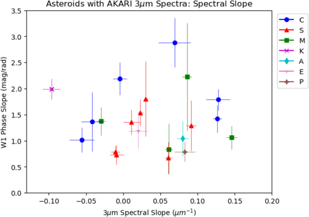
Figure 6. W1 phase slopes of asteroids with 3 μm spectra from the AKARI mission vs. their 3 μm spectral slope. The colors and shapes of the points correspond to the Tholen spectral classification of that asteroid.
Download figure:
Standard image High-resolution imageFigure 7 shows the same 21 asteroids but versus their 2.7 μm band depth (left) and 3.1 μm band depth (right). Interestingly, among C-type asteroids, there seems to be more of a trend in 2.7 μm band depth than in 3.1 μm band depth, despite the 2.7 μm falling just outside the W1 bandpass. The C-type asteroids had the deepest and most well-defined 2.7 μm features in the AKARI study, so it is encouraging to see the steepening of their phase slopes with increasing band depths given this band's association with hydrated materials.
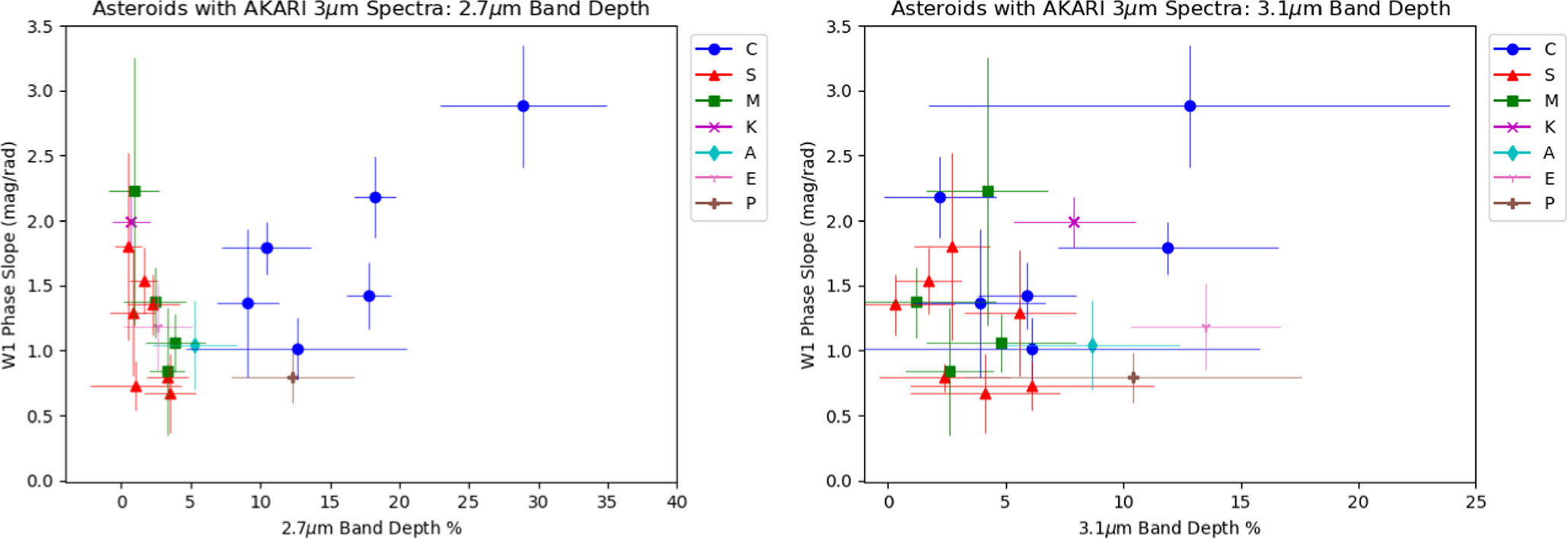
Figure 7. Left: W1 phase slopes of asteroids with 3 μm spectra from the AKARI mission vs. their 2.7 μm band depth as measured by Usui et al. (2019). Right: W1 phase slopes of asteroids with 3 μm spectra from the AKARI mission vs. their 3.1 μm band depth as measured by Usui et al. (2019). The colors and shapes of the points correspond to the Tholen spectral classification of that asteroid.
Download figure:
Standard image High-resolution image4.2. Themis Family
We present our results for the Themis family in two different scenarios, showing results before and after the S/N cutoff mentioned in Section 2 and included in Table 1. To help illustrate the motivation for the S/N cutoff, we also include results for the Flora family, an S-type family, for comparison. Precut, we measured phase slopes for 93 Themis-family asteroids, removing 11 asteroids from the sample due to the statistical constraints discussed in Section 3.3. We also remove six additional asteroids from the sample due to uncharacteristically high W1 albedos. Since C-complex asteroids (the dominant taxonomic type within the Themis family) are dark objects with low reflectivity, asteroids with high W1 albedos are potential interlopers that may not be true Themis family members. Masiero et al. (2014) computed the average W1 albedo of 95 Themis-family objects to be 0.073 ± 0.009 while also finding that main-belt asteroids separated into distinct groupings of 6%, 16%, and 40% W1 reflectivity. Based on these results, we impose a W1 albedo cutoff of 0.15, omitting any objects with higher W1 albedos. The six objects in our Themis sample with W1 albedos >0.15 were (2228) Soyuz-Apollo (1977 OH), (2587) Gardner (1980 OH), (3128) Obruchev (1979 FJ2), (5138) Gyoda (1990 VD2), (7314) Pevsner (2146 T-1), and (13649) (1996 PM4), none of which have identified taxonomic types. The W1 phase slopes for the remaining 76 Themis-family asteroids are shown in Figure 8, along with the W1 phase slopes for 91 Flora-family asteroids and 21 AKARI asteroids.
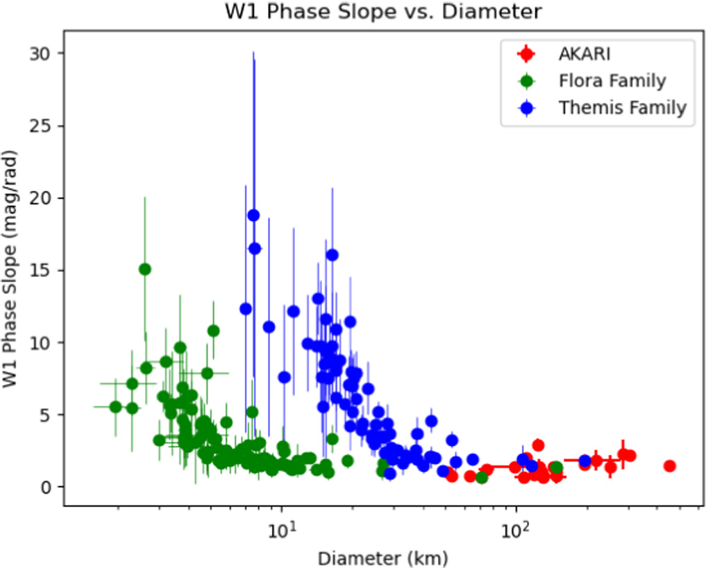
Figure 8. W1 phase slope vs. diameter (km) for Themis-family objects, Flora-family objects, and AKARI objects.
Download figure:
Standard image High-resolution imageThe smaller-diameter objects for both families show extremely steep phase slopes that would suggest highly abnormal phase curve shapes. However, the shift in diameter space between the Themis and Flora families implies that this is an observational effect rather than a physical effect. The differing semimajor axes of the two families (2.2 au for Flora and 3.13 au for Themis) likely play a role in the size at which the increase in phase slope happens, since small, high-albedo objects closer to the observer would be more easily detectable and have higher S/N than small, dark objects that are further away. To investigate this further, we looked at the phase angle coverage for each individual asteroid and the average S/N of the NEOWISE observations used to derive each point on the phase curve of an asteroid. These results are shown in Figures 9, 10, and 11. Figures 9 and 10 demonstrate that the steepening of the phase slope we see in Figure 8 is not merely a result of a decrease in phase angle coverage. This check was necessary to ensure that the same level of noise in the NEOWISE observations was not having a larger impact due to low phase coverage, thus affecting the relationship we observe between phase slope and diameter. Given the scatter shown in both plots, it is unlikely that a decrease in phase coverage is significantly impacting the observed trends in Figure 8, as there is no discernible change in W1 phase slope or diameter as the phase angle coverage decreases for either family. The phase angle range is determined using the minimum and maximum phase angle observed for each object, which is given in Table 3.
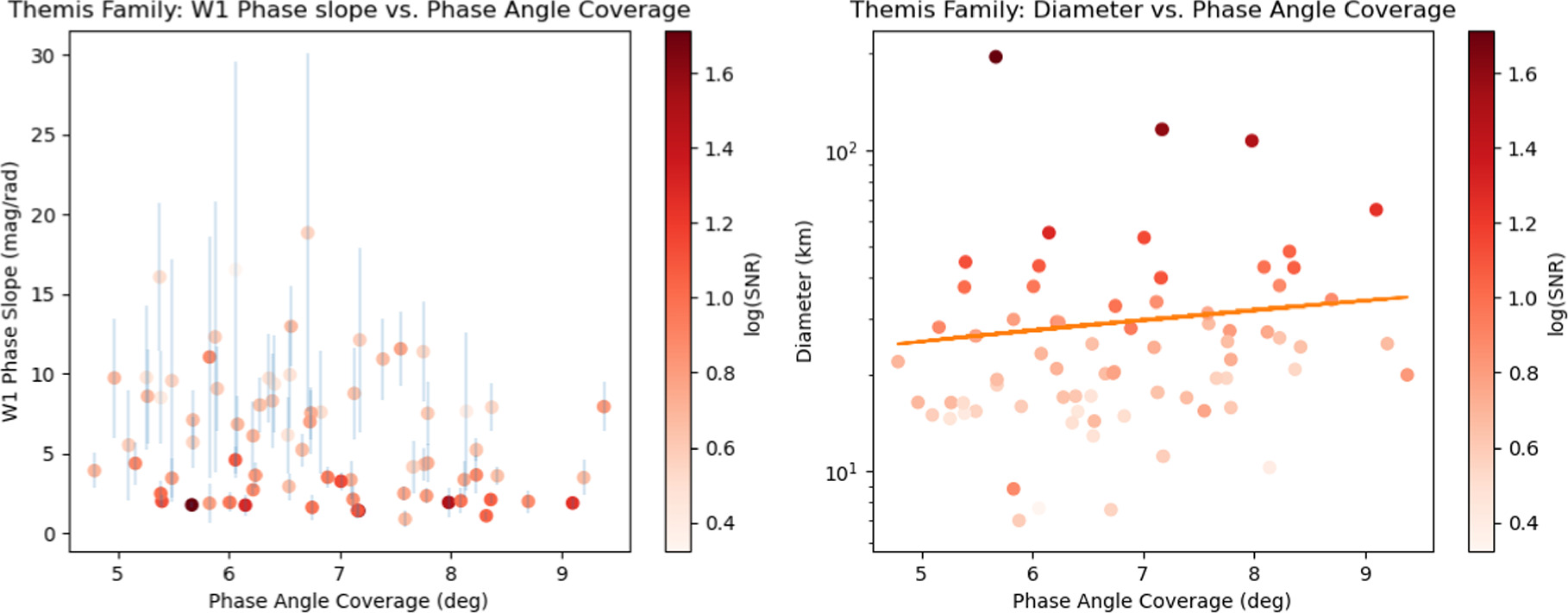
Figure 9. Left: W1 phase slope vs. phase angle coverage for Themis-family objects. Right: diameter vs. phase angle coverage for Themis-family objects. The orange line is a linear fit to the data.
Download figure:
Standard image High-resolution image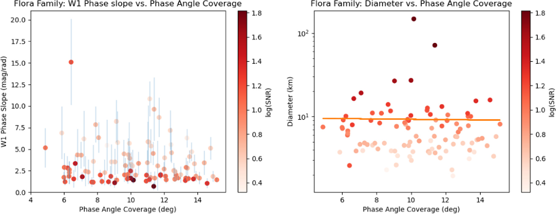
Figure 10. Left: W1 phase slope vs. phase angle coverage for Flora-family objects. Right: diameter vs. phase angle coverage for Flora-family objects. The orange line is a linear fit to the data.
Download figure:
Standard image High-resolution imageWe also investigated the S/N of the observations used to construct our W1 phase curves, shown in Figure 11. Here, we see that smaller-diameter objects with steeper phase slopes also have the lowest S/N observations, with an inflection point occurring around S/N = 7. It is likely that the smaller objects are having their lower-phase-angle magnitudes scattered upward due to a combination of detector noise and the Eddington bias, thus increasing the slope of their phase curves. This assertion is supported by the lack of low-S/N objects with small phase slopes and high-S/N objects with steep phase slopes. This was the motivating factor in excluding all NEOWISE observations with S/N < 7 and repeating our analysis. Moving forward, all results shown will be based on this updated analysis, from which any NEOWISE observations with S/N < 7 were excluded. Figure 12 is the updated version of Figure 8, and many of the steeper phase slopes have been eliminated (note the change in scaling for the y-axis). After imposing this S/N cutoff, the Themis sample contained 41 objects, and the Flora sample contained 64 objects.
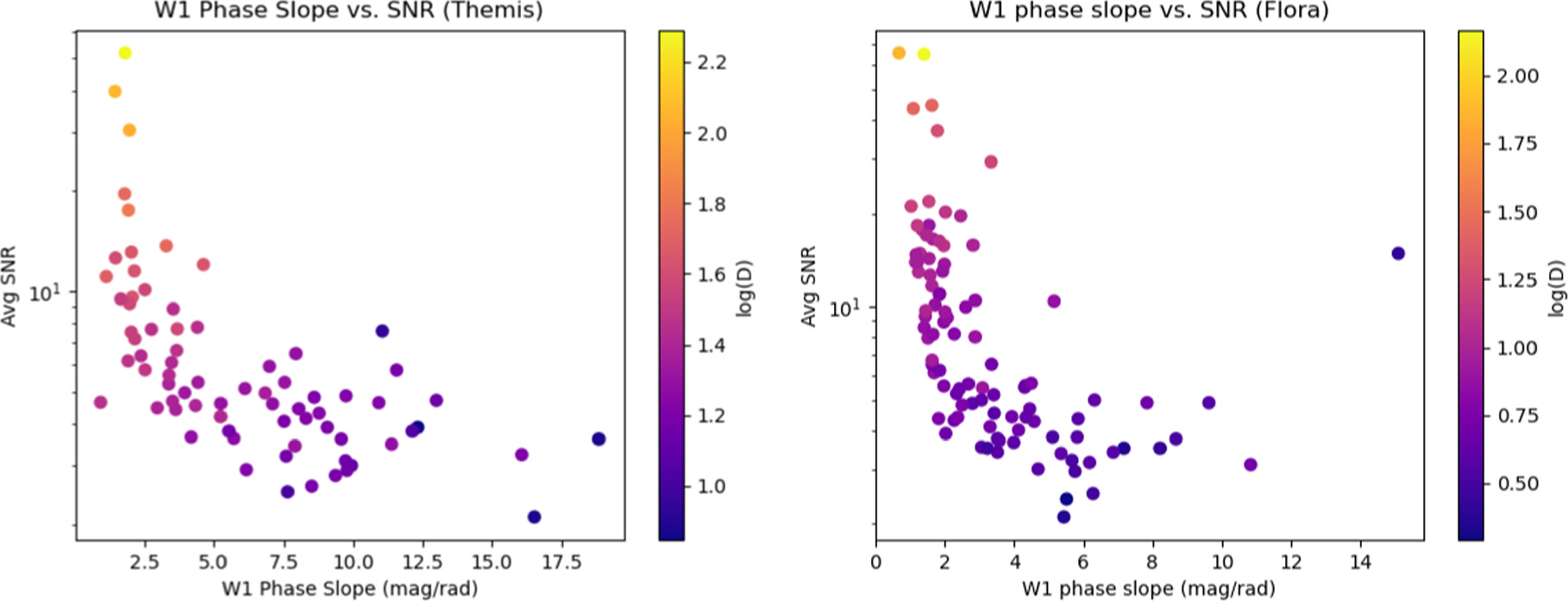
Figure 11. Average S/N vs. W1 phase slope for the Themis family (left) and the Flora family (right), colored by diameter. The S/Ns shown here are the average of the W1 observations used to determine the phase curve point for the lowest available phase angle for a given object.
Download figure:
Standard image High-resolution image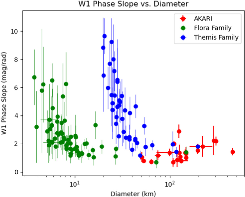
Figure 12. W1 phase slope vs. diameter (km) for Themis-family objects, Flora-family objects, and AKARI objects after removing all NEOWISE observations with S/N ≤ 7.
Download figure:
Standard image High-resolution imageFigure 13 shows the W1 phase slope of Themis-family objects versus the log of their W1 albedo. We see that the W1 albedos of the Themis sample objects tend to remain similar (as expected for C-types) despite changes in the size and phase slope of the object. This comparison was motivated by the results from Figure 25 in Kokotanekova et al. (2018), which showed an increase in phase slope versus R-band geometric albedo for JFCs despite decreases in phase slope as a function of albedo for both main-belt and near-Earth asteroids. Given that JFCs are expected to be volatile-rich, this is an intriguing comparison for the Themis family, which has several members with detected near-surface water ice and outgassing (Hsieh et al. 2004, 2010; Rivkin & Emery 2010; Hsieh et al. 2011). We saw a similar trend in the Themis sample before imposing the S/N cutoff, but post-cutoff, this trend is not apparent despite a few outliers at steep phase slopes and higher W1 albedos. It should also be noted that there are potential selection effects that could be impacting our sample. In order to measure a significant enough amount of reflected flux in W1, higher-albedo objects will be preferentially selected from an otherwise random sample. Smaller, low-albedo objects will have smaller fluxes at W1, increasing the likelihood that those objects would be absent from our sample due to lack of detection or reasonable phase coverage. Thus, these potential selection effects should be kept in mind during the discussion of our results.
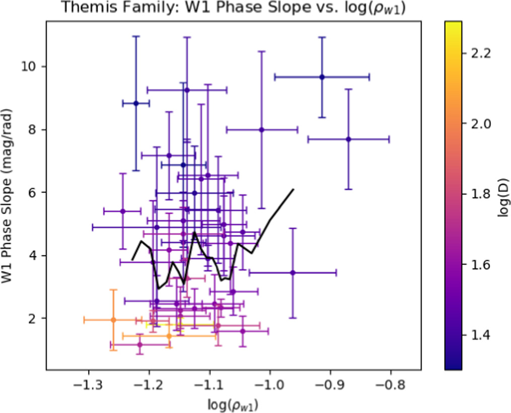
Figure 13. W1 phase slopes of Themis-family asteroids vs. their log W1 albedo. The black line represents a five-point running mean.
Download figure:
Standard image High-resolution image5. Discussion
Our intention in exploring the sample of AKARI asteroids was to search for any correlation between their W1 phase slope and their spectral properties indicative of the presence of hydrated materials or organics. We also included comparisons to their albedos to increase the scope of our results. When evaluating Figures 5–7, it can be useful to focus on the C, M, and S spectral types, as they represent low-, moderate-, and high-albedo populations, respectively. The expected breakout in albedo space is apparent, and there does appear to be a slight difference in the W1 phase slopes of C-, M- or S-type asteroids. Based on visible-light phase curves shown in Muinonen et al. (2002), we would expect lower-albedo asteroids (C-types) to exhibit steeper phase curves than higher-albedo M- or S-type asteroids. The mean phase slope versus albedo points shown for the C-, M-, and S-type objects in Figure 5 do loosely support this expectation, but given the error bars, a larger sample size is likely needed to more definitively determine if this trend holds in 3 μm light. However, the C-type objects in the AKARI sample do, on average, have steeper phase slopes than the M-types, which have slightly steeper phase slopes than the S-types, providing some support that our derived phase curves are reasonable.
Despite these results, there are factors we could not account for that may be impacting our phase curves in this sample. Buratti et al. (2022) constructed phase curves at multiple wavelengths for several of the icy moons of Saturn, noting that the slope of the linear portion of their phase curves decreased as the albedo of the object increased. However, they also noted a change in the shape of the opposition surge for these moons in their 3.60 μm phase curves. While our work does not cover phase angles that contribute to the opposition effect, Buratti et al. (2022) asserted that the observed difference in the 3.60 μm opposition effect could likely be attributed to the lack of interaction between these longer-wavelength photons with smaller particles on the object surface. Since the AKARI sample consists of mostly larger-diameter objects, which should have significant populations of small particles on their surfaces (Gundlach & Blum 2013), it is possible that minimal interaction between the surface regolith and light at 3 μm is having an effect on the observed phase slopes in the linear regime as well. At visible wavelengths, the opposition effect is thought to be caused by coherent backscattering and shadow hiding regardless of roughness, whereas at linear phase angles, brightness is more influenced by shadow hiding and single-particle scattering (Muinonen et al. 2002). Thus, surface roughness and particle size distribution could be playing a major role in affecting our derived phase slopes.
The left panel of Figure 7 shows a potential correlation between the 2.7 μm band depth and the W1 phase slope within the C-complex, despite a lack of any such correlation with the 3.1 μm band depth. Usui et al. (2019) determined that most C-type asteroids had clear absorption features in the 3 μm region, while most S-types had no significant features in this region. If these absorption features impact the phase curve at these wavelengths, then the comparison of W1 phase slopes between C- and S-type asteroids could be a reasonable method by which to make broad determinations about the presence of such features (and thus the presence of hydrated substances), provided they are significant enough. As seen in Figure 7, the increase in phase slope for C-types as a function of 2.7 μm band depth becomes most apparent at band depths above ∼15%. This may also explain why it is difficult to draw any conclusions from the 3.1 μm band depth sample, as the measured band depths there do not exceed 15%. Additionally, there are several asteroids of other spectral types that have similarly higher phase slopes despite having little to no measured 2.7 μm band depth. If we extrapolate from the visible regime, the higher-albedo objects should have flatter phase slopes, so it is notable that some objects associated with higher-albedo spectral types show steeper phase slopes similar to those of the low-albedo C-types with large absorption features. Both of these comparisons would benefit from a larger sample size, especially within the C-complex, which is expected to harbor more hydrated materials.
Being a family composed primarily of C-complex asteroids, the Themis family is a potential reservoir of hydrated materials. This is partially why the increase in C-type phase slope with 2.7 μm band depth is encouraging; however, comparisons between the Themis sample and the AKARI sample are difficult to make. Band depth measurements are not available for most Themis-family objects, so ideally, the AKARI sample would have served as a baseline with which to make determinations about the Themis sample based on their phase slopes. Despite the increase in W1 phase slope for AKARI C-types as a function of the 2.7 μm band depth, a comparison of the two samples in Figure 12 further illustrates that the phase slope is impacted by multiple factors, observational or physical, that can have a much larger impact on the phase slope than a significant absorption band. Since the AKARI sample lacks objects at smaller diameters, it is difficult to make any determinations about Themis-family objects based solely on the AKARI sample results. Additionally, there are likely observational selection effects impacting our sample, as there will be inherent biases in favor of detecting high-albedo objects. This should be taken into account when interpreting our results, as it is likely that (1) our sample does not adequately represent the population of small, low-albedo asteroids, and (2) the effects of detector noise combined with the Eddington bias are likely acting to steepen the derived slopes for smaller objects.
Despite these caveats and the difference in the diameters of our two samples, which may preclude us from using the AKARI sample to draw conclusions about hydrated materials in the Themis family, it still reveals a compelling trend in that smaller objects in the Themis family exhibit steeper phase slopes, as shown in Figure 12. We also included the AKARI sample in this comparison to illustrate that the W1 phase slope remains flat at larger diameters, suggesting that this may be a more global trend rather than one specific to the Themis family. While the S/N-based issues may still be impacting our derived phase slopes even after the S/N ≤ 7 cutoff, we offer the following possible physical interpretation for the observed trend with diameter, as well as reasoning that the steeper phase slopes may still be plausible.
According to Gundlach & Blum (2013), objects with diameters of less than ∼20 km are generally covered by relatively coarse regolith grains, with typical particle sizes in the millimeter-to-centimeter range, while larger objects with diameters bigger than ∼80 km have very small regolith particles with grain sizes between 10 and 100 μm. One possible explanation is that objects with a larger surface gravity are able to hold on to the finer, smaller particles more easily, as opposed to smaller objects that would only be able to gravitationally retain larger grains after an impact (Gundlach & Blum 2013). The uptick in phase slope we have here seems to begin around 30–40 km for the Themis family and around 10 km for the Flora family. Smaller particle sizes tend to result in higher overall reflectivity (Capaccioni et al. 1990), but it is unclear how this might relate directly to the phase slope. In the linear phase curve regime, the dominant mechanisms are shadow hiding and single-particle scattering, effects that are more pronounced for dark surfaces (e.g., C-type asteroids; Muinonen et al. 2002). Larger objects retain finer regolith, and small particle sizes mean better packing and smoother surfaces. These surface properties lead to less shadow hiding and more uniform scattering from single particles, which could explain the flatter phase curves we see at larger diameters. Other mechanisms that could contribute to particle size differences between large and small objects are space weathering (Clark et al. 2002; Anand et al. 2004; Nesvornỳ et al 2005) and thermal fatigue (Delbo et al. 2014). Statistically speaking, smaller asteroids tend to be younger than larger asteroids within the same family. For example, the Themis family is an old family (∼2.5 Gyr) that has likely experienced multiple disruption events (Nesvornỳ et al 2003; Leliwa-Kopystyński et al. 2009). Smaller objects resulting from later disruption events would have younger surfaces than older, larger objects in the sense that they have experienced less space weathering and thermal fatigue, both of which are processes that would cause the breakdown of surface particles into finer grains.
While the phase slopes for smaller-diameter objects in the Themis sample are quite steep, we note the large error bars for these slopes and compare to the distribution of linear phase slopes from Gaia observations shown in Table 3 and Figure 2 of Martikainen et al. (2021). Specifically, we compare to the  phase slopes, as these are brightness maxima–based phase slopes, similar to those shown in this work. While there are likely inherent differences between visible light and 3 μm light phase curves, it is notable that the tail end of the
  distribution approaches 5 mag rad–1. This suggests that our derived phase slopes are reasonable, even when considering the steepest slopes in our sample and their associated errors.
This physical interpretation does not, however, explain the difference in phase slope uptick diameter between the Flora and Themis families, which are S- and C-type families, respectively. S-type objects have higher W1 albedos than C-type objects and are thus expected to have flatter phase slopes, but our Flora sample also covers a smaller-diameter regime than our Themis sample. Larger surface particle sizes associated with smaller objects would act to steepen the phase slope, but the higher albedo of S-types would act to flatten the phase slope, so there may be some degeneracy between these factors. Despite this, more work on the exact relationship between grain size and the phase slope is needed at 3 μm wavelengths in order to explore this relationship further. This could be achieved through laboratory work, similar to Capaccioni et al. (1990), who performed visible reflectance measurements as a function of phase angle for several naturally occurring materials, or Kaasalainen et al. (2002), who made measurements at small phase angles for sand and meteorite rocks and made comparisons with the observed phase curve of asteroid (69) Hesperia. A Hapke model could also be implemented to more thoroughly explore how the grain size is expected to impact phase curves at these wavelengths (Hapke 1981, 1984, 1986, 1990, 2008, 2012). If the modeling indicates that smaller grain sizes would yield flatter phase curves at 3 μm region wavelengths, then this could lend support to our physical interpretation of the phase slope increases we see with respect to diameter in Figure 12.
For added context, we also investigate the W1 albedo as a function of diameter for the Themis-family asteroids and the C-types from the AKARI sample. We only include AKARI C-types because of the dependence of albedo on spectral type, as the other spectral types at large diameters have much higher albedos than the Themis-family asteroids. Since smaller objects within the Themis family show steeper phase slopes, we would expect these objects to have lower albedos based on what we know in the visible regime. This is not the case, however, as the smaller-diameter objects also show higher W1 albedos, on average. We use the diameter ranges given by Gundlach & Blum (2013) for context, although there is only one Themis-family object shown in Figure 12 below 20 km. The 37 asteroids between 20 and 80 km had an average W1 albedo of 0.079, while the nine asteroids >100 km had an average albedo of 0.069, suggesting a reverse trend in phase slope versus albedo space.
We further explore this reverse trend by directly comparing the W1 phase slope and W1 albedo within the Themis family in Figure 13. As mentioned in Section 4.2, we see that the W1 albedos of Themis objects remain clustered around ∼0.07 (∼−1.1 in log space), in spite of changes in the size and phase slope of the object. The motivation for this comparison was to investigate if Themis objects showed an increase in W1 phase slope with increasing W1 albedo, the opposite of what we would expect. Such a trend would draw some similarities to findings from Kokotanekova et al. (2018), who observed an increase in R-band phase slope with increasing R-band geometric albedo for JFCs. They hypothesized that the possible correlation they observed between the phase slope and R-band geometric albedo is representative of the evolution of JFCs over time. "Young" JFCs with high volatile content begin with relatively high albedos and steeper phase slopes. As they become more active, sublimation-driven activity makes their surfaces smoother and causes flatter phase slopes. Meanwhile, the nucleus becomes more covered in dust as the comet becomes less active and the sublimation gradually decreases. Coupled with the loss of volatiles, this causes the observed decrease in albedo as the phase slope also decreases. Following this hypothesis relating to the evolutionary track of JFCs, it is possible that Themis-family asteroids (or, more broadly, C-complex asteroids) experience a similar evolution in the sense that some of these objects once contained larger reservoirs of volatile material, and some may still harbor such material in the present day. However, we do not observe any strong correlation between the W1 phase slope and W1 albedo of our Themis sample objects, as most objects remain at typical C-type albedos despite an increasing phase slope. There are a small number of outliers at steeper phase slopes and above-average albedos, but a larger sample size of objects with high-S/N observations is needed to further explore this comparison to JFCs.
In summary, we find no discernible relationship between W1 phase slope and 3 μm spectral slope or 3 μm band depth for the sample of asteroids with available AKARI spectra. However, we do find distinct differences in the W1 phase slopes of C-, M-, and S-type objects in the AKARI sample, with the W1 phase slope going from steepest among C-types to flatter among M-types and flattest among S-types. This aligns with the expected behavior of the phase slope for these spectral types at visible wavelengths as well, based on their albedos. We also find that C-type asteroids with 2.7 μm absorption features above 15% in band depth may exhibit steeper phase slopes, but a larger sample is needed to determine a stronger correlation.
Objects within the C-complex Themis family show a distinct increase in W1 phase slope as their diameters decrease, even after the removal of low-S/N observations. This implies that there are inherent differences in the physical properties of the surfaces of smaller and larger objects. We suggest that the surface properties associated with larger (smaller particle sizes and smoother surfaces) and darker (more pronounced shadow hiding and single-particle scattering) objects lead to more uniform scattering and result in the observed flatter phase slopes for larger objects.
We search for trends between W1 phase slope, W1 albedo, and diameter within the Themis family that bear similarities to those shown by JFCs. Some JFCs show a reverse trend in R-band phase slope, where the phase slope steepens as the albedo increases and the diameter decreases. This comparison between the Themis family and JFCs would offer support to the idea that the Themis family may have once been (or may still be) volatile-rich. However, we do not find such a trend in Themis-family asteroids, although a larger sample size would assist in investigating this comparison further.
Acknowledgments
This publication makes use of data products from the Wide-field Infrared Survey Explorer, which is a joint project of the University of California, Los Angeles, and the Jet Propulsion Laboratory/California Institute of Technology, funded by the National Aeronautics and Space Administration. This publication also makes use of data products from NEOWISE, which is a project of the Jet Propulsion Laboratory/California Institute of Technology, funded by the Planetary Science Division of the National Aeronautics and Space Administration. This work was supported by the New Mexico Space Grant Consortium, a member of the congressionally funded National Space Grant College and Fellowship Program that has been administered by the National Aeronautics and Space Administration. Thank you to Przemysaw Bartczak for his work updating the ISAM database for this project. D.O. was supported by National Science Center, Poland, grant No. 2022/45/B/ST9/00267.
Appendix
This appendix contains Figure 14, a figure set comprised of all derived W1 phase curves for the asteroids in our sample.
Figure 14.
Data points are color coded by NEOWISE mission phase to indicate the origin of the observations used to derive a given point in the phase curve. Blue is NEOWISE reactivation, red is WISE two-band, green is WISE three-band (not pictured above for (5) Astraea), and black is WISE four-band. The orange line represents the least-squares linear regression best-fit line. The complete figure set (124 images) is available in the online journal. (The complete figure set (124 images) is available.)
Download figure:
Standard image High-resolution imageFootnotes
- 4
- 5