


Abstract
GRB 160821A is the third most energetic gamma-ray burst observed by the Fermi gamma-ray space telescope. Based on the observations made by the Cadmium Zinc Telluride Imager on board AstroSat, here we report the most conclusive evidence to date of (i) high linear polarization ( detection), and (ii) variation of polarization angle with time, occurring twice during the rise and decay phase of the burst at 3.5σ and 3.1σ detections, respectively. All confidence levels are reported for two parameters of interest. These observations strongly suggest synchrotron radiation produced in magnetic field lines that are highly ordered on angular scales of 1/Γ, where Γ is the Lorentz factor of the outflow.
Export citation and abstract BibTeX RIS
1. Introduction
Gamma-ray bursts (GRBs) are the most intense astrophysical outbursts in the universe. In the last several decades, the spectra of prompt gamma-ray emission of GRBs have been extensively studied using various space observatories such as the Burst and Transient Source Experiment (BATSE) on board the Compton Gamma-Ray Observatory (CGRO; Fishman 2013), Niel Gehrels Swift (Gehrels & Swift 2004), Fermi (Atwood et al. 2009; Meegan et al. 2009), etc. The radiation process producing the prompt gamma-ray emission, however, still remains a mystery. Polarization along with spectrum measurements can provide an insight into this long-standing enigma. Performing polarization measurements of prompt emission is highly challenging, mainly because of the scarcity of incident photons and the brevity of the event. Previously, polarization measurements of prompt gamma-ray emission were attempted only for a few cases by the Reuven Ramaty High Energy Solar Spectroscopic Imager (RHESSI; Coburn & Boggs 2003; Wigger et al. 2004), the INTErnational Gamma-Ray Astrophysics Laboratory (INTEGRAL; Götz et al. 2009, 2013, 2014; McGlynn et al. 2009), the GAmma-ray burst Polarimeter (GAP; Yonetoku et al. 2011, 2012), the Cadmium Zinc Telluride Imager (CZTI; Rao et al. 2016; Chattopadhyay et al. 2017; Chand et al. 2018, 2019), POLAR (Burgess et al. 2019; Zhang et al. 2019), etc. but the results were statistically less significant and sometimes unconvincing (for a recent review please refer to McConnell 2017). In this Letter, for the first time, we present conclusive evidence of polarization across the GRB 160821A in the energy range 100–300 keV using the CZTI instrument on board AstroSat (Singh et al. 2014).
On 2016 August 21, the Burst Alert Telescope (BAT) on board the Neil Gehrels Swift observatory (Gehrels & Swift 2004) triggered and located the GRB 160821A at (R.A., decl.) =(171.248, 42.343) with 3' uncertainty (Markwardt et al. 2016) at 20:34:30 UT, along with other space observatories such as Konus-Wind and the Gamma-Ray Burst monitor on board the CALorimetric Electron Telescope (CALET). However, due to solar observing constraints Swift could not slew to the BAT position until a week later. Hence, there were no X-ray or ultraviolet (UV)/optical telescope observations for this burst. Half an hour after the trigger time, an optical transient was detected by ground-based telescopes, but no redshift measurements could be made.
The Fermi Gamma-Ray Burst Monitor (GBM; Meegan et al.2009) also triggered on the burst at 20:34:30.04 UT (Stanbro & Meegan 2016). The GBM light curve included a precursor emission starting from trigger time, T0 until T0+112 s, followed by a bright emission episode with a duration T9011
of 43 s. For the time interval T0-4.1 s–T0+194.6 s, an energy flux of 2.86 ±0.007 × 10⁻⁶ erg cm−2 s−1 is obtained in 10–1000 keV band. This makes the burst the third brightest GRB observed by Fermi to date in terms of energy flux. The Fermi-Large Area Telescope (LAT; Atwood et al. 2009) detected emission in the LAT Low Energy (LLE) data (30–100 MeV), starting at T0+116 s and emission above 100 MeV starting at T0+130 s (Arimoto et al. 2016), with LAT emission extending up to ∼2000 s beyond the duration of GBM emission. AstroSat-CZTI also detected the burst for a duration T90 of 42 s (Bhalerao et al. 2016) and captured only the main episode of the burst. GRB 160821A was incident on CZTI from the direction, θ = 156 2 and ϕ = 592, thus coming through the side veto detector. Polarization measurement was attempted in the energy range 100–300 keV using ∼2549 detected Compton events (Chattopadhyay et al. 2014, 2017). In Figure 1(a), a composite 1 s binned light curve obtained from various detectors on board Fermi, AstroSat, and Swift satellites are shown. The present work focuses only on the results of the study of the main episode of the burst observed by both Fermi and AstroSat.
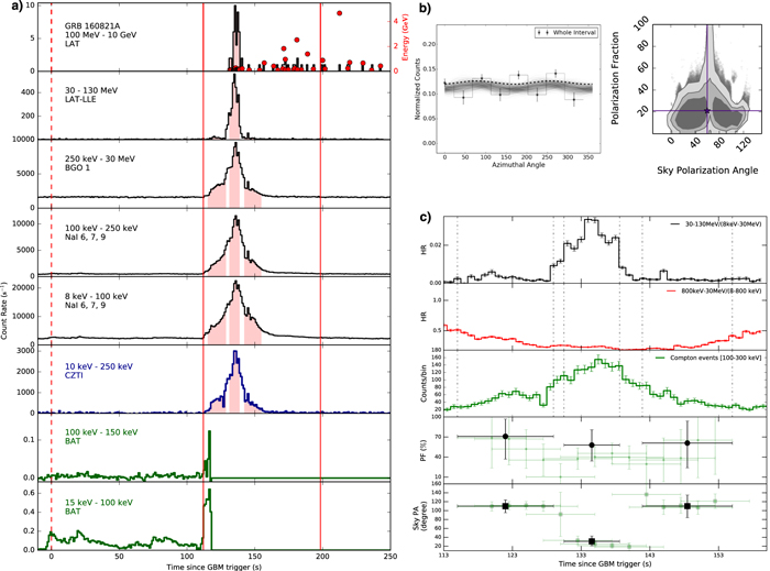
Figure 1. Panel (a): a composite 1 s binned light curve of the burst is shown for Fermi detectors: LAT, LAT-LLE, bismuth gallium oxide (BGO), sodium iodide (NaI), AstroSat/CZTI and Swift/BAT. The vertical dashed red line (at T0 = 0 s) corresponds to the trigger time of Fermi and the solid vertical red lines mark the beginning and end of the main episode of the burst. The Fermi/LAT photons whose probability of association with the same GRB is greater than 90% are shown as red points in the top right of the left panel with energy information scaling on the right side of y-axis. The time intervals studied in polarization analysis are shown in red shaded regions. Panels (b): left panel: the azimuthal distribution of Compton events and the best-fit modulation (dashed line) obtained for the entire main episode of the burst are shown. Modulation fits obtained for 1000 runs out of the 1.1 × 10⁷ simulation data sets are shown in the black shaded regions. Right panel: the 2D histogram plot of the obtained polarization fraction (PF) and polarization angle (PA) values along with the contours corresponding to confidence levels of 68%, 90%, and 99% are shown in darker to lighter black regions, which are overplotted on the scatter plot of PF and PA. The average values of PF and PA are marked by a violet star. Panel (c): the uppermost and second from the top sections show the hardness ratio (HR) of the counts LLE to sum of the counts in NaI 6 and BGO 1 (black), and ratio of the counts in BGO 1 to that of NaI 6 respectively. In the third section from the top, the 1 s binned CZTI Compton events (green) light curve is shown. The time intervals (black vertical dash dot lines) for which the temporal polarization study is done, are shown. The fourth and fifth sections from the top show the PF (black circles) and corresponding PA (black squares) obtained for these time intervals. Also, PF and PA values obtained in the fine time-resolved analysis are shown in the background in shaded green circles and squares, respectively.
Download figure:
Standard image High-resolution image2. Polarization Analysis
The measurement of polarization is obtained from the azimuthal distribution of Compton-scattered photons, which lie preferentially in a direction orthogonal to the incident electric field vector (Covino & Gotz 2016; McConnell 2017). The azimuthal distribution is fitted with the cosine function of the form

where ϕ0 is the polarization angle (PA) of the incident photons as measured in the CZTI detector plane, A/B is the modulation factor (μ), and η is the azimuthal angle (see also Zhang et al. 2019). The measured detector plane PA is converted into the celestial/sky reference frame by taking into account the satellite orientation at the time of observation, and these values are reported throughout the Letter unless otherwise mentioned. The polarization fraction (PF) is calculated by normalizing the modulation with μ100 (the modulation factor obtained for 100% polarized emission coming from the same direction of the GRB with the same spectrum) for the respective detector PA.
A low polarization ( ) was found at 90% (2.2σ) confidence level for two parameters of interest, when the entire pulse constituting a time interval of 115–155 s was analyzed (Figure 1(b)). All the errors quoted for polarization measurements in this Letter are at a 68% confidence interval for two parameters of interest including the systematic errors (Appendix A), unless otherwise mentioned. We find this result to be in agreement with the recent polarization observations of GRBs made by POLAR (Zhang et al. 2019), where they find the time-integrated emission of GRBs to possess a low PF. They suspect that such low polarization could be due to a change in PA within the pulses/across different pulses.
The evolution of the light curves observed by Fermi in different energy bands were characterized by studying the ratio of photon counts observed in high and low energies, parameterized as the hardness ratio (HR); see the uppermost and second from the top sections in Figure 1(c). We found that the emission above 30 MeV changed distinctly with respect to the rest of the burst after T0+129 s and T0+140 s. In addition to this, a fine time-resolved polarization analysis of the main episode was conducted. PF and PA for successive 10 s intervals shifted by 2.5 s were measured, thereby studying the evolutionary trend in PF and PA (Figure 1(c)). Such a methodology including overlapping time intervals was adopted because of the limited number of photons available in the smaller time intervals. Therefore, during the analysis we tried to constrain the PF such that at least the lower limit of 68% confidence interval of one parameter of interest was greater than zero. This is because if the time interval is unpolarized i.e., PF is consistent with zero, then its PA has no physical meaning. A change in PA was observed to occur twice as the burst transited from its rise to peak and later to its decay phases while PF was greater than zero.
We note that during the times when the PA angle makes a change, a decrease in PF is expected. Thus, based on the clear change in PA where we could constrain the polarization at a higher significance (i.e., the lower limit of a 99% confidence interval of two parameters of interest of PF are greater than zero) and the observed change in HR at high energies, we performed a relatively coarser time-resolved polarization analysis of the GRB by dividing the main episode into three non-overlapping time intervals: 115–129 s, 131–139 s, and 142–155 s, which correspond to the rise, peak, and decay phase of the burst, respectively.
2.1. Results
During the first time interval, the burst emission has a PF of  and a PA of
  . In the second interval, a
  with a corresponding
  and in the third interval, a
  with a corresponding
  , are determined (Figure 1(c)). By performing Monte Carlo simulations (Appendix B) of the data set of each interval, the posterior distributions of PF and PA of these intervals were also obtained. Intervals 1, 2, and 3 were found to be polarized at confidence levels of 99.8% (3.5σ), 99.97% (4σ), and 99.1% (3.1σ), respectively, for two parameters of interest (Figure 2). As the burst transits from its rise to the peak phase and then into its decay phase, the PA shifts by
  and
and  , respectively, (Figure 1(c)). The statistical significance of the change in PAs, Δ PA1, and Δ PA2 are determined at 3.5σ and 3.1σ, respectively, which are the minimum of the obtained statistical significance of the two intervals to be polarized. Other cases of varying polarization that were reported earlier are GRB 041219A (Götz et al. 2009), GRB 100826A (Yonetoku et al. 2011), and GRB 170114A (Zhang et al. 2019) observed by INTEGRAL, GAP, and POLAR, respectively. Consequently, the low PF found across the burst can now be understood as an artifact of the temporal change of PA occurring within the burst. The results of the polarization analysis of the three time intervals are listed in Table 1.
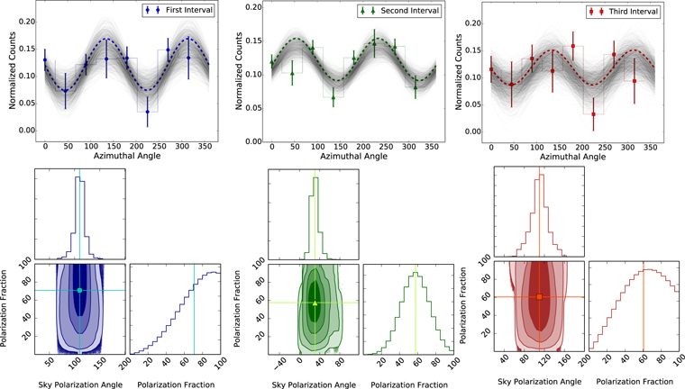
Figure 2. Top-left corner: for the first interval, the best-fit modulation curve obtained is shown in dashed blue line. Modulation fits obtained for 1000 out of  simulated data sets are shown here in shaded black. In the bottom-left corner, the 2D histogram plot of the obtained PF and PA values, along with the contours corresponding to confidence levels of 68%, 90%, 99%, and 99.9%, are shown in terms of darker to lighter shades of blue, which are overplotted on the scatter plot of PF and PA. Similar corresponding plots for interval 2 are shown in the top-middle and bottom-middle panels (green). For this time interval, an additional contour of confidence level 99.99% is shown in the 2D histogram plot. For interval 3, corresponding plots are shown in the top-right corner and bottom-right corner (red). The average values of PF and PA obtained in intervals 1, 2, and 3 are marked by the blue circle, green triangle, and red square, respectively, on their 2D histograms; they are also marked by solid lines on their respective posterior distribution plots.
Download figure:
Standard image High-resolution imageTable 1. Results of the Temporal Polarization Analysis
| Time Intervals (s) | 115–129 | 131–139 | 142–155 |
|---|---|---|---|
| Compton events | 896 | 1124 | 523 |
| Background events (s−1) | 20.7 ± 4.5 | 20.7 ± 4.5 | 20.7 ± 4.5 |
| MDP (99% confidence) | 40% | 32% | 57% |
| μa | 0.289 | 0.250 | 0.243 |
| μ100 | 0.409 | 0.435 | 0.403 |
| PFa |

|

|

|
| PAa |

|

|

|
| Confidence level | 99.8% | 99.97% | 99.1% |
Note.
aThe average values of μ, PF and PA from the posterior distribution are reported.Download table as: ASCIITypeset image
In order to estimate the average PF across the burst, (i) the first and the third intervals were combined because they had nearly same PAs (fourth section from the top of Figure 1(c)); and (ii) Monte Carlo simulations involving combined fits of this new interval and the second interval with the cosine function were performed. The PF related parameters A and B of the cosine functions were linked across the intervals, while the PAs were kept free. Thus, we found the average PF and the PAs for the new interval and the second interval. In Figure 3, the posterior distributions of the average PF across the burst and the corresponding change in PA estimated by taking the difference of the PAs of the new interval and interval 2 are shown. The average PF across the burst is estimated to be  at
at  confidence for two parameters of interest as shown in Figure 3. Also, we note that the change in PA estimate (
 ) is consistent with the average of the change in PAs that were found occurring within the burst. Previously, such a statistically significant polarization was reported for the burst GRB 021206 by Coburn & Boggs (2003); however, the claim was contested by the analyses performed by Rutledge & Fox (2004) and, subsequently, Wigger et al. (2004). Recently, POLAR found that the time-integrated emission of five bright GRBs possess the most probable PF, between 4% and 11% at a confidence level of 99.9% (Zhang et al. 2019). To date no other polarization measurement of GRBs reported by BATSE, INTEGRAL, GAP, AstroSat, or POLAR have obtained a statistical significance greater than ∼99.9% (Covino & Gotz 2016; McConnell 2017; Zhang et al. 2019).

Figure 3. 2D histogram plot of the average PF and the correspondingly obtained average change in polarization angle across the burst. Contours corresponding to confidence levels 68%, 90%, 99.7%, 99.99%, 99.99992% (5.3σ), and 99.99995% (5.4σ) are shown. The average values of PF and change in PA are marked on their respective posterior distributions by a solid black line.
Download figure:
Standard image High-resolution image3. Spectral Analysis
Traditionally, the GRB prompt emission spectrum is modeled using the phenomenological Band function12 (Band et al. 1993). The time-resolved spectral analysis of the main episode of the burst, however, shows significant deviations from the pure Band function in the brightest bins (Preece et al. 2014; Vianello et al. 2018). The deviation in lower energies is modeled by adding a blackbody (BB) function at kT ∼ 30 keV and, at higher energies by adding a cutoff at Ec ∼ 2–50 MeV (Appendix C). Thus, the spectrum is best modeled using a BB + Band × Highecut (Figure 4(a)), where the BB can be related to the thermal emission (a relic of the dense fireball that formed at the central engine after the explosion), and the rest to the non-thermal emission coming from the optically thin region of the outflow (Guiriec et al. 2011; Axelsson et al. 2012; Iyyani et al. 2013, 2016; Burgess et al. 2014; Vianello et al. 2018). The evolution of the spectral-fit parameters are shown in Figure 4(b). We note that the low-energy part of the spectrum characterized by the low-energy power-law index, α and the spectral peak, Ep are nearly steady throughout at ∼−0.97 and 800 keV, respectively. However, the high-energy part of the spectrum characterized by the high-energy power-law index β and cutoff Ec vary significantly such that β decreases, whereas Ec increases with time. After T0+140 s, these trends are reversed. This spectral behavior is consistent with the trend observed in HR reported above.
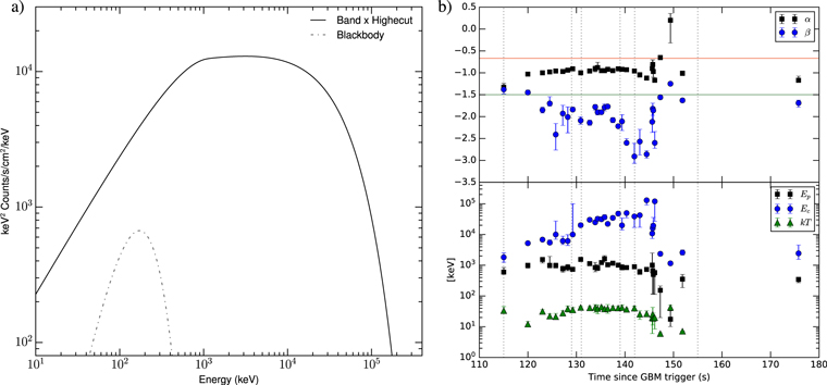
Figure 4. Panel (a): the  plot of the best-fit model, Band × Highecut (solid black line) + blackbody (BB; dashed−dotted black line), fitted to the brightest time interval, i.e., 134.59–135.71 s. Panel (b): the upper section shows the time evolution of α (black squares) and β (blue circles) of the Band function. The green and red horizontal lines in the upper section mark the photon index of α = −1.5 and α = −0.67, corresponding to the fast and slow cooling synchrotron emissions, respectively. In the lower section, the time evolution of the Band Ep (black squares), the high-energy cutoff Ec (blue circles), and the temperature of the BB component kT (green triangles) are shown. The three time intervals of polarization study are shown in dotted vertical black lines across the two panels.
Download figure:
Standard image High-resolution image4. Discussion and Summary
GRBs with long durations, >2 s, are associated with the death of massive stars. A highly collimated outflow (jet) of opening angle  , moving at a relativistic speed (parameterized by Lorentz factor,13
Γ) is produced after the core of the massive star collapses to a black hole (or a magnetar) and begins to accrete the surrounding stellar matter. The radiation emitted from this relativistic outflow is beamed toward the observer within a cone of 1/Γ, which is the visible region around the line of sight. This is referred to as the relativistic aberration/beaming.
, moving at a relativistic speed (parameterized by Lorentz factor,13
Γ) is produced after the core of the massive star collapses to a black hole (or a magnetar) and begins to accrete the surrounding stellar matter. The radiation emitted from this relativistic outflow is beamed toward the observer within a cone of 1/Γ, which is the visible region around the line of sight. This is referred to as the relativistic aberration/beaming.
In a classical fireball model (Mészáros 2006; Pe'er 2015; Iyyani 2018), where the outflow is non-magnetized, the non-thermal emission is generally expected to be produced in shocks created in the optically thin region above the photosphere from where the thermal emission is expected. Energetic electrons produced in the shocks then cool by processes such as synchrotron emission in random magnetic fields generated in the shocks (Ghisellini & Lazzati 1999), or inverse Compton scattering (Lazzati et al. 2004), both being inherently locally axisymmetric around the outflow's velocity vector. For a fixed viewing angle,14
 , in an axially symmetric jet, the polarization vector integrated over the spatially unresolved emitting region should point either perpendicular to or in the plane containing the axis of the jet and the line of sight of the observer. Thus, the PA is expected to change by 90° when the width of the jet parameterized by
  changes. In such a case, when the orientation of the polarization vector becomes perpendicular to the observer plane, the PF is expected to be low (<10%; Ghisellini & Lazzati 1999; Granot 2003; Toma et al. 2009). However, here we observe that during the entire burst, the PF values are >15%. Thus, a change in width of the visible portion of the jet cannot account for the observed change in PA. Inherently axisymmetric emission models referred to above are ruled out.
The total radiative energy15
released in the prompt emission of GRB 160821A is estimated to be Eγ,iso = 6.9 × 1053 (3.6 × 1055) erg, for a redshift, z = 0.4 (2), if the radiation were isotropic. These are among the highest known values for long GRBs (Racusin et al. 2011). Such a high Eγ,iso suggests that the emission is strongly collimated, with the jet pointing toward the observer such that the line of sight lies within the jet cone or just outside the edge of the jet ( ). In the above scenario, the strong observed polarization can be explained only by synchrotron emission produced in magnetic fields that are highly ordered within the viewing cone of 1/Γ.
If we assume that the observed burst emission is a single emission episode, then it is difficult to explain, using any known physical model, the observed high polarization along with a change in PA. On the other hand, the burst emission consists of multiple emission episodes and, depending on the dominance of the synchrotron emissions coming from the different regions, a change in PA can happen with time (also see Lazzati & Begelman 2009).
Thus, for the first time conclusive evidence of high and varying linear polarization is detected in a GRB. The observations are extremely constraining and challenging within the framework of currently proposed physical models for GRBs. This motivates further research into the development of a physical scenario that can explain the observations self consistently.
We would like to thank Dr. Christoffer Lundman, Prof. Pawan Kumar, and Dr. Santosh Roy for enlightening discussions. This publication uses data from the AstroSat mission of the Indian Space Research Organisation (ISRO), archived at the Indian Space Science Data Centre (ISSDC). CZT-Imager is built by a consortium of institutes across India, including the Tata Institute of Fundamental Research (TIFR), Mumbai, the Vikram Sarabhai Space Centre, Thiruvananthapuram, ISRO Satellite Centre (ISAC), Bengaluru, Inter University Centre for Astronomy and Astrophysics, Pune, Physical Research Laboratory, Ahmedabad, Space Application Centre, Ahmedabad. This research has made use of Fermi data obtained through High Energy Astrophysics Science Archive Research Center Online Service, provided by the NASA/Goddard Space Flight Center. The Geant4 simulations for this paper were performed using the HPC resources at The Inter-University Centre for Astronomy and Astrophysics (IUCAA) and Physical Research Laboratory (PRL).
Appendix A: Systematic Error Estimate in Polarization Measurement
CZTI on board AstroSat is an X-ray spectroscopic instrument and is experimentally verified for polarization measurement capability in 100–400 keV energy range for on-axis sources (Vadawale et al. 2015). CZTI functions as a wide field monitor at energies >100 keV because the CZTI collimators and other supporting structures become largely transparent above this energy. This enables it to detect GRBs and measure their polarization. In order to calculate the modulation factor for off-axis sources, a mass model of AstroSat was developed in Geant4 (version 4.10.02.p02). There are several possible sources of systematic errors in the measurement of polarization (Chattopadhyay et al. 2017). Below we list these sources and the error estimates are quoted for the case of GRB 160821A:
(i) An uncertainty can be induced in the observed μ due to different photon propagation paths through the spacecraft structures. This uncertainty is estimated by conducting  Geant4 simulations of this burst with the same spectra and incident direction to produce the same number of observed Compton events. The uncertainty on μ is thus estimated to be ∼8%–16% according to the different number of Compton events. (ii) The selection of background is also expected to induce some systematic errors. This was investigated by taking both pre- and post-GRB background independently, as well as in combination, in order to determine the modulation amplitude. The uncertainty on μ due to this is found to be <1%. (iii) The effect of localization uncertainty is studied. GRB 160821A is localized at R.A. = 171.25 and decl. = +42.33 at ±3' accuracy (Markwardt et al. 2016). The contribution of localization uncertainty on the obtained modulation amplitude and PA is found to <1%. (iv) The uncertainty associated with the spectral model of the GRB is investigated by varying the power-law index within its estimated 1 sigma error and we find the associated uncertainty on the observed modulation amplitude to be <1%. (v) Another source of systematic error could be the unequal quantum efficiency of the CZTI pixels. The relative pixel efficiency across the CZTI plane is found to vary within ≤5%, which produces negligible false-modulation amplitude.
In the μ100 estimations, the statistical error is quite small as the simulations are done for a large number (108) of incoming photons. The systematic errors are those associated with the sources (iii) and (iv), while the uncertainty associated with source (i) is estimated to be ≤1%. The value of μ100 strongly depends on the fitted PA. The uncertainty associated with this in the estimation of PF is taken care of in the Monte Carlo process to obtain the posterior distribution of PF (described in Appendix B), where for each fitted PA, the corresponding μ100 is used.
All of these uncertainties are propagated into the reported values of the limits of the 68% confidence interval of two parameters of interest, namely the observed PF and angle.
Appendix B: Monte Carlo Method to Obtain Posterior Distributions of PF and PA
The polarization signature in the GRB is estimated through the non-uniform azimuthal distribution of GRB counts. We calculate the normalized counts for eight bins whose mid-values correspond to azimuthal angles: 0°, 45°, 90°, 135°, 180°, 225°, 270°, and 315°. These angles are estimated in an anti-clockwise direction when CZTI is viewed from top. The corrected modulation curves are fitted for large number of iterations (10 million) using the Monte Carlo method for estimating the modulation factor and PA as follows.
- (a)For each azimuthal angle (ηi), and its corresponding normalized counts (
 ) and error (yerr,i), we pick a random value (yran,i), from a normal distribution, which is defined by the mean value, and the standard deviation, . A normal distribution is assumed because, in the case of GRB 160821A, each azimuthal angular bin has over 20 Compton events (Cash 1979).
 - (b)The A, B, and ϕ0 parameters of the fitting cosine function given in Equation (1) are estimated for each set of randomly drawn yran,i (where i = 1–8) values via least square curve fitting method. For the fitted PA, the corresponding interpolated value of μ100, from a table of μ100 values that were generated for a discrete grid of PAs via the Geant4 simulations of 100% polarized emission for the same GRB spectra and incoming direction, is chosen. Thereby, estimating the PF values.
- (c)The above two steps are repeated for a large number of times (107), thereby obtaining the various required likelihood distributions of PF and PA.
- (d)The obtained likelihood is then filtered through the prior condition so that the PF has to lie between 0% and 100%. The simulation runs that satisfied the prior condition were then used to generate the posterior distribution.
- (e)Finally, the respective 2D histograms of posterior distributions of PA and PF are made.


Appendix C: Time-resolved Spectroscopy
For analysis of the Fermi GBM data, three NaI detectors with the highest count rates were chosen, namely n6, n7 and n9. These detectors observed the GRB at an off-axis angle less than 40°. In addition, the BGO detector BGO 1, which had the strongest detection, was chosen for analysis. LAT data (>100 MeV) belonging to the P8_TRANSIENT020E class and its corresponding instrument response were used, whereas the LAT-LLE spectra (30–130 MeV) were obtained using the same method as that for GBM data. The spectrum for each Fermi detector was extracted using the software Fermi Burst Analysis GUI v 02-01-00p1 (gtburst316 ). The background was obtained by fitting a polynomial function to the data regions before and after the GRB for time intervals, T0 − 410 s to T0 − 10 s and T0 + 210 s to T0 + 250 s, respectively.
A joint spectral analysis of Fermi GBM along with LAT-LLE and LAT data was carried out in Xspec (Arnaud 1996) 12.9.0n software and Pg-stat (Arnaud 2013) statistic was used. For NaI data, energies between 30 and 40 keV corresponding to iodine K-edge and extreme edges such as energies below 10 keV and above 850 keV were removed. In case of BGO, LAT-LLE, and LAT, data between energies 300 keV–10 MeV, 30 MeV–130 MeV, and 100 MeV–5 GeV were used, respectively.
For time-resolved spectroscopy of the burst, time intervals were defined using Bayesian Blocks algorithm on the detector (n6) with largest number of counts. In the tails of the emission episode, due to low signal-to-noise ratio, certain blocks were combined to get a larger time interval so that good spectral constraints could be obtained.
For estimating the effective area correction17
for NaI and LAT detectors, the bright time bins were simultaneously fitted with the best-fit model; i.e., BB + Band × Highecut multiplied with a constant of normalization, while the constant of normalization of the BGO 1 detector was fixed to unity. The relative normalization constants  for n6,
  for n7,
  , and for n9 and
  for LAT were obtained. Throughout the time-resolved spectral analysis, the effective area corrections for the detectors were frozen to these obtained values.
C.1. Statistical Significance Test
We conduct Monte Carlo simulations in order to ascertain the statistical significance of the deviations in the spectrum from a pure Band function, which have been modeled using a BB and cutoff at lower and higher energies, respectively (see the fit residuals in Figure 5). Because this process is computationally intensive, we present here the simulation study done for the brightest time bin (134.59–135.71 s) only, and adopt the obtained Δ Pg-stat distribution as a reference to assess the statistical significance of these components in other time bins.
- (a)BB: the difference in statistics, i.e., Δ Pg-stat, obtained for the model BB + Band × Highecut (fBHec) from fBHec is 24.5. We assume the model fBHec with the best-fit model parameters as the null hypothesis (H0) and generate nearly 40,000 realizations and its corresponding background spectra using the fakeit command in Xspec. Each of these realizations are then fit with the null hypothesis model fBHec and the alternate hypothesis (H1) model BB + fBHec, and the respective Δ Pg-stat values are recorded. The probability of observing any Δ Pg-stat of >24.5 is found to be 10−4.3 (Figure 6(a)), which corresponds to a significance level of ∼4σ.
- (b)Highecut: the Δ Pg-stat obtained for the model BB +fBHec from BB + Band is 201. In this case, we assume the model BB + Band with the best-fit model parameters as the H0 and generate nearly 54,000 realizations and its corresponding background spectra. The model BB + fBHec is the H1, and the respective complementary cumulative distribution of Δ Pg-stat is obtained. The probability to obtain Δ Pg-stat = 14 is (Figure 6(b)) which indicates that the probability to obtain any Δ Pg-stat > 201 is ≪10−4.5, which corresponds to a significance level of >4.2σ. Thus, the addition of Highecut to the Band function is highly significant.


Figure 5. Residuals obtained for the different models, Band, Band + BB, and BB +fBHec, fits done to the spectral data of the brightest time interval.
Download figure:
Standard image High-resolution image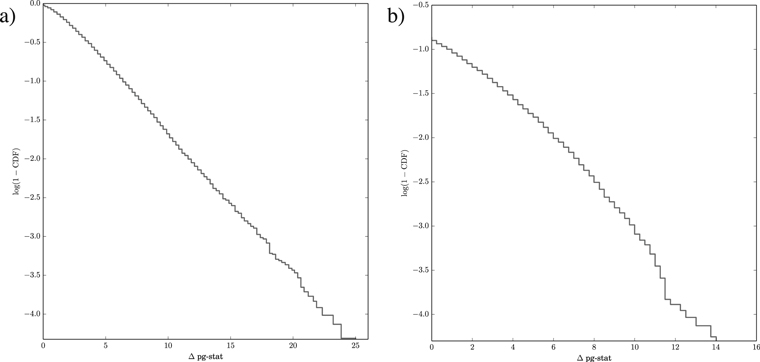
Figure 6. Complementary cumulative distribution function of the pg-stat obtained for models (a) fBHec function vs. BB + fBHec, and (b) BB + Band function vs. BB + fBHec are shown.
Download figure:
Standard image High-resolution imageFootnotes
- 11
T90 for Fermi (or AstroSat) is defined as the time duration between the epochs when 5% and 95% of the total photon counts of the burst are detected in the energy range 50–300 keV (40–200 keV).
- 12
Band function is an empirical function consisting of two power laws smoothly joined at a peak.
- 13 where v is the velocity of the outflow and c is the speed of light.
- 14 is the angle between the line of sight of the observer and the jet axis.
- 15
We find a fluence of
erg cm−2 in 10 keV–5 GeV. Fluence is the energy flux integrated over the duration of the burst. We assume a flat universe ( and km s−1 Mpc−1). - 16
- 17
An effective area of an instrument translates to its sensitivity, which can be different at different energies and off-axis angles from the axis of the instrument. In order to perform a combined spectral analysis of the data from different instruments such NaI, BGO, and LAT, a correction needs to be applied between these instruments, keeping one of them as the reference. This is estimated by multiplying a constant, independent of energy, with the normalization of the spectral model chosen for each instrument during the spectral analysis.


