


ABSTRACT
Modern observations revealed rich dynamics within solar prominences. The globally stable quiescent prominences, characterized by the presence of thin vertical threads and falling knobs, are frequently invaded by small rising dark plumes. These dynamic phenomena are related to magnetic Rayleigh–Taylor instability, since prominence matter, 100 times denser than surrounding coronal plasma, is lifted against gravity by weak magnetic field. To get a deeper understanding of the physics behind these phenomena, we use three-dimensional magnetohydrodynamic simulations to investigate the nonlinear magnetoconvective motions in a twin-layer prominence in a macroscopic model from chromospheric layers up to 30 Mm height. The properties of simulated falling "fingers" and uprising bubbles are consistent with those in observed vertical threads and rising plumes in quiescent prominences. Both sheets of the twin-layer prominence show a strongly coherent evolution due to their magnetic connectivity, and demonstrate collective kink deformation. Our model suggests that the vertical threads of the prominence as seen in an edge-on view, and the apparent horizontal threads of the filament when seen top-down are different appearances of the same structures. Synthetic images of the modeled twin-layer prominence reflect the strong degree of mixing established over the entire prominence structure, in agreement with the observations.
Export citation and abstract BibTeX RIS
1. RAYLEIGH–TAYLOR IN PROMINENCE STRUCTURES
Solar prominences are magnetized plasma about 100 times denser than their surrounding coronal plasma. Although supported by magnetic field against solar gravity, the dense plasma of prominences is susceptible to Rayleigh–Taylor (RT) instability, lying above lighter coronal plasma in a gravitationally stratified atmosphere. Quiescent prominences in the solar corona are globally stable, with typical lifetimes of weeks, but are locally very dynamic. With high-resolution observations using the Hinode Solar Optical Telescope, Berger et al. (2008) revealed that quiescent prominences are composed of bright vertical threads that are several hundred kilometers in width and host downflow streams with typical speeds of 10 km s−1 and lifetimes of about 10 minutes. Meanwhile, dark inclusions caused by upflows at 20 km s−1 rise from the base of the prominence up to 18 Mm heights, shedding voids on their way up. Further observations showed that the dark upflows preferably originate at the top edges of large-scale (20–50 Mm) arches that inflate from below into prominences, and they can grow from small perturbations to plumes of 4–6 Mm in widths that propagate 10–15 Mm in height (Berger et al. 2010). Measurements using the Atmospheric Imaging Assembly (AIA) instrument on board the Solar Dynamics Observatory (SDO) suggest that both the buoyant arches and these rising plumes contain plasma of 0.25–1.2 MK, 25–120 times hotter plasma than the prominence proper (Berger et al. 2011), suggesting a magnetothermal convection process occurring in the cavity-prominence system. While being bright above the solar limb, prominences appear as dark filaments against the bright solar disk. Filaments appear as a narrow spine above polarity inversion lines of photospheric magnetograms, and high-resolution observations revealed that filaments are composed of a collection of parallel thin threads, which are typically 2–20 Mm in length and 100–200 km in width making angles of 40°–90° with respect to filament spines (Lin et al. 2005). It is not clear whether the vertical threads of prominences are related to the apparent horizontal threads of the filament, due to a lack of high-resolution observations on a prominence from two distinct viewing angles at the same time.
Using a local model based on the Kippenhahn–Schlüter prominence model (Kippenhahn & Schlüter 1957), Hillier et al. (2012a, 2012b) performed three-dimensional (3D) magnetohydrodynamic (MHD) simulations on the RT instability mode development in the lower regions of a prominence structure. This demonstrated both plumes of upflows and descending plasma knots, resulting from interchange reconnection. 3D numerical global models of prominence dynamics in sheared magnetic arcade systems with effects of line-tying on the photosphere by Terradas et al. (2015) found that RT instability can be suppressed by low plasma β and large shearing angles of the supporting magnetic field. More recently, Terradas et al. (2016) studied the nonlinear evolution of dense prominences inserted in flux rope structures, where the near-alignment of the prominence axis and the magnetic field was found to suppress RT instability. In a 3D macroscopic prominence setup with dominating horizontal magnetic field, Keppens et al. (2015) included chromosphere–corona stratifications and simulated the RT phenomenon of the prominence well into the nonlinear magnetoconvective motions. They found upwelling pillars forming within rising bubbles and chromospheric material hurled up to very large heights. Since more complex structures like two adjacent filament branches are observed (see Figure 2 in Lin et al. 2005), we set up a twin-layer configuration and simulate the observed magnetothermal convective motions.
2. NUMERICAL SETUP
We use a Cartesian simulation box with an extension of 30 × 30 × 30 Mm, with gravity pointing along the negative y-direction. Using three levels of adaptive grid refinement we achieve an effective resolution of 600 × 600 × 600, with the smallest grid cell size of 50 km. We set the initial magnetic field B = (0.8, 0, Bz) Gauss to be planar and non-uniform with an exponential decrease (with height) of the strongest component Bz between a height y1 = 11.25 Mm (the bottom of the prominence) and a height y2 = 17.5 Mm. The analytic form of Bz is given by
where parameters are B0 = 8 G and λ = 15 Mm. The decaying magnetic field within the prominence's heights establishes an upward magnetic pressure force that lifts matter against solar gravity while inducing a continuous shear (up to 3°) of the planar field with respect to heights. To set up an equilibrium in the vertical direction including a chromosphere, the prominence, and a corona, we adopt a 7000 K temperature for the chromosphere, 1.8 MK for the corona, 6000 K for the lower part of the prominence, and a linear increasing profile of temperature from 6000 to 14,000 K for the upper part of the prominence. We use hyperbolic tangent functions to smoothly connect different temperature values in the stratified atmosphere. Then density and gas pressure are derived from the magnetohydrostatic equation assuming full ionization and an ideal gas law. The temperature and the density profiles along vertical line cuts through the prominence (solid line) and outside the prominence (dashed line) are plotted in Figures 1(b) and (c), respectively. The prominence is composed of two identical parallel layers, which have the same horizontal thickness of 5000 km and sandwich a 4000 km thick coronal region in between (see Figure 1(a)). Initially, the twin-layer prominence extends from a height of 11.25 to 20 Mm while being uniformly elongated in the x-direction. This initial setup represents the essential characteristics of solar prominences, as the density contrast at the bottom of the prominence is about 293. The total prominence mass in the computational box is about 1.9 × 10¹⁴ g. To add initial perturbations, we use a superposition of 50 small-amplitude sinusoidal velocity fields, periodic in the x-direction with random phases, localized at the bottom of each layer of the prominence. This phase randomness is also taken differently for each layer. We use periodic boundary conditions for the four side boundaries and fix all boundary values at the bottom. For the top boundary, the density and pressure are extrapolated from inner cells assuming hydrostatic equilibrium, the magnetic field is extrapolated assuming zero normal gradient, and the velocity field is copied from inner cells. With MPI-AMRVAC (Keppens et al. 2012; Porth et al. 2014), we numerically solve the ideal MHD equations using a Harten-Lax-van Leer Riemann solver (Davis 1988).
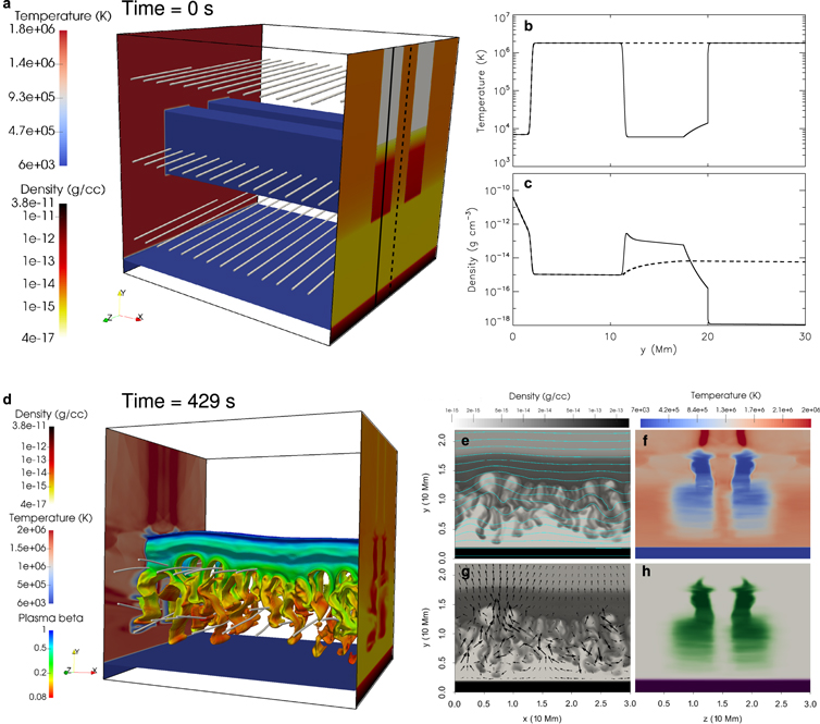
Figure 1. (a) A 3D view of a twin-layer prominence in the initial state with temperature contours showing the transition region and surfaces of the prominence, two vertical slices at the left and right sides presenting the temperature and density structures, and representative magnetic field lines. The temperature and the density profiles along the vertical line cut through the prominence (solid line) and outside the prominence (dashed line) are plotted in (b) and (c), respectively. (d) A 3D view of a snapshot at a time of 429 s, in which the tracing fluid contour (with the value of 0.95), colored by local plasma beta, showing the surfaces of prominence material with representative field lines. (e) and (g) show (z-)averaged density with projected magnetic field lines in light blue and black arrows sampling the integrated velocity field in the plane. The (x-)averaged temperature and tracing fluid are shown in (f) and (h), respectively.
Download figure:
Standard image High-resolution image3. TWIN-LAYER PROMINENCE DYNAMICS
To monitor the plasma in different regions, we use a tracing fluid that initially takes values of −1, 0, and 1, in the chromosphere, the corona, and the prominence, respectively. The tracing fluid is merely advected with the local velocity field. At any later time, we consider the chromosphere to have tracing fluid values less than −0.95, the corona between −0.05 and 0.05, and the prominence larger than 0.95. The integrated physical quantities of the prominence are plotted in Figure 2. Though being vertically force-balanced, the initial condition deviates from horizontal equilibrium in regions above y1, at the prominence–corona transitions because of gas pressure jumps there in the z-direction. The gradients of gas pressure generate shock waves in the corona above the prominence and the upper part (above 17.5 Mm) of the prominence, which traverse the periodic z-direction range in 85 s and are found to gradually damp out. Although the shocks lead to compression and heating of the prominence and the corona above, the essential characteristics, such as the total prominence mass and corona–prominence density and temperature contrasts, are maintained. Meanwhile, the RT stability is developing at the bottom of the prominence due to the seeded velocity perturbations. The shock-induced transverse motions quickly decrease and become dominated by RT vertical motions, as shown in Figure 2(a) where the kinetic energy evolution of the prominence is plotted for each velocity component. The vertical kinetic energy increases because of increasing vertical velocity induced by RT instability, until a time of about 480 s when the first falling RT fingers reach the relatively rigid floor—chromosphere and falling motions are restrained. We also quantify the prominence–internal energy balance in Figure 2(b). During the transient phase, the magnetic energy of the prominence drops by half mainly because the prominence is compressed along the magnetic field in response to the force imbalance. After the transient phase, the steady decrease of the gravitational potential energy of the prominence indicates falling prominence plasma, while the increase of magnetic energy is clearly in phase with the increase of the prominence volume, indicating that the expansion of the prominence is mainly along the magnetic field. The fluctuation of the overall increasing internal energy is out of phase with the fluctuation in volume, reflecting adiabatic compression and expansion of the prominence matter. The initially dominating potential energy becomes comparable with the magnetic energy at the end of our simulation. The total kinetic energy of the prominence is an order of magnitude smaller than all other kinds of energy. As RT instability develops, falling prominence plasma deforms the dominating horizontal magnetic field and the vertical component of magnetic field By increases and saturates at about 0.6 G, as plotted in Figure 2(c).
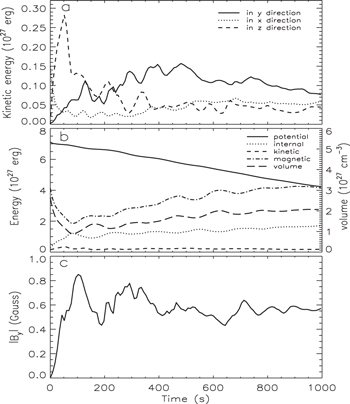
Figure 2. Time evolution of physical quantities of the prominence. (a) Kinetic energy in y (solid line), x (dotted line), and z (dashed line) directions. (b) Gravitational potential energy (solid line), internal energy (dotted line), kinetic energy (dashed line), magnetic energy (dashed–dotted line), and the volume of the prominence (long dashed line). (c) Mean magnitude of vertical magnetic component By.
Download figure:
Standard image High-resolution imageWe then focus on a snapshot at 429 s, when the longest falling RT finger is about to touch down the chromosphere. A 3D view of the data in Figure 1(d) clearly shows 3D RT fingers and bubbles by isosurfaces of the prominence, where the local plasma beta is smaller at lower altitudes mainly because of the stronger local magnetic field. Magnetic field lines of the upwelling bubbles are slightly bent concave-upward while field lines of the falling fingers are concave-downward, and these field lines are inter-changing without noticeable reconnection. Views from one side of the prominence shown in panels (e) and (g) of Figure 1 contain the z-averaged density, depicting falling RT dense pillars with typical width from 500 to 1000 km and rising light bubbles through the prominence body with lateral dimensions between 2000 and 5000 km. Although the front layer and the back layer of the prominence experienced different random initial perturbations, they develop similar RT patterns because they are connected and influenced by the same horizontal magnetic field lines. When viewing along the direction of magnetic field, the front and the back layer roughly overlap. When viewing along the z-direction, a small angle away from the direction of magnetic field, the overlap in RT structure on both layers appears shifted. As the magnetic field is frozen in the plasma, the initially horizontal magnetic field is deformed by vertical plasma motions, which is indicated in panel (e) by drawing streamlines of z-integrated in-plane magnetic field components Bx and By. The motions of upwelling coronal bubbles and falling prominence fingers are indicated by superposed arrows in panel (g) sampling the integrated velocity field. Looking from another viewing angle, along the prominence axis, Figures 1(f) and (h) provide views of temperature and tracing fluid, averaged along the x-direction, showing the twin-layer prominence fully embedded within coronal plasma, while the lower regions of the prominence that are disturbed by RT instability are extending vertically. The tracing fluid in panel (h) presents prominence matter in green, chromosphere plasma in dark purple, and coronal material in white. The narrower width in the upper part of the prominence resulting from the stronger compression there is caused by larger initial pressure differences at higher altitudes. This is consistent with the averaged temperature structures presented in panel (f), with blue indicating cool chromospheric and prominence matter, and red regions showing hot coronal plasma.
To compare the RT development in the each layer of the prominence, we make a vertical slice through each layer at z = ±3000 km with heights between 2600 and 15,000 km from the beginning until 429 s (see examples in the top and middle rows of Figure 3). At each time, we average tracing fluid values on these slices over the y-direction. This then provides a 1D quantification of typical structure along the x-direction in each layer. We then show the temporal evolution of their Fourier transform (in modulus and normalized by its maximum at each instant) as a function of wavenumber (reciprocal for wave length) in Figure 3. The random perturbations in velocity quickly translate to deformations up to wavenumbers of the order of 40, but after several tens of seconds, structure below wavenumber 20 (i.e., longer than 500 km) dominates. Especially pronounced structures show peaks at wavenumber ∼10 after 230 s, which translate to typical features of a size of 1000 km. The two layers of the prominence show similar-sized structures that dominate their evolution, but also noticeable differences in their instantaneous smaller-scale features.
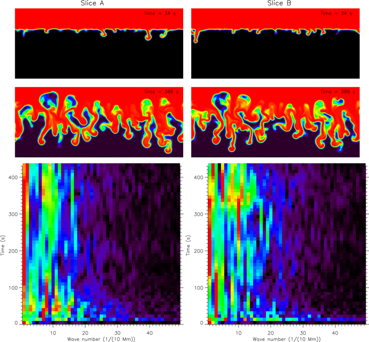
Figure 3. Two vertical slices colored by tracing fluid, through each layer of the prominence at 34 s (top row) and 386 s (middle row). Absolute values of Fourier transform of y-averaged structures in the slices are plotted in the bottom row.
Download figure:
Standard image High-resolution imageTo get views like observations on filaments, we integrate density and temperature from the top along the y-direction until reaching a height of 2500 km, excluding contributions from the transition region and chromosphere. These integrals are then divided by the length of the integration path to get mean values. The resulting 2D images at three selected moments are collected in Figure 4. The filament is composed of dense and thin threads that are roughly parallel to each other along local magnetic field lines with less dense gaps in between. The threads are typically 4–7 Mm in length and 150–300 km in width, which is consistent with observations. Comparing with flank views on the prominence in Figure 1(e), we find that each thread corresponds to a falling RT finger that naturally has a high column density in the vertical direction. In our model, the vertical threads of the prominence and the apparent horizontal threads of the filament are the same structures with different appearances due to different viewing angles. Besides, the dense threads are relatively cool, as we can see in the temperature maps where every dense thread corresponds to a low-temperature stripe that appears more dispersed. At a time of 429 s, the two filament spines of the twin-layer prominence are straight but fragmented into dark lumps and gray gaps that correspond to the rising hot RT bubbles. The structures in both layers evolve similarly because of their connection through the magnetic field. At a later time of 773 s, dark lumps of density in the left half of the filament disappear. That is because in the left half, large RT bubbles have filled most space and reached the top of the prominence, and the RT fingers have touched the chromosphere and become curved by the resulting turbulent flows that facilitate mixing of cool and hot plasma. Meanwhile, the average temperature of the filament decreases and develops more and larger low-temperature stripes. At the final time of 996 s, both layers of the filament become kinked in a very similar pattern. This kinking is induced by coherent lateral velocities in opposite directions at different locations of the filament, developed during the highly nonlinear evolution along magnetic field lines. The prominence thus shows a kind of collective kink deformation, with both layers clearly behaving as a single multi-layered large-scale entity. Apparently kinked filaments have been observed (see Figure 4 in Lin et al. 2005).
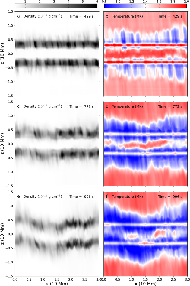
Figure 4. Top views of y-averaged density (left) and temperature (right), excluding regions with heights lower than 2500 km, at 429 s (top row), 773 s (middle row), and 996 s (bottom row). The grayscale density images are plotted in the left column with the temperature images in the right column.
Download figure:
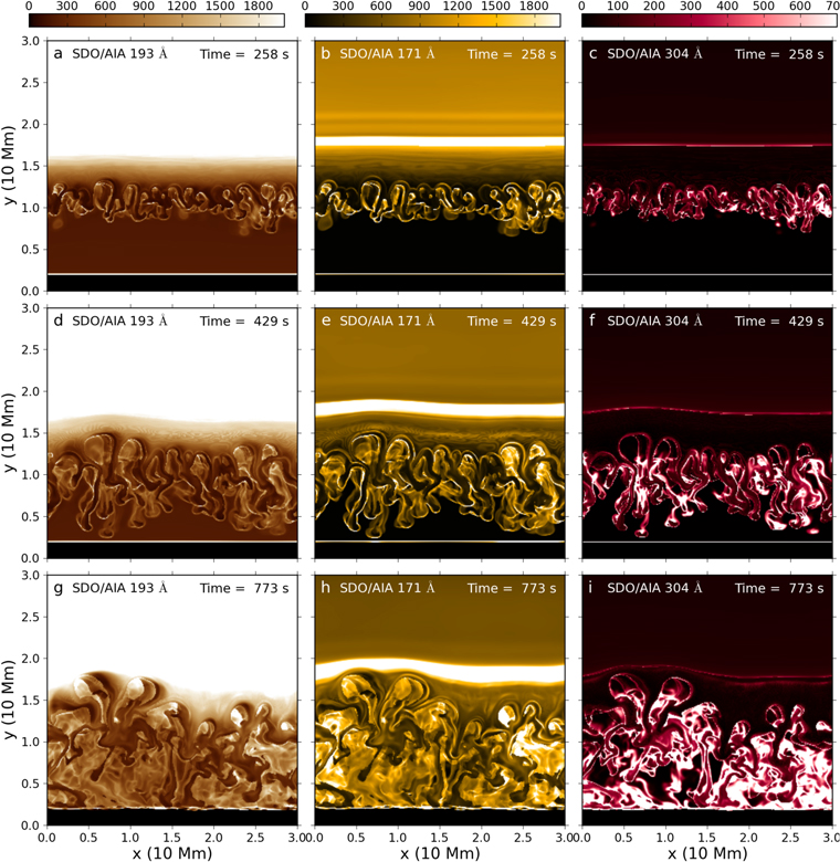
Standard image High-resolution imageUsing ray-tracing techniques, we can translate our 3D data into synthetic 2D images recorded in extreme ultraviolet (EUV), for direct comparison with those available from actual observations by AIA, which has 304, 171, and 193 Å channels highlighting matter at 80,000, 800,000 K, and 1,500,000 K, respectively. Synthetic EUV images in these channels with a line of sight along the lateral z-direction are collected in Figure 5, where the three rows are at three instants, i.e., 258, 429, and 773 s. Since we assume that material denser than 4.68 × 10⁻¹⁴ g cm−3 blocks any light from behind completely and less dense material is optically thin, the dense falling fingers have dark stems and bright edges in hot 171 and 193 Å channels, and they appear bright and thinner in the cool 304 Å channel. The RT fingers have cool cores embedded in hotter material with sheath layers due to the gradual to abrupt temperature and density transitions there, and they have leading ends shaped like mushroom caps. The rising bubbles are indeed composed of hot coronal material with bright emission in the 193 Å channel and no emission in the 304 Å channel. In the time sequence, we find that as the bubbles are rising with an average speed of about 15 km s−1, they inflate and squeeze their neighbors. Meanwhile, the falling fingers develop between bubbles and have an average descending speed of about 36 km s−1. The finger roots curve below their commensal bubbles, as they get squeezed together to close the bubbles. As the fingers are impacting the chromosphere, turbulent flows develop and whirl upward, perturbing all regions up to the top of the prominence. Bright emissions in the lower parts of 171 and 304 Å images at a time of 773 s (see Figures 5(h) and (i)) reflect warm plasma resulting from mixing of hot and cool plasma by these turbulent flows.
Figure 5. SDO AIA views along the z-direction at 258 s (top row), 429 s (middle row), and 773 s (bottom row), in channels of 193 Å (left column), 171 Å (middle column), and 304 Å (right column).
Download figure:
Standard image High-resolution image
4. CONCLUSIONS
We performed 3D MHD simulations on the internal dynamics of a twin-layer prominence starting in dominantly horizontal magnetic field and a vertically force-balanced gravitational stratified solar atmosphere. The properties of our simulated falling RT fingers and uprising bubbles are in line with those in observed vertical threads and rising plumes in quiescent prominences. The initial evolution of the two layers of the prominence is very similar as far as typical structure emergence and growth is concerned, due to their connection through the supporting magnetic field, which gets interchanged in the RT process. In the turbulent phase after RT fingers fall on to the chromosphere, the similarity decreases and the mixing of hot and cool material is very effective. Still, the twin-layer structure shows coherent large-scale kink deformations across the two layers. Our model suggests that the vertical threads of the prominence and the apparent horizontal threads of the filament are merely different appearances of the same structures from different viewing angles. Synthetic EUV images of the modeled prominence show remarkable agreement with observations. This pure ideal MHD model can be improved by considering more realistic magnetic configuration like using the Kippenhahn–Schlüter model (Hillier et al. 2012a) and by including important effects like thermal conduction, radiative cooling, coronal heating, and partial ionization. All these processes will make the actual temperature conditions even closer to observational findings, and are likely to influence and change, in particular, details beyond our current 50 km resolution. It is also left to future work how multi-layer large-scale prominences may form naturally, invoking, e.g., thermal instability routes (Keppens & Xia 2014; Xia et al. 2014; Xia & Keppens 2016) and then becoming subject to magnetothermal convection in realistic magnetic flux rope structures, where a strong magnetic field along prominences produces a stabilizing effect for RT instability (Terradas et al. 2016).
This research was supported by FWO (Research Foundation Flanders) and the Interuniversity Attraction Poles Programme by the Belgian Science Policy Office (IAP P7/08 CHARM). The simulations were conducted on the VSC (Flemish Supercomputer Center funded by Hercules foundation and Flemish government).