


Abstract
Most solar radio telescopes operate below ∼18 GHz and cannot realize a complete frequency coverage of the microwave spectrum, especially in the optically thin regime during solar bursts, which can provide unique information about the magnetic field in the burst area in the solar corona. Therefore, the development of high-frequency microwave observation equipment is demanded by the solar radio community. In this paper, we present a microwave spectrum observation system operating at 35–40 GHz. In this system, the solar radio signal is acquired by an 80 cm Cassegrain circularly polarized antenna, which is then downconverted and channelized by a 35–40 GHz analog front end. The processed signal is finally sent to the digital receiver to generate the microwave dynamic spectrum, which is transmitted by gigabit Ethernet transmission to a host computer. The system performance has been tested and obtained as follows: a noise figure of ∼300 K, system linearity of >0.9999, time resolution of about 134 ms (default), and frequency resolution of 153 kHz. We further conduct calibration for this system and find that the observed Sun–Moon ratio is about 43.1–53.3 @ 35.25 GHz during the new Moon, and is quite close to the theoretical value. The coefficient of variation of the system is ∼0.61% in a 9 hr test. The system has been designed, developed, and tested for over 1 yr in Chashan Solar Observatory and is expected to play an important role in the microwave burst study in the 25th solar cycle.
Export citation and abstract BibTeX RIS

Original content from this work may be used under the terms of the Creative Commons Attribution 4.0 licence. Any further distribution of this work must maintain attribution to the author(s) and the title of the work, journal citation and DOI.
1. Introduction
Solar eruptions, e.g., coronal mass ejections and flares, are generated by the release of coronal magnetic energy and can lead to severe space weather catastrophes in the solar–terrestrial space (Fletcher et al. 2011; Shibata & Magara 2011). Microwave bursts that can be observed by ground-based instruments are generally believed to be generated by the gyrosynchrotron emission process (Nakajima et al. 1985) and can be used to diagnose the magnetic field in the burst area of the solar corona. And, therefore, microwave observation could be an important option in the study of the triggering of solar eruptions.
So far, most solar-dedicated radio telescopes work below 18 GHz and cannot provide a complete frequency coverage of the solar microwave burst dynamic spectrum, especially in the optically thin regime. For example, the Humain Solar Radio Spectrometer (Marqué et al. 2018) provides a dynamic spectrum from 275–1495 MHz with a spectral resolution of 98 kHz and time resolution of 0.25 s. The multiwave Siberian Radioheliograph (SRH), which is upgraded by the Siberian Solar Radio Telescope (SSRT), will image the Sun at 3–24 GHz, and routine observation has first been carried out in five frequencies (4.5, 5.2, 6.0, 6.8, and 7.5 GHz) since 2016 (Lesovoi et al. 2017; Altyntsev et al. 2020). The Expanded Owens Valley Solar Array (EOVSA; Gary 2016; Gary et al. 2018) works in the frequency range of 1–18 GHz, and the Mingantu Ultrawide Spectral Radiohliogragh (MUSER; Yan et al. 2009; Wang et al. 2013; Liu et al. 2019) could cover the observations from 0.4–15 GHz. The Nobeyama Radioheliograph (NoRH; Nakajima et al. 1994), though working at 17 and 34 GHz, was closed on 2020 March 31. The Nobeyama Radio Polarimeters (NoRP; Nakajima et al. 1985), which once routinely observed solar microwave emission of up to 80 GHz, cannot provide data above 17 GHz. Some of the major solar radio instruments are listed in Table 1 (Smolkov et al. 1986; Mercier et al. 1988; Karlicky et al. 1998; Fu et al. 2004; Benz et al. 2009; Sawant et al. 2009; Carley et al. 2020).
Table 1. The Majority of Equipment for Solar Radio (>5 GHz)
| No. | Category | Name | Location | Available Year | Frequency (GHz) | Dedicated |
|---|---|---|---|---|---|---|
| 1 | Flux | MRO RT-1.8 | Finland | 1978 | 11.2 | No |
| 2 | Flux | SSRT | Russia | 1983 | 2–24, 4–8 | Yes |
| 3 | Flux | NoRP | Japan | 1984 | 1, 2, 3.75, 9.4, 17, 35, 80 | Yes |
| 4 | Flux | RT-32 | Latvia | 1998 | 6.3–9.3 | No |
| 5 | Flux | SST | Argentina | 1999 | 212, 405 | Yes |
| 6 | Spectrograph | SBRS | China | 2000 | 0.7–7.6 | Yes |
| 7 | Spectrograph | Ondrejov | Czech Rep. | 2009 | RT4: 2–5 | Yes |
| 8 | Spectrograph | Phoenix-3 | Switzerland | 2009 | 1–5 | Yes |
| 9 | Imaging | MRO RT-14 | Finland | 1978 | 37 | Yes |
| 10 | Imaging | NoRH | Japan | 1992 | 17, 34 | Yes |
| 11 | Imaging | RATAN-600 | Russia | 1997 | 0.7–18.2 | No |
| 12 | Imaging | MUSER | China | 2014 | 0.4–15 | Yes |
| 13 | Imaging | EOVSA | USA | 2015 | 1–18 | Yes |
| 14 | Imaging | SRH | Russia | 2016 | 3–24 | Yes |
Download table as: ASCIITypeset image
To develop a commonly used microwave observing system, we designed and manufactured a broadband radio telescope. This telescope has been tested to monitor solar radio observations in the frequency range of 35–40 GHz in Chashan Solar Observatory (CSO). In the working frequency range, the frequency resolution is 153 kHz, and the time cadence is about 134 ms with a default accumulation number of 1024. We will further extend the application of this system to acquire a full-coverage spectrum in the frequency range of 15–40 GHz. A two-element interferometer working at 39.5–40 GHz will be constructed to improve the systematic sensitivity. The next section presents the design of the observing system. Section 3 shows the tested performance of this system. Section 4 displays the data products. Section 5 describes the rough calibration of the data. The conclusion and discussion are given in the last section.
2. Receiver System
The developed broadband solar radio observing system is composed of a signal acquisition module, an analog front end (AFE), a digital receiver, and a host computer (the diagram shown in Figure 1 (a)). In this system (Figure 1 (b)), solar emissions acquired by a newly designed 80 cm dish (Yan et al. 2021) are divided into two channels and downconverted to an intermediate frequency (IF) of 937.5 ± 250 MHz by the AFE. The IF signal is then processed by a digital receiver (Yan et al. 2020) to generate the final dynamic spectrum. The basic performance parameters of this system are illustrated in Table 2.
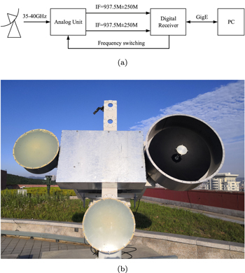
Figure 1. (a) The block diagram of the system. (b) The prototype of the system.
Download figure:
Standard image High-resolution imageTable 2. The Main Parameters of the 35–40 GHz Solar Radio Telescope
| No. | Parameter | Value |
|---|---|---|
| 1 | Frequency | 35–40 GHz |
| 2 | Antenna Gain | ∼45 dBi |
| 3 | Antenna Polarization | LCP |
| 4 | HPBW | ∼48' |
| 5 | Noise Figure | ∼300 K |
| 6 | Sampling Bandwidth | 1 GHz @ 2 channels |
| 7 | Sampling Rate | 1.25 GSPS |
| 8 | Resolution | 14 bit |
| 9 | Time Resolution | 134 ms (default) |
| 10 | Frequency Resolution | 153 kHz |
| 11 | System Linearity | >0.9999 |
| 12 | Coefficient of Variation | ∼0.61%/9 hr |
Download table as: ASCIITypeset image
2.1. The Antenna Unit
A Cassegrain antenna-feed system is designed to be the receiving unit of the observation system. The antenna is designed with left-hand circular polarization (LCP) to receive the one polarized component during the bursts. The primary reflector is developed with carbon fiber to reduce its weight, as a result of which the load of the track platform could also be reduced by a large extent. The diameter of the dish is designed to be 80 cm to improve the signal-to-noise ratio of the system. The half-power beamwidth (HPBW) of the main lobe is ∼0.8° in the frequency range of 35–40 GHz with a sidelobe suppression of >20 dB, and the gain of the antenna is about 45 dBi around 35.25 GHz (Figure 2). The feed is mounted just under the secondary reflective surface and acquires a solar radio signal after a two-step reflection. The HPBW of the feed is about 16° (Figure 2 (a)).
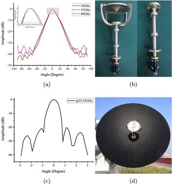
Figure 2. (a) The feed radiation patterns at 35 (black), 37 (red), and 40 (purple) GHz. (b) The prototype of feed with the secondary reflector. (c) The antenna radiation pattern at 35.25 GHz, the main lobe is ∼0.8°. (d) The prototype of the antenna-feed system.
Download figure:
Standard image High-resolution image2.2. The Analog Unit
The AFE lies behind the acquisition module. This module is used to process the analog signal received by the antenna-feed system to the working domain of the following digital receiver; the corresponding diagram is shown in Figure 3. The received signal is amplified, filtered, and downconverted to the IF of 937.5 ± 250 MHz. We note that a two-step downconversion is used to eliminate the deterioration resulting from intermodulation components with the first-level IF of 9 GHz ± 500 MHz and the second-level IF of 937.5 MHz ± 250 MHz. The filters follow the amplifier and mixer to suppress the image frequency and the intermodulation frequency, respectively.
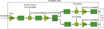
Figure 3. The design diagram of the AFE.
Download figure:
Standard image High-resolution image2.3. The Digital Receiver
The digital receiver converts the analog signal to a digital one, and processes these signals to the final dynamic spectrum. This receiver is composed of a motherboard and a daughterboard, and the two boards are connected via field-programmable gate array (FPGA) Mezzanine Card high-pin connector (Figure 4).
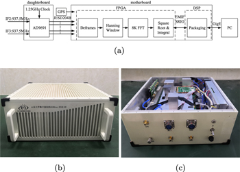
Figure 4. (a) The designed diagram of the digital receiver. The daughterboard transmitted the time-domain data to the FPGA on the motherboard by JESD204B. The motherboard completed the digital signal processing: deframing, the Hanning window, 8k-point fast Fourier transform (FFT), square root, and integration are finished in the FPGA, while packaging, timestamping, and uploading are accomplished in the digital signal processor (DSP). (b), (c) The prototype of the receiving system.
Download figure:
Standard image High-resolution imageIn this digital receiver, the IF analog signals from the AFE are first converted into digital ones by an analog-to-digital converter (ADC) on the daughterboard, and then transmitted to the motherboard by a serial protocol. We note that the ADC is the critical device for signal conversion, and it determines the performance of the digital part of the system. Therefore, AD9691 (14 bit 1.25 GSPS) is chosen, with the consideration of the demanded application in a wide frequency domain, and compatible with a wide frequency range (as shown in Figure 5). The input frequency range can be better adapted by selectively soldering resistors and capacitors of the different values given in Table 3 (Analog Devices 2015; Shi et al. 2020; Virkler et al. 2020).
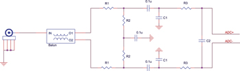
Figure 5. The input of ADC hardware design. The single-ended input is converted to a differential input by Balun to suppress common-mode interference.
Download figure:
Standard image High-resolution imageTable 3. The Values of the Component at the Different Frequencies
| Freq. (MHz) | R1 (Ω) | R2 (Ω) | R3 (Ω) | C1(pF) | C2(pF) |
|---|---|---|---|---|---|
| <625 | 10 | 50 | 15 | Open | 3 |
| >625 | 10 | 50 | 0 | Open | Open |
Download table as: ASCIITypeset image
The motherboard is compatible with the FPGA XC7K410T and the DSP TMS320C6678 completes the signal processing and transmits the data to the host computer. A series of signal processing tasks are finished in the FPGA, e.g., receiving data, deframing, and 8k-point FFT. The FPGA is configured with the same JESD204B protocol, the same number of lanes (eight), and at the same data rates (6.25 Gbps per lane) as the ADC to achieve handshaking. Data deframing is done by calling the FPGA intellectual property core to separate the data of the two ADCs from the JESD204B serial data. As illustrated in Figure 6, the base-2 time extraction butterfly operation is used to increase the speed of the operation (Yan et al. 2021). Packing, timestamping, and uploading are accomplished in the DSP.

Figure 6. The diagram of the 8k-point FFT algorithm for each channel of the ADCs (Channel A for example). Data in the time domain is divided into eight subgroups. Data in each group is then processed with a Hanning window and 1k-point FFT. The final three-step butterfly operation uses FPGA logic resources to accelerate the operation.
Download figure:
Standard image High-resolution image3. System Performance
The system has been tested to evaluate its performance. In the following, we present the performance of the system in terms of gain, noise figure, linearity, and stability.
3.1. The Gain and Noise Figure of the System
We know that the lower the noise figure, the higher the sensitivity of the system, so the noise figure should be reduced if possible. At the same time, a reasonable system gain will allow a suitable dynamic range for solar activities.
The system noise figure is determined by the amplifier cascade principle

where Fsys is the noise figure of the system, F1 (F2, F3) are the noise figures of the first-stage (second-stage, third-stage) amplifier contribution, respectively, and G1 (G2) is the gain of the first stage (second stage). As can be seen from Equation (1), the system noise figure is mainly determined by the first-stage amplifier, and the noise figure can be improved by choosing a first-stage device with a lower noise figure and large gain. In the developed system, we choose SBL-2734034025-KF as the first-stage low-noise amplifier (LNA), and the noise figure and gain are ∼300 K and ∼40 dB from 35–40 GHz at room temperature, respectively (see Figure 7).

Figure 7. (a) The first LNA noise figure. (b) The gain of the analog unit. Each 1 GHz bandwidth has a similar shape due to the effect of the filter, and the gain decreases with increasing frequency.
Download figure:
Standard image High-resolution imageReasonable design for system gain requires maintaining adequate system dynamic range while avoiding entering the nonlinear region. Based on this, we can estimate the received power in the AFE according to the formula

where Ae is the effective area of the antenna, SSun is the spectral flux density corresponding to the observation frequency, Ta is the noise temperature of the antenna, k is the Boltzmann constant, and B is the observation bandwidth. Ae is decided by

where Ga is the gain of the antenna and λ is the wavelength of the observation frequency. So the total power Psys in bandwidth B is given as

Taking 35.25 GHz as an example, the total power Psys is about −7.2 dBm/500 MHz, considering the system gain Gsys of about 72 dB @ 35.25 GHz, the antenna gain (Ga ) of about 45 dBi, the flux density of about 2208 SFU (Ta is about 1458 K), and Tsys ∼300 K. Psys is lower than the P1dB of the amplifier and mixer. The P1dB of the amplifier and mixer is usually around +10 dBm and +5 dBm at 35 GHz respectively. The differential full-scale input power of the ADC is +7.9 dBm. The gain at each level of the system shows that the dynamic range is limited by the ADC, so the dynamic range of about 15 dB is sufficient for the expected level of solar activity at 35–40 GHz.
As the 5 GHz bandwidth is channelized for 1 GHz, so there are five switching times (two IFs of level 2, instantaneous bandwidth 1 GHz, and 10 channels in total) to cover the entire bandwidth. The frequency-switching time of the AFE is critical to the time resolution of the system. The frequency-switching time is less than 140 ns, and an RS422 protocol is used to achieve remote control. Such a short frequency-switching time can ensure that the channel switching takes almost no time to achieve high time resolution.
3.2. The Linearity of the System
While observing the 35–40 GHz dynamic spectrum, the system also observes the solar radio flux density at the center frequency of the 10 channels. Before the observation, the linearity of the 10 channels needs to be confirmed.
Accurate linearity can be derived by measuring an ideal blackbody radiation source filled with liquid nitrogen or a high-temperature blackbody radiation source to cover the antenna, and the temperature injected into the system by adjusting the attenuation of the attenuator behind the antenna (Wang et al. 2014). The temperature injected is given as

where TIN is the injection noise temperature, TN is the blackbody temperature, L is the attenuation coefficient of the attenuator, and T0 is the attenuator temperature.
However, to ensure a steady input, we adopt a vector signal generator (SMW200A R&S) to generate broadband white noise in our test. We assume the flux density of the solar microwave emission in the frequency range of 35–40 GHz to be 1200 SFU (single polarization). The power received by a 80 cm dish (effective area of ∼0.182 m2) is about 2.18 × 10⁻¹⁷ mW Hz−1 (−166.6 dBm Hz−1). And, therefore, the lowest power in the test should cover −79.6 dBm/500 MHz. Considering that the flux density enhancement during solar bursts cannot usually exceed several thousand SFU, the dynamic range can be restricted in the range of 3–7 dB, and therefore our tests are carried out in the range of −87.8 dBm/500 MHz to −72.8 dBm/500 MHz. The tested results of the system linearity are shown in Table 4 and Figure 8. We can see that the linearity is better than 0.9999, which can linearly reflect the relationship between the external input temperature and the counts of the digital receiver. A linear system can easily and realistically reflect the input–output relationship in the subsequent solar radio flux calibration process.
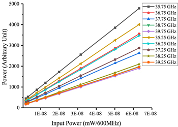
Figure 8. The linearity of the 10 channels. The system linearity is determined according to the power of the broadband white noise signal outputted by the vector signal generator and the value of the digital receiver. The different slopes of the 10 channels are caused by the different gains between the channels.
Download figure:
Standard image High-resolution imageTable 4. The Linearity of the 10 Channels
| Freq. (GHz) | Linearity | Freq. (GHz) | Linearity |
|---|---|---|---|
| 35.25 | 0.99999 | 35.75 | 1 |
| 36.25 | 0.99999 | 36.75 | 0.99999 |
| 37.25 | 0.99999 | 37.75 | 0.99997 |
| 38.25 | 0.99999 | 38.75 | 0.99998 |
| 39.25 | 0.99999 | 39.75 | 0.99999 |
Download table as: ASCIITypeset image
3.3. The Stability of the System
In a real-world observation, fluctuations in the observed data are mainly caused by the target (including the external ambient) and gain fluctuations, so the system stability is tested to distinguish those fluctuations in the observations that may be generated by the instrument rather than the target. Stability was tested in the laboratory at room temperature (without temperature control) and in a real-world environment. The test results show that fluctuations in gain have little effect on the system's counts compared to real-world variations.
First, the gain–temperature relationship was measured, and it can be concluded that the higher the temperature the smaller the gain, and that the temperature control of the system can improve the system stability. The instrument stability is then tested by connecting the first-stage LNA with a 50 Ω terminal instead of the antenna (Figure 9). As shown in Table 5, the coefficient of variation, standard deviation divided by the mean, is less than 0.61% within 9 hr (the range of variation is 2.2%–3.2%).

Figure 9. (a) In the system stability test, the system has poor stability during the first 2.5 hr of instrument operation. With prolonged working, the gain is relatively stable when the heat is volatilized by the conduction-cooling device and the heat generated by the instrument is basically in equilibrium. (b) The gain of the analog unit at different temperatures, including the insertion loss of the test radio frequency cable. An analog signal source (Keysight N5183B) is used as an input and a signal analyzer (Keysight N9040B) reads the output power. Every temperature change is kept in the high–low temperature test chamber for 0.5 hr.
Download figure:
Standard image High-resolution imageTable 5. The Test of System Stability
| No. | Freq. | Average | Standard | Range | Coefficient of |
|---|---|---|---|---|---|
| (GHz) | Deviation | Variation (%) | |||
| 1 | 35.25 | 1153 | 4.441 | 31.3 | 0.39 |
| 2 | 35.75 | 1426 | 5.055 | 36.84 | 0.35 |
| 3 | 36.25 | 944.4 | 3.034 | 22.28 | 0.32 |
| 4 | 36.75 | 1073 | 3.169 | 23.69 | 0.30 |
| 5 | 37.25 | 541.4 | 3.289 | 22.64 | 0.61 |
| 6 | 37.75 | 761.4 | 2.746 | 21.2 | 0.36 |
| 7 | 38.25 | 598.8 | 3.355 | 19.19 | 0.56 |
| 8 | 38.75 | 591 | 2.326 | 16.23 | 0.39 |
| 9 | 39.25 | 530.8 | 2.048 | 14.76 | 0.39 |
| 10 | 39.75 | 562.6 | 1.825 | 12.86 | 0.32 |
Download table as: ASCIITypeset image
The real-world observation is shown in Figure 10. Observations for several days in the period 2021 August 9–September 3 were selected and they were accompanied by various weather conditions such as cloud, rain, rain to clear, and sunny in one day. The variation of output values due to environmental factors is so large that even if the system is calibrated, it should be supplemented by other observation equipment at the same moment to exclude the influence of environmental factors when there is a rise in radiation intensity.
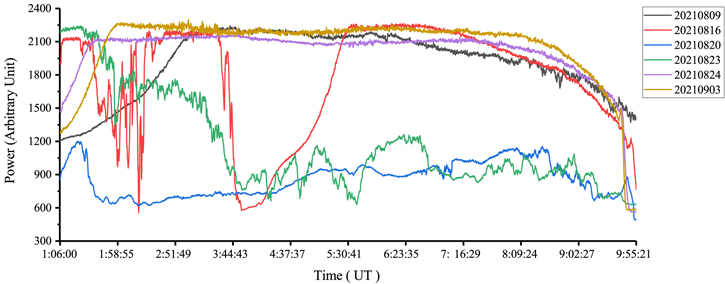
Figure 10. The 35.25 GHz observation data under different weather conditions. Except for August 24 and September 3, which were clear days, the other days were accompanied by different weather conditions. During sunny days, the transient fluctuations are most likely caused by the gain variation, and the small spikes may be caused by the ambience (e.g., clouds). The long-term changes may be caused by the gain fluctuation or the environmental change (e.g., changes in elevation and ambient temperature).
Download figure:
Standard image High-resolution image4. Data Products
Three levels of data products can be supplied by this observing system, i.e., Level 0 (raw data), Level 1 (FITS data), and Level 2 (spectrum and radio flux). Level 0 data is displayed as raw data (binary format) for internal use only. Level 1 data is extracted by removing redundant information from Level 0 data. Level 1 data is given as FITS format files for scientists. Level 2 data is provided in PNG format files for the dynamic spectrum and radio flux intensity (Figure 11).
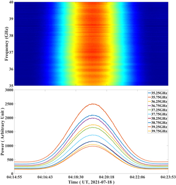
Figure 11. The scan of the Sun. The upper panel shows the spectrum of the 5 GHz bandwidth and the lower panel shows the intensity of the 10 channels.
Download figure:
Standard image High-resolution imageTable 6 shows the relationship between integration, the bandwidth of transmission, time resolution, and coefficient of variation. The large data volume brings huge challenges for storage, as shown by the coefficient of variation of different integration times; the system has a suitable data volume, time resolution, and stability in the default configuration of 1024 accumulations (∼134 ms). The host computer monitors the power of the bandwidth in real time during the display of the spectrum, and after exceeding the power threshold the host computer sends down the parameters to enable the high-time-resolution transmission.
Table 6. The Relationship between Integration, the Bandwidth of Transmission, Temporal Resolution, and Coefficient of Variation
| Number of | Bandwidth | Time | Coefficient of |
|---|---|---|---|
| Accumulations | Resolution | Variation | |
| (Mbps) | (ms) | (%) | |
| 128 | 145.8 | 16.8 | 1.0201 |
| 256 | 72.8 | 33.6 | 0.5692 |
| 512 | 36.3 | 67.1 | 0.3562 |
| 1024 | 18.2 | 134.2 | 0.2306 |
| 2048 | 9.3 | 268.2 | 0.1697 |
| 4096 | 4.7 | 536.6 | 0.1202 |
| 8192 | 2.3 | 1072.4 | 0.086 |
Download table as: ASCIITypeset image
Table 7 gives the main data information of the FITS format. It mainly contains the frequency information of the current packets in the vertical coordinate and the time information of the current packets in the horizontal coordinate. Figure 12 shows the spectrum and radio flux for Level 2 data. The spectrogram is normalized while the system is preheated (Xu et al. 2020). The specifics of the operation are that the observation data divide the average value of 1 minute at the start moment to eliminate the effect of gain. The normalization operation is applied only to the Level 2 data to help find the changes in the spectrum, without changing the Level 1 and Level 0 data.
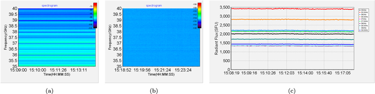
Figure 12. (a) The dynamic spectrum is not consistent under the influence of flatness. (b) After normalization, the dynamic spectrum eliminates the effect of gain. (c) The uncalibrated solar radio flux.
Download figure:
Standard image High-resolution imageTable 7. The Main FITS Header Information for Level 1 Data
| Item Name | Value | Description |
|---|---|---|
| Simple | T | file does conform to FITS standard |
| Bitpix | 16 | number of bits per data pixel |
| Naxis | 2 | number of data axes |
| Naxis1 | 404 | length of data axis 1 |
| Naxis2 | 32780 | length of data axis 2 |
| Origin | SDU Weihai ISS LEAD | organization name |
| Instrume | LCP Cassegrain Antenna | type of instrument |
| Object | Sun | object description |
| Time_OBS | 2021-07-18T03:43:40.643 | date_time observation starts |
| Time_END | 2021-07-18T03:43:54.199 | date_time observation ends |
| Ctype1 | Time [UT] | title of axis 1 |
| Cdelt1 | 134.2178 | step between first and second elements in x-axis (ms) |
| Ctype2 | Frequency [GHz] | title of axis 2 |
| Fre_OBS | 35 GHz | frequency start |
| Fre_END | 40 GHz | frequency end |
| Cdelt2 | 152.532 | step between first and second elements in y-axis (kHz) |
Note. The data header mainly contains information about the antenna, time resolution, frequency resolution, frequency start and end range, etc.
Download table as: ASCIITypeset image
5. Calibration
Based on the previous evaluations of the instrument performance, a rough calibration of the data was therefore performed with a new Moon considering the system can observe the Moon well (Figure 13). Using the new Moon as an external calibration source can eliminate the influence of the receiver's instantaneous instability and the different brightness temperatures at different zenith angles (Kallunki & Tornikoski 2018; Yan et al. 2021).

Figure 13. (a) The 5 GHz bandwidth dynamic spectrum for the Sun and the Moon where the flatness is optimized. The spectra of dark blue, light blue, and yellow are the background of the sky, the Moon, and the Sun, respectively. (b) The radiation intensity of the Sun and the Moon corresponding to (a).
Download figure:
Standard image High-resolution imageDuring each calibration operation, the antenna pointed to the Sun (TSun), the Sun background (Tbks), the Moon (TMoon) and the Moon background (Tbkm) in turn, and the corresponding ratio (R) among them is calculated by

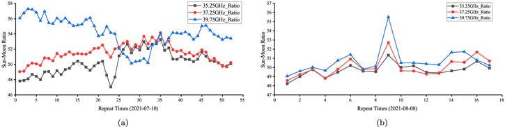
By the new Moon calibration, as shown in Figure 14, the average of the ratio at 35.25, 37.25, and 39.75 GHz are about 49.9, 51.3, and 54.2 on July 10, and 49.7, 50.1, and 50.7 on August 8, respectively. The results show that the Sun–Moon ratio varies from 43.1–53.3 for 35.25 GHz, 47.1–54.2 for 37.25 GHz, and 49–57.3 for 39.75 GHz. The corresponding new Moon temperatures at 35.25, 37.25, and 39.75 GHz are 245.5, 246.1, and 248 K, respectively (Kuseski & Swanson 1976; Pelyushenko & Chernyshev 1983; Hafez et al. 2014). So the solar brightness temperature is measured to be 10,581.1–13,085.2, 11,591.3–13,338.6, and 12,152–14,210.4 K at these points. These ratios are close to the theoretical ratios, but do not distinguish well between the different frequency ratios. Calibration is influenced by the external environment, the time interval during the calibration operation, the instrument itself (for example, a small antenna diameter leads to a slight difference between the Moon and Moon background, which is more susceptible to the ambient environment), and other factors.
Figure 14. Solar radio flux intensity was calibrated by using the new Moon on 2021 July 10 and August 8. Since the difference between the Moon and Moon background is small, the small fluctuations in the observation lead to a large difference in the Sun-to-Moon ratio.
Download figure:
Standard image High-resolution image
6. Conclusion and Discussion
To obtain microwave observation with a complete frequency coverage, we designed and developed a commonly used solar radio observing system which can work from several to tens of gigahertz. This system has been tested and used for solar microwave observation in the frequency range of 35–40 GHz at CSO for more than 1 yr. According to our test, the performance parameters of the solar radio telescope are obtained as follows: an observation bandwidth of 5 GHz, an instantaneous observation bandwidth of 1 GHz, a time resolution of about 134 ms (routine observation), a frequency resolution of 153 kHz, a data bandwidth of 18.2 Mbps at 134 ms, linearity better than 0.9999, and the Sun-to-Moon ratio of 43.1–53.3 was obtained at 35.25 GHz through new Moon calibration.
Based on observations over one year, we find that improvement should be made in the future. As we can see that the environmental temperature can play an important role in a long-term observation (Figure 10), a temperature control system is urgently needed to be developed. Moreover, the new Moon calibration needs further improvements in accuracy due to the instrument and environmental effects, and we will research the absolute calibration theory to implement the calibration of the 35–40 GHz solar radio flux in the next step.
This research was supported by the National Natural Science Foundation of China (41774180, 41904158, 11703017), the China Postdoctoral Science Foundation (2019M652385), the Shandong postdoctoral innovation project (202002004), and the Young Scholars Program of Shandong University, Weihai (20820201005).