


Abstract
The goals of this study are (1) to test the best theoretical transition probabilities for Ca i (a relatively light alkaline earth spectrum) from a modern ab initio calculation using configuration interaction plus many-body perturbation theory against the best modern experimental transition probabilities and (2) to produce as accurate and comprehensive a line list of Ca i transition probabilities as is currently possible based on this comparison. We report new Ca i radiative lifetime measurements from a laser-induced fluorescence experiment and new emission branching fraction measurements from a 0.5 m focal length grating spectrometer with a detector array. We combine these data for upper levels that have both a new lifetime and new branching fractions to report log(gf) values for two multiplets consisting of nine transitions. Detailed comparisons are made between theory and experiment, including the measurements reported herein and a selected set of previously published experimental transition probabilities. We find that modern theory compares favorably to experimental measurements in most instances where such data exist. A final list of 202 recommended transition probabilities is presented, which covers lines of Ca i with wavelengths ranging from 2200 to 10000 Å. These are mostly selected from theory but are augmented with high-quality experimental measurements from this work and from the literature. The recommended transition probabilities are used in a redetermination of the Ca abundance in the Sun and in the metal-poor star HD 84937.
Export citation and abstract BibTeX RIS
1. Introduction
The story of early Galactic nucleosynthesis begins with detailed chemical compositions of low-metallicity Milky Way halo stars. The record of the initial burst of massive star births, very short lives, and violent deaths is written in the abundance distributions of metal-poor stars. We must try to decode the abundance data to make any sense of how the Milky Way was born. But first we must determine the abundances accurately to have any hope of progressing beyond general guesses about what the early Galaxy did, when, how, and where.
Derivation of stellar abundances depends on many factors, from obtaining excellent high-resolution spectra, to constructing trustworthy stellar atmospheric models, to computing line absorption profiles with realistic radiative transfer techniques. But the efforts in these areas will be useless without high-quality line transition data. In particular, absolute atomic transition probabilities, or log(gf) values, are critical to elemental abundance studies. Additionally, improved data on hyperfine and/or isotopic structure, as well as improved energy levels, are also vital, especially in cases where lines are saturated and/or blended.
In this paper we report improved transition probabilities for the first spectrum of the light "α"-element calcium. 7 Several α-elements can be detected in very metal-poor stars: O, Mg, Si, S, and Ca. Their synthesis in massive stars has been understood for decades. However, these elements have generally not enjoyed recent comprehensive laboratory studies to the same degree as the Fe-group or neutron-capture elements. Ca is a relatively light alkaline earth, with small relativistic effects and with only two valence electrons. It is reasonable to hypothesize that for Ca i modern theory should be as accurate as modern experimental techniques. This hypothesis is tested in our work. There are a number of theoretical studies of Ca i in the literature. We choose the comprehensive work of Mills et al. (2017, hereafter M17) to make a detailed comparison to modern experiments.
Section 2 of this paper contains a brief summary of recent theoretical calculations of Ca i, followed by a comparison of experimental radiative lifetime measurements to theoretical lifetimes derived from M17. New laser-induced fluorescence (LIF) lifetime measurements, accurate to 5%, are reported in Section 2. Published measurements from LIF and other laser-based measurements are also included in the comparison. Section 3 of this paper is a comparison of emission branching fractions (BFs) from our laboratory measurements and from the published literature to theoretical BFs from M17. In Section 3.4 we present new log(gf) values for nine transitions from two multiplets. Also discussed in Section 3 is our further development of calibration techniques based on a standard detector. A set of recommended log(gf) values for lines of Ca i is reported in Section 4. The recommended list of log(gf) values includes theoretical values from M17 and selected sets of measurements with some renormalization. In Section 5 this list of recommended lines is used to redetermine the Ca abundance in the Sun and metal-poor star HD 84937. Finally, Section 6 includes a summary and some conclusions.
2. Radiative Lifetimes—Theory and Experiment
As noted above, neutral Ca is an alkaline earth with two valence electrons outside of a closed shell. These valence electrons yield an array of singlet and triplet levels. Spin–orbit splitting is a relativistic effect that is small in Ca i because of calcium's relatively light weight. This type of structure is also called LS or Russell–Saunders coupling. Figure 1 is a partial Grotrian diagram of Ca i that illustrates this singlet/triplet structure. (Note that in this figure the splitting between levels in a triplet term is exaggerated for the purposes of illustration.) Also shown in Figure 1 are the transition multiplets studied in the BF measurements described later in Section 3 (black lines connecting terms), as well as the multiplets studied in other experimental work (colored lines connecting terms) that we draw on in Section 4 to generate our recommended list of log(gf) values. This figure should help the reader visualize the structure and related transitions in the detailed discussions below in the laboratory Sections 3 and 4.
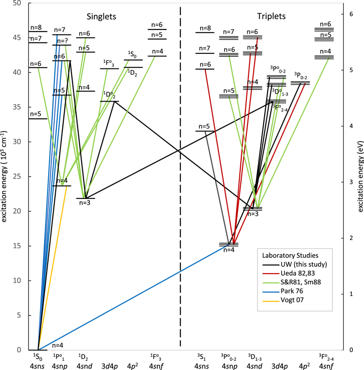
Figure 1. Partial Grotrian diagram of Ca i showing all but two high-lying configurations considered by M17. Configuration (and term where applicable to entire column) of each vertical set of levels is given along the bottom axis. The singlet/triplet structure is illustrated. The diagram is to scale in the vertical direction except for the spacing of the levels in each triplet, which is exaggerated for the purpose of illustration. Also shown are lines connecting terms that indicate the transition multiplets from experimental studies discussed in the text. Legend abbreviations: UW—this study; Ueda 82,83—Ueda et al. (1982) and Ueda et al. (1983); S&R81—Smith & Raggett (1981); Sm88—Smith (1988); Park 76—Parkinson et al. (1976); Vogt 07—Vogt et al. (2007).
Download figure:
Standard image High-resolution image2.1. Recent Theoretical Studies of Ca i
There have been a handful of quality theoretical calculations of Ca i in the past two decades. The Notre Dame team (e.g., Savukov & Johnson 2002) used the configuration interaction plus many-body perturbation theory (CI+MBPT) method in an ab initio computation to find a small number of log(gf) values, including transition probabilities for five spin-allowed resonance lines 8 and six spin-forbidden resonance lines. A larger calculation for neutral Ca was published by the Vanderbilt team (e.g., Froese-Fischer & Tachiev 2003) using the multiconfiguration Hartree–Fock (MCHF) method, which included all levels up to the 3d4p1F3. Transition probabilities were reported for ∼24 spin-allowed lines and a smaller number of spin-forbidden lines. Most recently, M17 used the ab initio CI+MBPT method to compute transition probabilities for over 800 electric-dipole transitions of Ca i, including most spin-allowed lines of interest and some spin-forbidden lines. Because of the comprehensiveness of this study, we have selected the work of M17 to test against our new measurements and other published measurements using modern methods.
The M17 data, which are included as supplemental material in that publication, are not in a user-friendly format, as they require proprietary software to easily access. Unfortunately, the republication of the data by Yu & Derevianko (2018) has a few errors from misidentification of Rydberg levels. It has been recommended by an author that the supplemental material of M17 be used to resolve any discordance (A. Derevianko 2021, private communication). There are no uncertainties quoted either in M17 or in the republication of the data by Yu & Derevianko. The latter publication does at least provide both the length and velocity forms of the calculation, as well as the percent difference between them (L−V) for many of the transitions studied. They found that the length form agreed better when compared to experiment and recommended that form, but they found that for stronger lines the two forms agreed within a few percent. This L−V comparison can be used as a rough gauge of the theoretical uncertainties. Ca has attracted the attention of both theorists and experimentalists for decades, and thus we omit comparisons to some of the older 208 publications on Ca i in the bibliography of the National Institute of Standards and Technology (NIST) Atomic Spectra Database (ASD) (Kramida et al. 2019). Results in many of the older publications have larger error bars than more recent studies. Our goal is to test the M17 theoretical results against the highest-quality modern experimental results.
The M17 study was motivated by possible use of Ca in an optical frequency standard clock. Although microwave frequency clocks tied to a hyperfine transition of Cs are used as standard clocks today, it is anticipated that at some time those microwave frequency clocks will be replaced by optical frequency clocks. Very narrow optical transitions, when used for locking a clock oscillator, have the potential to make a standard clock with far greater (at least a million fold) accuracy and precision than can be achieved using a microwave transition. The same laser-cooled atom technology used in atomic clocks can be applied to transition probability measurements on certain resonance lines. Vogt et al. (2007) built on the work of Zinner et al. (2000) and Degenhardt et al. (2003) to measure the transition probability of the λ4226.728 resonance line of Ca i, from the upper 4s4p1P°1 to ground-state 4s2 1S0 level, with an estimated accuracy and precision of ±0.04%. This transition is indicated in Figure 1 with an orange line. (The transition probability of this Ca i spin-allowed resonance line was already known to a few percent accuracy and precision, which is adequate for most astrophysical research.) The laser-cooled atom technique is not broadly applicable to the many other optical and ultraviolet (UV) transitions of Ca i. However, the extensive theoretical work on >800 lines of Ca i in M17 is of great utility to astrophysics and to other fields.
2.2. Experimental Radiative Lifetimes
Radiative lifetimes are measured using time-resolved LIF spectroscopy on neutral Ca atoms in a slow atomic beam produced in an electric discharge sputter source. This experiment has been successfully applied to many neutral and singly ionized species throughout the periodic table over nearly four decades, and hence has been described many times in print. Here we will give a somewhat cursory description of the experimental technique. The reader is referred to Den Hartog et al. (2002) for a more detailed description of the experiment and an in-depth discussion of the various systematic effects associated with the measurements and how they are mitigated.
A gas-phase sample of Ca atoms is produced by sputtering in a pulsed hollow cathode discharge operating with 30 mA DC and 5–10 A, 10 μs pulses in ∼0.4 torr argon. The hollow cathode is closed on the downstream end except for a 1 mm hole through which the beam exits. The cathode is made of steel and is typically lined with a high-purity thin sheet of whatever metal is being studied. Calcium, however, is very reactive and oxidizes so readily that it is not generally available in sheet form. Instead, we had an 80% Al/20% Ca alloy disk manufactured to line the bottom of the cathode and used 1100 aluminum shim stock to line the vertical walls of the cathode. The alloy was chosen because it is much less reactive than pure Ca and therefore easier to sputter off the oxide layer during cathode conditioning. The Ca atoms and ions exit the cathode through the 1 mm hole, entrained in a flow of argon gas, into a scattering chamber that is held at ∼1 × 10⁻⁴ torr. The atomic beam environment has been tested and repeatedly shown to be free from effects related to collisional depopulation and optical depth. This beam of Ca atoms is slow (∼5 × 104 cm s−1) and weakly collimated and has a mix of ground and metastable level populations. In neutral Ca, the ground level is a 4s2 1S0 and the lowest metastable levels are in the 4s4p3P° term at ∼15,000 cm−1 (see Figure 1). Using these populations as lower levels, we have access to odd-parity 1P° terms, as well as even-parity 3S, 3P, and 3D terms using single-step laser excitation. The even-parity 4s4d1D2 metastable level at 21,849 cm−1 is too weakly populated in our beam to make use of as the lower level of a single-step excitation.
A laser beam intersects the atomic beam at right angles 1 cm below the bottom of the cathode and is used to selectively excite the level being studied. Selective excitation is an important advantage of laser-based lifetime measurements. Older techniques that relied on nonselective electron beam excitation were prone to systematic error due to cascade from higher-lying levels. The laser used in this study is a pulsed dye laser pumped with a nitrogen laser. It has a bandwidth of ∼0.2 cm−1 and is tunable from ∼2050 to 7000 Å using a variety of dyes and frequency doubling crystals. The laser pulse is ∼3 ns duration and terminates completely within a few nanoseconds of peak intensity. This abrupt termination makes it possible to record the fluorescence decay free from laser interaction. The laser is triggered 20–30 μs after the peak of the discharge current, allowing transit time for the atoms to reach the beam interaction region. Light from the laser is polarized along the axis of the atomic beam, resulting in the possibility of Zeeman quantum beats. This is a phenomenon that arises because the excitation from the polarized laser leaves the atoms in a dipole-aligned state. These dipoles then precess about Earth's magnetic field while radiating, sweeping the nonuniform dipole radiation pattern through the direction of view, resulting in an oscillation of the fluorescence signal. To mitigate this effect, the field is zeroed to within ±0.02 G in the viewing volume using a set of Helmholtz coils. When long lifetimes (>300 ns) are measured, a high magnetic field (30 G) is imposed along the laser axis so that the precession is very fast relative to the timescale of the measurement, and the oscillations in the fluorescence average away. The longest Ca i lifetime measured in this study is <50 ns, so the high field was not required.
Fluorescence is collected in a direction perpendicular to the plane defined by the laser and atom beams. A pair of fused silica lenses are used to image the beam interaction region with unity magnification onto the photocathode of an RCA 1P28A photomultiplier tube (PMT). Optical filters, either broadband colored glass filters or narrowband multilayer dielectric filters, are often placed between the two lenses, where the fluorescence is roughly collimated in order to block scattered laser light, as well as cascade radiation from lower-lying levels. Occasionally, for the measurement of long lifetimes, it is also necessary to place a cylindrical lens between the two fluorescence collection lenses to defocus the light at the PMT. This is to mitigate the flight-out-of-view effect, in which the image of atoms fluorescing later in the decay has moved to a region of lower sensitivity on the PMT photocathode, resulting in a perceived shortening of the lifetime. The flight-out-of-view effect only becomes a problem for lifetimes longer than 300 ns for neutral atoms and 100 ns for ions, which move somewhat faster in the beam, and thus was not an issue in our measurement of the Ca i lifetimes in this study.
The PMT has a rise time of ∼1.7 ns, and the electrode chain is carefully wired for low inductance to minimize ringing. The PMT signal is put through a high-bandwidth 60 ns delay line and into a Tektronix SCD1000 transient digitizer for signal recording. The bandwidth and fidelity of the detection electronics are such that only lifetimes below 3 ns show any systematic distortion. The shortest lifetime we have measured in Ca i is 4.6 ns, well above this limit. Another systematic arising from the PMT is caused by an after-pulse signal. After-pulsing arises from an imperfect vacuum within the PMT. As the fast electron avalanche proceeds from photocathode to anode, some ionization of residual gas in the PMT occurs. These ions make their way toward the cathode, but on a much longer timescale given the much higher mass of the ions compared to that of the electrons. The result is a very weak pulse ∼150 ns after the fast pulse and spread over tens of nanoseconds. This effect results in a lengthening of lifetimes in the 100–150 ns range by a few percent. This effect can be reduced by periodically introducing a light leak into the optical system for a number of hours resulting in a 1 μA DC PMT anode current that causes the ionized gas to be buried in the cathode. This "degassing" of the PMT does not eliminate the effect altogether but reduces it substantially.
The desired transition wavelength is found by first coarse tuning the laser wavelength to within ∼0.5 Å as measured by a 0.5 m focal length monochromator. Coarse tuning is accomplished by tipping the grating, which is the tuning element of the dye laser. An LIF spectrum is then recorded over a 5–10 Å range by slowly changing the pressure of nitrogen in an enclosed volume surrounding the grating. This "pressure scanning" gives very fine and reproducible control of the laser wavelength. Data acquisition involves recording an average of 640 fluorescence decays, starting only after the laser has completely terminated and for a time span equivalent to approximately three lifetimes. The laser is then tuned off the transition, and an average of 640 backgrounds is recorded. The lifetime is determined, for both early time (first half of the trace) and late time (second half of the trace), by doing a least-squares fit to a single exponential on the difference between the signal and background records. Comparison of the early and late lifetimes is a quick and sensitive way to determine if the decay is a clean exponential or if it has some distortion from a systematic effect, such as cascade radiation through lower levels, that needs further study. A set of five of these acquisitions and analyses comprise one lifetime determination. The lifetime is determined twice for each upper level using a different laser transition whenever possible. This redundancy helps to ensure that the transitions are identified correctly in the experiment, that they are correctly classified to the level, and that neither transition is blended.
Systematic effects in the experiment are well understood and controlled at the ±5% level, which is our quoted uncertainty in most cases. To ensure that our experiment is operating reproducibly and our measurements lie within the stated uncertainties, we routinely measure a set of "benchmark" lifetimes. These are lifetimes that are accurately known from other sources and have been determined either from theory or from an experiment with different and smaller systematic uncertainties than in our experiment. To cover the range of lifetimes measured for Ca i, we have measured the following benchmark lifetimes: 22P1/2,3/2 levels of Ca+ at 6.904(26) ns (Hettrich et al. 2015) and 6.639(42) ns (Meir et al. 2020), respectively; the 22P3/2 level of Be+ at 8.8519(8) ns (variational method calculation, Yan et al. 1998); the 32P3/2 level of neutral Na at 16.23(1) ns (NIST critical compilation of Kelleher & Podobedova 2008 uncertainty of ±0.1% at 90% confidence level); and the 4p'[1/2]1 level of neutral Ar at 27.85(7) ns (beam-gas-laser-spectroscopy, Volz & Schmoranzer 1998). We also note that our remeasurement of the Ca 4s4p1P1 lifetime similarly acts as a "benchmark" end-to-end check of our experiment, as this lifetime is known to very high accuracy and precision from other sources (e.g., Vogt et al. 2007).
The results of our radiative lifetime measurements are given in Table 1, along with all other experimental lifetimes measured using LIF or other modern laser-based methods. In addition, we compare to lifetimes determined from the theoretical transition probabilities of M17. We do not include comparisons to older experimental methods that involved nonselective excitation. Configurations, terms, and level energies in Table 1 and in subsequent text, tables, and figures are taken from the NIST ASD (Kramida et al. 2019). Air wavelengths used throughout the text and tables are calculated using these energy levels and the index of air from Peck & Reeder (1972).
Table 1. Radiative Lifetimes for Levels of Neutral Ca
| Level | Radiative Lifetimes (ns) | |||||||||
|---|---|---|---|---|---|---|---|---|---|---|
| Configuration a | Term a | Energy a (cm−1) | UW b | M17 Theory | Havey et al. (1977) | Hansen (1983) | Aldenius et al. (2009) | Jönsson et al. (1984) | Other | Other References |
| 3p64s4p | 1P°1 | 23652.304 | 4.64 ± 0.23 | 4.6 | 4.7 ± 0.5 | 4.6 ± 0.2 | ⋯ | ⋯ | 4.6386 ± 0.0017 | 1 |
| ⋯ | ⋯ | ⋯ | ⋯ | ⋯ | ⋯ | ⋯ | ⋯ | ⋯ | 4.65 ± 0.04 | 2 |
| ⋯ | ⋯ | ⋯ | ⋯ | ⋯ | ⋯ | ⋯ | ⋯ | ⋯ | 4.49 ± 0.07 | 3 |
| ⋯ | ⋯ | ⋯ | ⋯ | ⋯ | ⋯ | ⋯ | ⋯ | ⋯ | 4.6 ± 0.2 | 4 |
| 3p64s5s | 3S1 | 31539.495 | 12.3 ± 0.6 | 12.1 | 11.7 ± 0.6 | ⋯ | 13.8 ± 1.2 | ⋯ | 10.7 ± 1.0 | 5 |
| ⋯ | ⋯ | ⋯ | ⋯ | ⋯ | ⋯ | ⋯ | ⋯ | ⋯ | 12.4 ± 0.5 | 6 |
| 3p64s4d | 1D2 | 37298.287 | ⋯ | 62.3 | 80.2 ± 9.6 | ⋯ | ⋯ | ⋯ | 63 ± 10 | 7 |
| 3p64s4d | 3D1 | 37748.197 | 12.2 ± 0.6 | 12.7 | ⋯ | ⋯ | 13.6 ± 1.0 | 13.0 ± 0.5 | 12.3 ± 1.0 | 5 |
| ⋯ | 3D2 | 37751.867 | 12.2 ± 0.6 | 12.8 | ⋯ | ⋯ | 14.1 ± 1.1 | 13.0 ± 1.5 | ⋯ | ⋯ |
| ⋯ | 3D3 | 37757.449 | 12.3 ± 0.6 | 12.8 | ⋯ | ⋯ | 15.4 ± 1.2 | 13.0 ± 2.5 | ⋯ | ⋯ |
| 3p64p2 | 3P0 | 38417.543 | 5.80 ± 0.29 | 5.5 | ⋯ | ⋯ | ⋯ | 6.9 ± 0.4 | ⋯ | ⋯ |
| ⋯ | 3P1 | 38464.808 | 5.63 ± 0.28 | 5.5 | ⋯ | ⋯ | ⋯ | 6.9 ± 0.4 | ⋯ | ⋯ |
| ⋯ | 3P2 | 38551.558 | 5.66 ± 0.28 | 5.5 | ⋯ | ⋯ | ⋯ | 6.9 ± 0.4 | ⋯ | ⋯ |
| 3p64s6s | 3S1 | 40474.241 | 31.7 ± 1.6 | 30.6 | ⋯ | ⋯ | ⋯ | ⋯ | ⋯ | ⋯ |
| 3p63d4p | 1F°3 | 40537.893 | ⋯ | 137.3 | ⋯ | ⋯ | ⋯ | ⋯ | 58.3 ± 2 | 8 |
| 3p64s6s | 1S0 | 40690.435 | ⋯ | 142.0 | 88.9 ± 3.0 | ⋯ | ⋯ | ⋯ | ⋯ | ⋯ |
| 3p64p2 | 1D2 | 40719.847 | ⋯ | 16.9 | 14.9 ± 0.9 | ⋯ | ⋯ | 16.3 ± 2.0 | 14.47 ± 0.14 | 7 |
| 3p64s6p | 1P°1 | 41679.008 | 20.6 ± 1.0 | 27.7 | ⋯ | ⋯ | ⋯ | ⋯ | ⋯ | ⋯ |
| 3p64p2 | 1S0 | 41786.276 | ⋯ | 12.6 | 12.6 ± 0.8 | ⋯ | ⋯ | 14.4 ± 0.7 | ⋯ | ⋯ |
| 3p64s4f | 1F°3 | 42343.587 | ⋯ | 26.4 | ⋯ | ⋯ | ⋯ | ⋯ | 24.6 ± 1.4 | 9 |
| 3p64s5d | 3D1 | 42743.002 | 24.8 ± 1.2 | 24.7 | ⋯ | ⋯ | 27.0 ± 2.0 | ⋯ | ⋯ | ⋯ |
| ⋯ | 3D2 | 42744.716 | 24.9 ± 1.2 | 24.7 | ⋯ | ⋯ | 27.0 ± 2.0 | ⋯ | ⋯ | ⋯ |
| ⋯ | 3D3 | 42747.387 | 24.9 ± 1.2 | 24.8 | ⋯ | ⋯ | 27.0 ± 2.0 | ⋯ | ⋯ | ⋯ |
| 3p64s5d | 1D2 | 42919.053 | ⋯ | 19.6 | 22.2 ± 1.3 | ⋯ | ⋯ | ⋯ | 21.3 ± 0.7 | 7 |
| 3p64snp | w1P°1 | 43933.477 | 15.7 ± 0.8 | 13.2 | ⋯ | ⋯ | ⋯ | ⋯ | ⋯ | ⋯ |
| 3p64s7s | 1S0 | 44276.538 | ⋯ | 92.5 | 62.4 ± 4.3 | 63.4 ± 2.9 | ⋯ | ⋯ | ⋯ | ⋯ |
| 3p64s5f | 1F°3 | 44804.878 | ⋯ | 43.3 | ⋯ | ⋯ | ⋯ | 60 ± 3 | 62.1 ± 2 | 9 |
| 3p64s6d | 1D2 | 44989.830 | ⋯ | 91.7 | ⋯ | 58.9 ± 2.5 | ⋯ | ⋯ | ⋯ | ⋯ |
| 3p64s7p | 1P°1 | 45425.358 | 43.3 ± 2.2 | 43.7 | ⋯ | ⋯ | ⋯ | ⋯ | ⋯ | ⋯ |
| 3p64s8s | 1S0 | 45887.200 | ⋯ | 156.7 | 118.3 ± 6.3 | 124.9 ± 6.0 | ⋯ | ⋯ | ⋯ | ⋯ |
| 3p64s6f | 1F°3 | 46182.399 | ⋯ | 96.7 | ⋯ | ⋯ | ⋯ | ⋯ | 99 ± 4 | 9 |
| 3p64s7d | 1D2 | 46200.13 | ⋯ | ⋯ | ⋯ | 224 ± 12 | ⋯ | ⋯ | ⋯ | ⋯ |
| 3p64s9s | 1S0 | 46835.055 | ⋯ | ⋯ | ⋯ | 206 ± 11 | ⋯ | ⋯ | ⋯ | ⋯ |
| 3p64s10s | 1S0 | 47437.471 | ⋯ | ⋯ | ⋯ | 294 ± 17 | ⋯ | ⋯ | ⋯ | ⋯ |
| 3p63d5s | 1D2 | 47449.083 | ⋯ | ⋯ | ⋯ | 81.2 ± 6.9 | ⋯ | ⋯ | ⋯ | ⋯ |
| 3p64s9d | 1D2 | 47812.39 | ⋯ | ⋯ | ⋯ | 232 ± 12 | ⋯ | ⋯ | ⋯ | ⋯ |
| 3p64s11s | 1S0 | 47843.76 | ⋯ | ⋯ | ⋯ | 420 ± 29 | ⋯ | ⋯ | ⋯ | ⋯ |
| 3p64s10d | 1D2 | 48083.41 | ⋯ | ⋯ | ⋯ | 271 ± 16 | ⋯ | ⋯ | ⋯ | ⋯ |
| 3p64s12s | 1S0 | 48130.75 | ⋯ | ⋯ | ⋯ | 594 ± 46 | ⋯ | ⋯ | ⋯ | ⋯ |
| 3p64s11d | 1D2 | 48290.85 | ⋯ | ⋯ | ⋯ | 425 ± 36 | ⋯ | ⋯ | ⋯ | ⋯ |
| 3p64s13s | 1S0 | 48340.75 | ⋯ | ⋯ | ⋯ | 808 ± 72 | ⋯ | ⋯ | ⋯ | ⋯ |
| 3p64s14s | 1S0 | 48499.14 | ⋯ | ⋯ | ⋯ | 720 ± 65 | ⋯ | ⋯ | ⋯ | ⋯ |
| 3p63d2 | 3P2 | 48563.522 | 8.7 ± 0.4 | ⋯ | ⋯ | ⋯ | ⋯ | ⋯ | ⋯ | ⋯ |
Notes.
a Configuration, term, and level energy from NIST ASD (Kramida et al. 2019). b The uncertainty on all UW lifetimes (present study) is ±5%.Other References. (1) Vogt et al. 2007; (2) Degenhardt et al. 2003; (3) Kelly & Mathur 1980; (4) Hannaford & Lowe 1981; (5) Gornik et al. 1973; (6) Major et al. 1985; (7) Hunter et al. 1985; (8) Hunter & Peck 1986; (9) Bhatia 1986.
Download table as: ASCIITypeset image
3. Emission Branching Fractions and log(gf) Values
The combination of radiative lifetimes from LIF measurements with emission BFs from Fourier transform spectrometers (FTSs) or other high-resolution spectrometers has proven to be an efficient and accurate method for measuring A-values and log(gf) values (e.g., Lawler et al. 2009). The radiative lifetime of an upper level u provides the absolute scale when converting the BFs of transitions connected to that level to A-values. The BF for a transition between u and a lower level l is the ratio of its A-value to the sum of the A-values for all transitions associated with u, which is the inverse of the radiative lifetime, τu . This can also be expressed as the ratio of relative emission intensities I (in any units proportional to photons/time) for these transitions:
BFs, by definition, sum to unity, or near unity if a few residual weak lines are not measured. It is therefore important when measuring BFs to account for all possible decay paths from an upper level so that the normalization is correct. If some significant transitions are omitted, then one has a branching ratio (BR) rather than a BF.
3.1. BFs of Triplet Multiplets
Triplet multiplets—the transitions connecting the levels in an upper triplet term to those in a lower triplet term—typically are spread over one or at most a few percent fractional change in wavelength owing to the close spacing of levels in each term. The emission BF measurements on triplet multiplets reported herein were made using a Jarrell-Ash 0.5 m focal length grating spectrometer equipped with a 1180 groove mm−1 diffraction grating blazed for 3000 Å. The grating spectrometer was equipped with an Si photodiode array having 1024 pixels, each 25 μm wide. An internal relative radiometric calibration technique employing Ar i and Ar ii lines (Whaling et al. 1993) has been used heavily by our group in the analysis of FTS data from other species. This technique is desirable when calibrating spectra over wide wavelength ranges because it captures wavelength-dependent effects such as window transmission and internal reflections in the lamp source. The minimal wavelength spread of the multiplets studied here negates the need for this method, and an external calibration is used herein. The spectrometer and detector array are calibrated over the small wavelength ranges needed using an NIST traceable tungsten-quartz-halogen (WQH) standard lamp operated at 6.5 amps.
Table 2 reports our emission BF measurements on a triplet multiplet from the upper 4s5s3S1 level to the 4s4p3P° term. These are true BFs with residuals ≪0.01. Comparisons of our measurements to BF measurements from Aldenius et al. (2009), to theoretical BFs from M17, and to pure LS (see, e.g., Appendix I of Cowan 1981 for the tabulation of LS intensities from perturbation theory) are included in Table 2. Emission BFs for this particular multiplet, as measured in the present study and by Aldenius et al., are found to be a nearly pure triplet that follows predicted LS BFs to a good approximation. This can be seen in Figure 2(a), where we plot the difference of log(BF) between our results and those of M17 versus the M17 BFs. In panel (a), we also make the same comparison between LS BFs and those of M17. In this plot, as well as in panels (b)–(e), the horizontal line at 0.00 indicates perfect agreement with the M17 calculations. The same multiplet was studied earlier using absorption spectroscopy by Smith & O'Neill (1975), who also found nearly pure LS results. Similarly, Table 3 reports our emission BF measurements on a triplet multiplet from the upper 4p2 3P term to the 4s4p3P° term. Again, these are true BFs with residuals ≪0.01. Comparisons of our measurements to theoretical BFs from M17 and pure LS BFs are given in Table 3 and plotted in Figure 2(b). As with the previous multiplet, both experiment and theory show extremely good agreement with simple LS coupling theory.
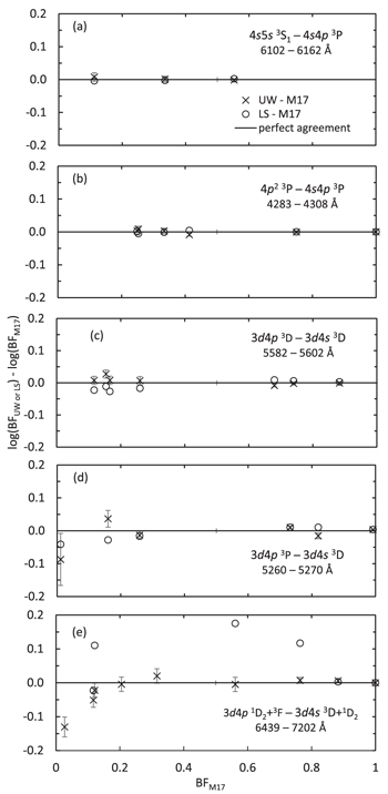
Figure 2. Logarithmic comparison of measured (UW) and LS theory BFs with those of M17. The crosses indicate log(BF) differences between this study (UW) and M17, and open circles indicate those differences between LS theory and M17. The solid horizontal line corresponds to perfect agreement with M17. Panels (a)–(e) present the data of Tables 2–6, respectively. All panels are displayed with the same vertical scale to emphasize that neutral Ca obeys LS coupling to a high degree (panels (a)–(d)), and where there is a divergence from LS theory due to mixing of levels (panel (e)), M17 has calculated that mixing accurately.
Download figure:
Standard image High-resolution imageTable 2. Emission BF Measurements on a Multiplet from the Upper 4s5s3S1 Level to the 4s4p3P Term
| Eupp | Jupp | Elow | Jlow | λair | BF | Unc. | BF | Unc. | BF | BF |
|---|---|---|---|---|---|---|---|---|---|---|
| (cm−1) | (cm−1) | (Å) | This Expt. | (%) | A09 a | (%) | M17 | Pure LS b | ||
| 31539.495 | 1 | 15157.901 | 0 | 6102.7227 | 0.114 | 3 | 0.115 | 3 | 0.112 | 0.111 |
| 31539.495 | 1 | 15210.063 | 1 | 6122.2172 | 0.336 | 2 | 0.339 | 2 | 0.335 | 0.333 |
| 31539.495 | 1 | 15315.943 | 2 | 6162.1730 | 0.551 | 1 | 0.546 | 2 | 0.553 | 0.556 |
Notes.
a A09: Aldenius et al. (2009). b LS BFs are calculated from perturbation theory. See, e.g., Appendix I of Cowan (1981) for a tabulation of LS line strengths.Download table as: ASCIITypeset image
Table 3. Emission BF Measurements on a Multiplet from the Upper 4p2 3P Term to the 4s4p3P Term
| Eupp | Jupp | Elow | Jlow | λair | BF | Unc. | BF | BF |
|---|---|---|---|---|---|---|---|---|
| (cm−1) | (cm−1) | (Å) | This Expt. | (%) | M17 | Pure LS | ||
| 38417.543 | 0 | 15210.063 | 1 | 4307.7439 | 1.000 | 0 | 1.000 | 1.000 |
| 38464.808 | 1 | 15157.901 | 0 | 4289.3668 | 0.336 | 2 | 0.334 | 0.333 |
| 38464.808 | 1 | 15210.063 | 1 | 4298.9883 | 0.258 | 2 | 0.253 | 0.250 |
| 38464.808 | 1 | 15315.943 | 2 | 4318.6517 | 0.405 | 1 | 0.413 | 0.417 |
| 38551.558 | 2 | 15210.063 | 1 | 4283.0106 | 0.251 | 3 | 0.249 | 0.250 |
| 38551.558 | 2 | 15315.943 | 2 | 4302.5278 | 0.749 | 1 | 0.750 | 0.750 |
Download table as: ASCIITypeset image
Results presented in Tables 2 and 3 and Figures 2(a) and (b) are for even-parity upper triplet terms. It is reasonable to check a few odd-parity upper triplet terms. Table 4 reports our emission BF measurements on a triplet multiplet from the upper 3d4p3D° term to the 3d4s3D term. These are true BFs with residuals <0.01 as indicated by the BFs from M17. Table 4 includes a comparison of our measurements to theoretical BFs from M17 and to pure LS BFs, and these comparisons are presented also in Figure 2(c). As can be seen in the figure, this multiplet also follows LS BFs to a good approximation, although not quite as closely as the previous two even-parity multiplets. This multiplet was studied earlier using absorption spectroscopy by Smith & Raggett (1981), who also found nearly pure LS results. Nearby levels of the same parity and J of the upper levels of this multiplet can "repel" triplet levels of the upper term and help explain the small deviations between pure LS BFs and those calculated by M17. Finally, Table 5 reports our emission BF measurements on a triplet multiplet from the upper 3d4p3P° term to the 3d4s3D term. For measurement of the weakest line of the multiplet, an echelle grating was substituted for the first order grating in the Jarrell-Ash 0.5 m spectrometer in order to increase the instrument resolving power so as to isolate the line from nearby stronger lines. These are true BFs with residuals of ∼0.008 to 0.009 as indicated by the BFs from M17. Table 5 includes a comparison of our measurements to theoretical BFs from M17 and to pure LS BFs, and these comparisons are plotted in Figure 2(d). This multiplet also follows LS BFs to a good approximation. Like the multiplet of Table 4, this multiplet was studied earlier by Smith & Raggett (1981), who also found nearly pure LS results using absorption spectroscopy.
Table 4. Emission BF Measurements on the Multiplet from the Upper 3d4p3D Term to the 3d4s3D Term
| Eupp | Jupp | Elow | Jlow | λair | BF | Unc. | BF | BF |
|---|---|---|---|---|---|---|---|---|
| (cm−1) | (cm−1) | (Å) | This Expt. | (%) | M17 | Pure LS | ||
| 38192.392 | 1 | 20335.360 | 1 | 5598.4804 | 0.736 | 1 | 0.740 | 0.750 |
| 38192.392 | 1 | 20349.260 | 2 | 5602.8418 | 0.264 | 3 | 0.260 | 0.250 |
| 38219.118 | 2 | 20335.360 | 1 | 5590.1138 | 0.164 | 3 | 0.154 | 0.150 |
| 38219.118 | 2 | 20349.260 | 2 | 5594.4621 | 0.667 | 1 | 0.680 | 0.694 |
| 38219.118 | 2 | 20371.000 | 3 | 5601.2766 | 0.169 | 3 | 0.166 | 0.156 |
| 38259.124 | 3 | 20349.260 | 2 | 5581.9654 | 0.119 | 3 | 0.117 | 0.111 |
| 38259.124 | 3 | 20371.000 | 3 | 5588.7494 | 0.881 | 1 | 0.883 | 0.889 |
Download table as: ASCIITypeset image
Table 5. Emission BF Measurements on the Multiplet from the Upper 3d4p3P Term to the 3d4s3D Term
| Eupp | Jupp | Elow | Jlow | λair | BF | Unc. | BF | BF |
|---|---|---|---|---|---|---|---|---|
| (cm−1) | (cm−1) | (Å) | This Expt. | (%) | M17 | Pure LS | ||
| 39333.382 | 0 | 20335.360 | 1 | 5262.2413 | 1.000 | 0 | 0.992 | 1.000 |
| 39335.322 | 1 | 20335.360 | 1 | 5261.7040 | 0.251 | 3 | 0.259 | 0.250 |
| 39335.322 | 1 | 20349.260 | 2 | 5265.5562 | 0.749 | 1 | 0.732 | 0.750 |
| 39340.080 | 2 | 20335.360 | 1 | 5260.3867 | 0.009 | 20 | 0.011 | 0.010 |
| 39340.080 | 2 | 20349.260 | 2 | 5264.2370 | 0.174 | 6 | 0.160 | 0.150 |
| 39340.080 | 2 | 20371.000 | 3 | 5270.2702 | 0.791 | 2 | 0.820 | 0.840 |
Download table as: ASCIITypeset image
3.2. BFs Involving Mixed Levels
The data in Tables 2–5 confirm that LS coupling is quite good in neutral Ca, which is not surprising because Ca is a light alkaline earth element. The breakdown of LS coupling is expected in sufficiently high Rydberg levels where relativistic effects can overcome Coulomb interaction of the valence electrons. Of course, the breakdown of LS coupling occurs in low-lying levels of heavier atoms. There are only very small deviations from LS in the multiplets of Tables 2−5, and these deviations are near the limit of or below our detection threshold. There are a few stronger breakdowns of LS coupling in low-lying levels of neutral Ca, and it is thus appropriate to test the M17 log(gf) values in at least one case where there is a detectable breakdown. The two good quantum numbers that govern LS breakdowns are J, the total electronic angular momentum, and parity determined by the configuration. The 1D°2 level at 35,835.413 cm−1 and the 3F°2 level at 35,739.454 cm−1, both of the upper 3d4p configuration, are significantly mixed, due in part to their small energy separation. In Table 6 we report BF measurements for the decay of the 3d4p1D°2 level and the three 3d4p3F°2,3,4 levels to the 3d4s1D2 and 3d4s3D1,2,3 lower levels. Although not all of the lines from upper J = 2 levels fit on a single photodiode array exposure, the lines are sufficiently close together in wavelength for a satisfactory relative radiometric calibration using our WQH standard lamp. These are true BFs with residuals <0.005. A comparison of our measurements to theoretical BFs from M17 is included. Although pure LS BFs are also included for comparison, those BFs omit the Jupp = 2 level mixing. This LS breakdown yields mixed levels and leads to violations of the ΔS = 0 spin-selection rule of LS coupling for the J = 2 upper levels. Comparisons between both our measured BFs and LS BFs and those of M17 are plotted in Figure 2(e). The wide deviation from LS is apparent in this figure, as is the good agreement between our emission BF measurements and the calculations of M17. Smith & Raggett (1981) also measured log(gf) values for these multiplets using absorption spectroscopy.
Table 6. Emission BF Measurements from the 3d4p1D2 Level (First Three Rows) and from the 3d4p3F Term (Last Six Rows) to the 3d4s1D2 Level and the 3d4s3D Term a
| Upper | Eupp | Lower | Elow | λair | BF | Unc. | BF | BF |
|---|---|---|---|---|---|---|---|---|
| Term | (cm−1) | Term | (cm−1) | (Å) | This Expt. | (%) | M17 | Pure LS |
| 1D2 | 35835.413 | 3D1 | 20335.360 | 6449.8083 | 0.203 | 5 | 0.205 | 0.000 |
| 1D2 | 35835.413 | 3D2 | 20349.260 | 6455.5976 | 0.020 | 7 | 0.027 | 0.000 |
| 1D2 | 35835.413 | 1D2 | 21849.634 | 7148.1497 | 0.777 | 2 | 0.764 | 1.000 |
| 3F2 | 35730.454 | 3D1 | 20335.360 | 6493.7815 | 0.555 | 5 | 0.561 | 0.840 |
| 3F2 | 35730.454 | 3D2 | 20349.260 | 6499.6500 | 0.115 | 5 | 0.121 | 0.156 |
| 3F2 | 35730.454 | 1D2 | 21849.634 | 7202.2004 | 0.331 | 5 | 0.316 | 0.000 |
| 3F3 | 35818.713 | 3D2 | 20349.260 | 6462.5667 | 0.896 | 1 | 0.883 | 0.889 |
| 3F3 | 35818.713 | 3D3 | 20371.000 | 6471.6618 | 0.104 | 5 | 0.117 | 0.111 |
| 3F4 | 35896.889 | 3D3 | 20371.000 | 6439.0754 | 1.000 | 0 | 1.000 | 1.000 |
Note.
a Although there is significant mixing between the 1D2 and 3F2 levels at 35835.413 cm−1 and 35730.454 cm−1 respectively, both of the 3d4p configuration, there is very little other mixing.Download table as: ASCIITypeset image
3.3. BRs of Singlet Transitions
On the singlet side, BF measurements often involve widely separated wavelengths, significantly increasing the difficulty of the measurement. The BFs for strong lines tend to depend on radial wave functions because different configurations are involved. One such case is the resonance line at 2398.559 Å connecting to the upper 4s6p1P°1 level at 41679.008 cm−1. This case stood out when the M17 results were compared to hook measurements by Ostrovskii & Penkin (1961) and Parkinson et al. (1976). M17 reported a log(gf) smaller than the hook experiments by 0.26 and 0.23 dex, respectively. On a more positive note, the spin-forbidden resonance line connecting to the 4s4p3P1 level at an air wavelength 6572.779 Å has a log(gf) of −4.274 in M17. This value is in good agreement with the log(gf) = −4.24 reported by Drozdowski et al. (1997) based on an LIF experiment and with the log(gf) = −4.32 reported by Parkinson et al. (1976). The spin-allowed resonance line at 4226.728 Å connecting to the 4s4p1P1 level has log(gf) of 0.242 in M17, of 0.243 in Parkinson et al. (1976), and of 0.23884(9) in the laser-cooled atom experiment by Vogt et al. (2007).
The dominant line from the 4s6p1P°1 level at 41679.008 cm−1 connects to the 3d4s1D2 level at 21849.634 cm−1 in the optical at 5041.618 Å. This transition has BF = 0.658 in the data from M17. The UV resonance line at 2398.559 Å has a BF = 0.254 in the data from M17. These two transitions are indicated with black lines in Figure 1. The BR = 0.254/0.658 = 0.386 is an attractive test of the M17 theoretical transition probabilities. This is not a trivial BR measurement because it involves bridging a relative radiometric calibration from the optical to the UV as discussed by Lawler & Den Hartog (2019). The UV wavelength of interest is significantly beyond the calibration limit of the Ar i and Ar ii method (Whaling et al. 1993). In such a case, a calibration based on a standard detector is advantageous. Our measurement of the UV line with respect to the visible line is based on an NIST-calibrated Si photodiode (PD) as used by Lawler & Den Hartog. Radiation from a line, or preferably continuum, source is measured using the calibrated PD and measured using the spectrometer plus detector array to transfer the PD calibration to the spectrometer plus detector array. The very stable Hg pen lamp that was used by Lawler & Den Hartog is replaced by an Xe arc lamp for the deep UV in this work. This lamp has a substantial amount of flicker, but a method was found to overcome this with signal averaging. The Si diode impedance is too low for introducing a multisecond averaging with a capacitor. An unrealistically large capacitance is required. However, if the signal from the Si diode is measured with an electrometer, then a ∼5 s averaging can be easily introduced between the output of the electrometer and the input of a digital multimeter with a high input impedance. In the earlier study by Lawler & Den Hartog, the radial temperature variation of the Hg pen lamp was overcome by rotating the lamp so that the radial variation lay along the length of the entrance slit of the spectrometer. Arc lamps, however, are generally run in a vertical orientation to avoid "arching" of the discharge, so rotating the lamp itself was inadvisable. Instead, we rotated the image of the lamp. This can be done either with a prism or with a pair of mirrors. Multilayer dielectric (MLD) filters with a 100 Å passband were used to isolate a wavelength interval from the Xe arc lamp for measurement with the NIST-calibrated Si diode. In spectral regions where the spectrometer plus detector array calibration is relatively flat, as shown in Figure 2 of Lawler & Den Hartog (2019), only a few MLD filters are needed. In the UV where the relative radiometric calibration of the spectrometer plus photodiode is steep, more MLD filters are needed. Lastly, we should mention attempts to use a small "in-line" 0.2 m focal length grating monochromator as a prefilter to calibrate the Jarrell-Ash 0.5 m focal length spectrometer. This initially seemed attractive because it could reduce the number of MLD filters needed. However, the polarization and angular variations from the combination of two diffraction grating instruments were so troublesome that we resorted to MLD filters, including one centered at 2398 Å. This wavelength is near the lower limit of a calibration using an Xe arc lamp and calibrated Si PD. The power transmitted by the MLD filter needs to be sufficient for a high signal-to-noise ratio measurement using the Si diode.
Our final measurement is BR = 1.043% ± 10% for the UV over optical λ2398.559/λ5041.618 ratio. The reader may notice that only a BR measurement is reported here because the optical and UV lines in the BR are connected to the 1P°1 upper level at 41679.008 cm−1, which has residual decays of 0.09, according to M17. Because we have determined a BR rather than a complete set of BFs for all transitions to the upper level, we cannot determine a log(gf) to directly address the discrepancy between the hook measurements and M17 for the resonance transition. Our measured BR is much larger than the BR = 0.386 computed by M17. Further evidence that it is the resonance line that is off in the M17 calculation rather than the optical transition from this pair can be seen when the radiative lifetime for the level is compared to our measured radiative lifetime (see Table 1). We measured 20.6 ± 1.0 ns, whereas that calculated by M17 is 27.7 ns. However, if one increases their resonance line strength to give a BR commensurate with our measured BR but leaving all other A-values as calculated by them, the lifetime of the level would be 19.3 ns, which is in much better agreement with our measured lifetime. Alternatively, if the M17 A-value for the λ5041 line was decreased to match our measured BR, then the calculated and measured lifetimes would only get further apart. Although we initially planned to emphasize more recent measurements, it is clear that Parkinson et al. (1976) considered the relative hook measurements of Ostrovskii & Penkin (1961) to be of exceptional quality. Parkinson et al. used the then well-known log(gf) = 0.243 of the spin-allowed resonance line at 4227 Å to put the older relative measurements on a reliable absolute scale. We are thus recommending the log(gf) of Ovstrovskii & Penkin for the λλ2398 and 2721 resonance lines and Parkinson et al. log(gf) values for other resonance lines except the λ4227 line, for which we recommend the high-precision measurement of Vogt et al. (2007). It is worth mentioning again, however, that the log(gf) values from the calculations by M17 agree with the measurements of Parkinson et al. for the λλ2200, 2275, and 6572 resonance lines and with the measurement of Vogt et al. for the λ4227 spin-allowed resonance line.
3.4. log(gf) Values from Lifetimes and Branching Fractions
Our lifetime measurements include the upper levels of transitions from the 4s5s3S, 4s4d3D, and 4p2 3P terms used by Ueda et al. (1982, 1983) as reference transitions for their hook measurements. These measurements and their renormalization are discussed in Section 4. The BFs reported in Tables 2 and 3 for two of these terms, 4p2 3P and 4s5s3S1, are combined with the radiative lifetimes for those upper levels from Table 1 to produce A-values and log(gf) values for nine transitions. These are presented in Table 7, along with log(gf) values from M17 and Aldenius et al. (2009). For these multiplets we see excellent agreement with M17, with their log(gf) values agreeing with those of this study within 0.025 dex for all nine transitions. The agreement with the experimental measurements of Aldenius et al. is not quite as good, with their log(gf) values being 0.04–0.06 dex smaller than our result for the three lines in common. Most of this difference is due to their lifetime measurement for the 4s5s3S1 being 10% longer than our result.
Table 7. A-values and log(gf) Values for Multiplets from the Upper 4p2 3P and 4s5s3S1 Terms to the 4s4p3P Lower Term
| λair | Eupp | Jupp | Elow | Jlow | AUW a | log(gf) | UW Unc. in gf | log(gf) | log(gf) | Unc. in gf |
|---|---|---|---|---|---|---|---|---|---|---|
| (Å) | (cm−1) | (cm−1) | (106 s−1) | UW | (%) | M17 | Ald(09) a | (%) | ||
| 4283.0106 | 38551.558 | 2 | 15210.063 | 1 | 44.4 | −0.215 | 6 | −0.201 | ⋯ | ⋯ |
| 4289.3668 | 38464.808 | 1 | 15157.901 | 0 | 60 | −0.306 | 5 | −0.296 | ⋯ | ⋯ |
| 4298.9883 | 38464.808 | 1 | 15210.063 | 1 | 45.8 | −0.419 | 5 | −0.414 | ⋯ | ⋯ |
| 4302.5278 | 38551.558 | 2 | 15315.943 | 2 | 132 | +0.264 | 5 | +0.281 | ⋯ | ⋯ |
| 4307.7439 | 38417.543 | 0 | 15210.063 | 1 | 172 | −0.319 | 5 | −0.294 | ⋯ | ⋯ |
| 4318.6517 | 38464.808 | 1 | 15315.943 | 2 | 72 | −0.219 | 5 | −0.198 | ⋯ | ⋯ |
| 6102.7227 | 31539.495 | 1 | 15157.901 | 0 | 9.3 | −0.809 | 6 | −0.810 | −0.85 | 9 |
| 6122.2172 | 31539.495 | 1 | 15210.063 | 1 | 27.3 | −0.337 | 5 | −0.332 | −0.38 | 9 |
| 6162.1730 | 31539.495 | 1 | 15315.943 | 2 | 44.8 | −0.116 | 5 | −0.109 | −0.17 | 9 |
Note.
a UW is this study; Ald(09) is Aldenius et al. (2009).Download table as: ASCIITypeset image
4. Recommended log(gf) Values
This section establishes a set of recommended log(gf) values for lines of Ca i ranging in wavelength from 2200 to 10000 Å. Lines with wavelengths ≤10000 Å are compatible with Si CCD detector technology and are included herein. The development of HgCdTe detector arrays is opening the infrared (IR), but Laboratory Astrophysics has not caught up with IR observations. We are augmenting the theoretical log(gf) values of M17 with sets of measurements, including published measurements and some of ours described above. There is an augmented set of log(gf) values in the supplemental material of M17, but our set is updated from that set.
In the preceding section we discussed our measurement of the BR for the λ2398.559 resonance line. This measurement suggests that log(gf) values from the experimental hook measurements are more reliable than M17 for resonance lines and are adopted herein. This affects only five transitions, indicated in Figure 1 with blue lines, and we note that experimental log(gf) values for three of the five resonance lines are in agreement, within uncertainties, with those computed by M17. The discordance in log(gf) values for the weak resonance line at 2721.644 Å deserves some additional study if it is used for abundance measurements. There is no doubt that the log(gf) = 0.23884(9) of the resonance line at 4226.7276 Å measured by Vogt et al. (2007), indicated with an orange line in Figure 1, is superior to other measurements and is thus included herein. Parkinson et al. normalized their log(gf) values using log(gf) = 0.243 for this transition based on an earlier measurement by Smith & Liszt (1971). Parkinson et al. reported other log(gf) measurements to 0.01 dex. The normalization of Parkinson et al. (1976) is offset by approximately +0.004 dex or +0.96% from the precise and accurate measurement on the λ4227 line by Vogt et al. (2007). Without log(gf) values reported to 0.001 dex, it is not possible to make such a small renormalization. Uncertainties on the log(gf) values reported by Parkinson et al. are ±0.06 dex except for the weak line at 2721.644 Å, which is a bit higher. Parkinson et al. (1976) indicate that Ostrovskii & Penkin (1961) have a smaller error bar on the resonance lines at 2398 and 2722 Å than their newer measurements. Ostrovskii & Penkin's relative hook measurements were put on an absolute scale using the log(gf) of the spin-allowed resonance line at 4227 Å as discussed above, and we recommend their log(gf) values for these two lines. It should be said, however, that the two sets of hook measurements agree within uncertainties, lying only 0.03 dex apart for the λ2398 line and 0.01 dex apart for the weak λ2722 line.
The hook measurements by Ueda et al. (1982, 1983) are relative gf measurements normalized to published radiative lifetime measurements. Their systematic uncertainty is at least 10% from the absolute scale for their relative hook measurements. This 10% uncertainty can easily be reduced using our lifetime measurements and the M17 or LS BRs inside a multiplet. The fact that Ueda et al. reported relative gf values to 0.001 can be used to test M17 calculations of radial matrix elements for several multiplets and can be used to derive improved recommended log(gf) values. Our own experimental measurements confirm that Russell–Saunders or LS coupling is quite strong inside most multiplets of Ca i connecting low-lying levels. Based on our BF measurements in Section 3, we are recommending final transition probabilities that preserve the excellent multiplet coupling of M17 and use Ueda et al. (1982, 1983) measurements to refine radial matrix elements for each of four multiplets. These multiplets are indicated by red lines in Figure 1.
Ueda et al. (1982) measurements have lines in common with M17 on the UV and blue multiplets connecting the upper 4s5d3D, 4s6s3S, and 4p2 3P terms to the lower 4s4p3P term, with reference measurements on the two longest-wavelength multiplets connecting upper 4s4d3D and 4s5s3S terms to the lower 4s4p3P term. The first two upper terms have nonnegligible IR residuals. This means that the UV and blue multiplet BFs sum to appreciably less than 1 for upper levels of those two multiplets. The third, 4p2 3P, and the two upper reference terms have negligible residuals. The two reference terms have new lifetime measurements as discussed in Section 2. We make small normalization corrections of +0.017 and −0.007 dex to the log(gf) values computed by M17 for the reference multiplets connected to the upper 4s4d3D and the 4s5s3S terms, respectively, based on our lifetime measurements on levels of these terms. This is essentially a correction to the radial matrix element for those reference multiplets. We adjusted the scale of all Ueda et al. (1982) log(gf) values by −0.030 dex, or −6.9%, to match, on average, the log(gf) values computed by M17 for the two reference multiplets with a small adjustment for our lifetime measurements. We then adjusted the M17 log(gf) values by +0.037, +0.074, and −0.014 dex for lines from the 4s5d3D, 4s6s3S, and 4p2 3P terms, respectively, to match, on average, the Ueda et al. (1982) log(gf) values with the −0.030 dex rescaling. Note that the final correction of the M17 result for the 4p2 3P term, which has negligible IR residual, is small. This is an important confirmation of the accuracy of the Ueda et al. (1982) hook measurements and the M17 theoretical results for this strong multiplet. The single measurement by Smith (1988) of log(gf) = +0.292 for the λ4302.53 line provides some additional confirmation.
Ueda et al. (1983) have lines in common with M17 for one additional UV multiplet connecting the upper 4s6d3D term with the lower 4s4p3P term. For a reference, they used their earlier measurements on three lines of the blue multiplet studied by Ueda et al. (1982) connecting the upper 4p2 3P to lower 4s4p3P term. For the 3P multiplet we use the M17 log(gf) values offset by −0.014 dex as specified above. We decided not to use the line at 3361.9124 Å, which had an inexplicably large discrepancy with M17 of 0.19 dex, and used the other three lines to determine an offset of −0.024 dex, or −5.4%, for all Ueda et al. (1983) measurements. We adjusted the M17 log(gf) values of the UV multiplet connected to the upper 4s6d3D term by +0.001 dex to match, on average, the Ueda et al. (1983) log(gf) values with the −0.024 dex rescaling. There are a variety of methods that could be used to renormalize the M17 log(gf) values using experimental results. We have chosen a method that preserves the excellent fine-structure coupling of M17 and uses experimental lifetime measurements and/or hook measurements to improve radial matrix elements. The rescaled results by Ueda et al. (1982, 1983) agree rather well with M17, and even the multiplet from the 4s6s3S term near 3950 Å has offsets no worse than 0.07 dex, or 17%.
The absorption measurements by Smith & O'Neill (1975) include the same blue and red multiplets connected to the upper 4s4d3D and 4s5s3S terms used by Ueda et al. (1982) as reference multiplets. The above recommended log(gf) values for those reference multiplets are, on average, in agreement with Smith & O'Neill's log(gf) values if the 1975 results are offset by −0.02 dex.
The more recent measurements out of Oxford by Smith & Raggett (1981) and by Smith (1988) are both normalized with the line at 5349.47 Å with a log(gf) = −0.310 ± 0.020 dex, or ±4.7%. Relative gf values from absorption measurements were adjusted by the Oxford team before publication using a least-squares routine on closed loops of gf values. Relative uncertainties on transition probabilities of the strongest lines range down to 2.5%. Smith (1988) used the Hanle effect measurements by Hunter et al. (1985) and Hunter & Peck (1986) to set their absolute scale. We also checked their normalization using LIF radiative lifetimes from Havey et al. (1977) for the 4p2 1S0 and 1D2 levels, and we found good agreement. The reader should note that Havey et al. (1977) used an old, incorrect swapped configuration assignment for the 4s6s1S0 and 4p2 1S0 levels. The uncertainties of the Havey et al. radiative lifetime measurements are significantly larger than the ∼3% uncertainties on the Hanle effect measurements by Hunter et al. (1985) and Hunter & Peck (1986) used by Smith (1988). Smith's normalization is used herein. In a few cases, where there is a discordance between log(gf) values from Smith & Raggett (1981) and from Smith (1988), we recommend the latter. Transition multiplets included in these two studies are indicated with green lines in Figure 1.
Table 8 has our recommended log(gf) values for 202 lines of Ca i ranging in wavelength from 2200 to 10000 Å. Air wavelengths are given in the first column; upper- and lower-level energies are given in the second and third columns, respectively; and excitation potential (EP, lower-level energy in eV) in the fourth column. The M17 theoretical log(gf) values are given in the fifth column, and the percent difference between the length and velocity forms of the calculations as reported by Yu & Derevianko (2018) appears in the sixth column. Our recommended log(gf) values are reported in the seventh column. The eighth column gives the experimental source for lines where our recommended log(gf) differs from M17, and finally the ninth column gives the percent uncertainty in gf for the experimentally augmented log(gf) values. In cases where there is a discordance between our recommended log(gf) and the M17 log(gf), the absolute difference is smaller than 0.2 dex except for six lines. Our conclusion is that the best modern theoretical transition probabilities for Ca i are nearly competitive with the best modern experiments. There are a great many (>200) references reporting numerical data on transition probabilities of Ca i (e.g., the bibliography of the NIST ASD). Admittedly, our Table 8 only includes references from 1976 onward with two exceptions. This interval corresponds to the increasing use of tunable dye lasers to measure radiative lifetimes for normalization of transition probabilities. We also favored studies that covered many lines and continued for multiple years. Undoubtedly, there will be concerns that we should have included additional measurements in Table 8, but our goal was to compare the best modern theoretical transition probabilities with the best modern experimental transition probabilities.
Table 8. Recommended Transition Probabilities for 202 Lines of Ca i Organized by Increasing Wavelength in Air
| λair a | Upper Level | Lower Level | Excitation | M17 | Y&D c | Rec. | Experimental | Exptl. Unc. |
|---|---|---|---|---|---|---|---|---|
| Energy | Energy | Potential | log(gf) b | L−V | log(gf) | Reference d | in gf | |
| (Å) | (cm−1) | (cm−1) | (eV) | (%) | (%) | |||
| 2200.7266 | 45425.358 | 0.000 | 0.000 | −1.549 | ⋯ | −1.49 | Park 76 | ±15 |
| 2223.6235 | 44957.655 | 0.000 | 0.000 | −9.411 | 87 | −9.411 | ⋯ | ⋯ |
| 2275.4656 | 43933.477 | 0.000 | 0.000 | −1.121 | −7 | −1.18 | Park 76 | ±15 |
| 2351.1863 | 42518.708 | 0.000 | 0.000 | −8.554 | −328 | −8.554 | ⋯ | ⋯ |
| 2398.5590 | 41679.008 | 0.000 | 0.000 | −1.624 | 11 | −1.36 | O&P61 | ±5 |
| 2541.4811 | 39335.322 | 0.000 | 0.000 | −4.610 | −7 | −4.610 | ⋯ | ⋯ |
| 2617.5413 | 38192.392 | 0.000 | 0.000 | −4.651 | −27 | −4.651 | ⋯ | ⋯ |
Notes.
a Air wavelengths are computed from NIST ASD energy levels and the index of refraction in air from Peck & Reeder (1972). b The theoretical calculations of M17 do not have stated uncertainties. c The % difference Length–Velocity forms of the A coefficient calculation are taken from Yu & Derevianko (2018). d Experimental references are coded: Park 76 is Parkinson et al. (1976); O&P61 is Ostrovskii & Penkin (1961); UW+M17+Ueda83 are M17 log(gf) values rescaled using Ueda et al. (1983) and UW (this study); UW+M17+Ueda82 are M17 log(gf) values rescaled using Ueda et al. (1982) results that were renormalized using selected multiplets labeled M17+UW; M17+UW are M17 log(gf) values renormalized using UW lifetimes; Vogt 07 is Vogt et al. (2007); S&R81 is Smith & Raggett (1981); Smith88 is Smith (1988). No entry indicates that the recommended log(gf) is taken directly from M17.Only a portion of this table is shown here to demonstrate its form and content. A machine-readable version of the full table is available.
Download table as: DataTypeset image
5. Calcium Abundances in the Sun and HD 84937
We used the recommended Ca i transition data in Table 8 to determine new Ca abundances in the solar photosphere and in the metal-poor main-sequence star HD 84937. In general, we followed the procedures of previous papers in this series of studies of Fe-group neutral and ionized species (e.g., Lawler et al. 2019, and references therein).
Ca i has a relatively simple electronic structure compared to many Fe-group species, yielding a relatively small number of strong absorption lines and other transitions that are very weak and undetectable in typical stellar spectra. As in previous papers of this series, we define relative line strength (STR) as
where χ is the lower excitation energy of the transition and θ is the inverse temperature, 5040/T. The STR values computed here are applicable only to Ca i; attempts to combine them with Ca ii would require at least an additional term to account for Saha neutral/ion ionization ratio. For this calculation we assume T = 5950 K, a compromise between the effective temperatures Teff of the Sun and HD 84937, the metal-poor main-sequence turnoff star to be discussed in Section 5.2. The STR values are plotted versus wavelength in Figure 3. The general distribution of points in this plot is functionally similar to those seen in our previous neutral-species studies, e.g., V i (Lawler et al. 2014, Figure 3) and Co i (Lawler et al. 2015, Figure 3). But Ca is an alkaline earth element. Ca i has a simpler electronic energy structure than V i and Co i, leading to relatively few transitions, as can be seen in its strength plot.
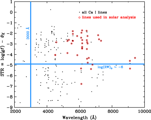
Figure 3. Relative strengths STR for the Ca i lines of this study. All lines with STR > −9 are shown with black circles, and those used in the solar abundance analysis are also circled in red. The 14 lines with STR < −9 not shown in this figure are too weak to be of interest in astronomical applications. The 3000 Å vertical line denotes the atmospheric wavelength cutoff for ground-based spectroscopy, and the horizontal line at STR ≈ −4.9 denotes the strengths of very weak solar lines, log(RW) ∼ −6 (EW = 5 mÅ at λ = 5000 Å).
Download figure:
Standard image High-resolution image5.1. Calcium in the Solar Photosphere
In most papers of this series some effort has been made to identify all appropriate transitions for a species in the solar photosphere. This is not necessary here, because all Ca i lines that are useful for abundance analysis have been cataloged previously. In Figure 3 we draw a horizontal blue line to denote the approximate STR level for photospheric lines that have very small equivalent widths (EWs). Using reduced widths log(RW) ≡ log(EW/λ) that are nearly wavelength independent, the line drawn at STR = −4.9 indicates the strength level for very weak lines on the linear part of the curve of growth, those with log(RW) ∼ −6.0 (equivalent to 5 mÅ at 5000 Å). Transitions with smaller strengths are difficult to identify with certainty and are subject to larger abundance uncertainties. The solar photospheric spectral line compendium by Moore et al. (1966), covering the optical spectral region (2935–8770 Å) lists ∼170 absorption features totally or partially attributable to Ca i. In Table 8, there are 87 lines with STR > −5.5 in the wavelength region 4000–8770 Å. Moore et al. identify 82 of these transitions in the solar spectrum, and all but one of the "missing" identifications are due to masking by very large transitions of other species. In the complex near-UV 3000–4000 Å region, 25 out of 30 lines with STR > −5.5 have solar identifications. Therefore, a search for useful Ca i transitions in the solar spectrum is unnecessary; that task was done by Moore et al.
Most of the solar Ca i lines in the yellow–red spectral region (λ > 5000 Å) have no substantial contaminants and as such can be treated to single-line EW analyses; detailed synthetic spectrum computations are not necessary. However, the majority of these lines are strong enough, log(RW) ≥ −5.0, to be saturated and thus be on the "flat" part of the curve of growth. This means decreased sensitivity of their EWs to abundance, with increased sensitivity to microturbulent velocity vt , and for the strongest lines some dependence on assumed damping parameters.
In Table 9 we list the EWs for the chosen Ca i lines. These were measured with SPECTRE 9 (Fitzpatrick & Sneden 1987), a specialized spectroscopic analysis code. The photospheric center-of-disk spectrum was the online BASS2000 version of Delbouille et al. (1973). 10 We matched the observed lines with Gaussian and/or Voigt model profiles along with direct integrations to derive the EWs.
Table 9. Ca i Equivalent Widths and Abundances
| λa | χa | log(gf) a | EW b | EW b | log εc | log εc |
|---|---|---|---|---|---|---|
| (Å) | (eV) | (mÅ) | (mÅ) | |||
| Sun | HD 84937 | Sun | HD 84937 | |||
| 2275.466 | 0.000 | −1.180 | ⋯ | ⋯ | ⋯ | 4.46 |
| 2398.559 | 0.000 | −1.360 | ⋯ | ⋯ | ⋯ | 4.41 |
| 3644.413 | 1.899 | −0.281 | ⋯ | 19.6 | ⋯ | 4.39 |
| 3875.776 | 2.526 | −0.842 | ⋯ | 4.0 | ⋯ | 4.56 |
| 4094.925 | 2.523 | −0.686 | ⋯ | 4.0 | ⋯ | 4.39 |
| 4226.728 | 0.000 | 0.239 | ⋯ | 153.0 | ⋯ | 4.48 |
| 4283.011 | 1.886 | −0.215 | ⋯ | 35.7 | ⋯ | 4.49 |
| 4289.367 | 1.879 | −0.310 | ⋯ | 29.5 | ⋯ | 4.45 |
| 4298.988 | 1.886 | −0.428 | ⋯ | 26.0 | ⋯ | 4.49 |
| 4302.528 | 1.899 | 0.267 | ⋯ | 60.0 | ⋯ | 4.48 |
| 4318.652 | 1.899 | −0.212 | ⋯ | 34.5 | ⋯ | 4.47 |
| 4355.079 | 2.709 | −0.426 | ⋯ | 4.9 | ⋯ | 4.37 |
| 4425.437 | 1.879 | −0.393 | ⋯ | 27.6 | ⋯ | 4.48 |
| 4434.957 | 1.886 | −0.040 | ⋯ | 44.3 | ⋯ | 4.46 |
| 4435.679 | 1.886 | −0.528 | ⋯ | 21.5 | ⋯ | 4.47 |
| 4454.779 | 1.899 | 0.228 | ⋯ | 59.5 | ⋯ | 4.47 |
| 4455.887 | 1.899 | −0.536 | ⋯ | 21.1 | ⋯ | 4.48 |
| 4456.616 | 1.899 | −1.723 | ⋯ | 2.1 | ⋯ | 4.57 |
| 4509.447 | 2.523 | −1.891 | 17.5 | ⋯ | 6.20 | ⋯ |
| 4512.268 | 2.526 | −1.900 | 23.2 | ⋯ | 6.40 | ⋯ |
| 4526.928 | 2.709 | −0.548 | ⋯ | 5.5 | ⋯ | 4.54 |
| 4578.551 | 2.521 | −0.697 | 80.7 | 4.5 | 6.28 | 4.43 |
| 4581.395 | 2.523 | −0.502 | ⋯ | 9.6 | ⋯ | 4.59 |
| 4585.866 | 2.526 | −0.338 | ⋯ | 11.0 | ⋯ | 4.49 |
| 5260.387 | 2.521 | −1.719 | 29.4 | ⋯ | 6.33 | ⋯ |
| 5261.704 | 2.521 | −0.579 | 95.0 | 6.7 | 6.42 | 4.47 |
| 5265.556 | 2.523 | −0.113 | ⋯ | 16.0 | ⋯ | 4.43 |
| 5349.465 | 2.709 | −0.310 | 98.3 | 8.3 | 6.27 | 4.47 |
| 5512.980 | 2.933 | −0.464 | 91.0 | 4.5 | 6.47 | 4.53 |
| 5581.965 | 2.523 | −0.555 | 92.0 | 7.5 | 6.31 | 4.49 |
| 5588.749 | 2.526 | 0.358 | 159.1 | 34.8 | 6.22 | 4.42 |
| 5590.114 | 2.521 | −0.571 | 89.7 | 6.8 | 6.29 | 4.46 |
| 5594.462 | 2.523 | 0.097 | 133.9 | 23.8 | 6.24 | 4.44 |
| 5598.480 | 2.521 | −0.087 | ⋯ | 18.0 | ⋯ | 4.46 |
| 5601.277 | 2.526 | −0.523 | ⋯ | 7.3 | ⋯ | 4.45 |
| 5857.451 | 2.933 | 0.240 | 146.0 | 17.0 | 6.39 | 4.46 |
| 5867.562 | 2.933 | −1.570 | 24.3 | ⋯ | 6.40 | ⋯ |
| 6097.266 | 2.521 | −3.177 | 2.3 | ⋯ | 6.48 | ⋯ |
| 6102.723 | 1.879 | −0.810 | 147.0 | 16.0 | 6.37 | 4.53 |
| 6122.217 | 1.886 | −0.339 | 214.0 | 33.5 | 6.33 | 4.49 |
| 6161.297 | 2.523 | −1.266 | 57.1 | ⋯ | 6.29 | ⋯ |
| 6162.173 | 1.899 | −0.116 | 270.0 | 44.5 | 6.37 | 4.48 |
| 6163.755 | 2.521 | −1.286 | 64.2 | ⋯ | 6.41 | ⋯ |
| 6166.439 | 2.521 | −1.142 | 72.0 | 2.2 | 6.39 | 4.50 |
| 6169.042 | 2.523 | −0.797 | 99.1 | 5.5 | 6.42 | 4.57 |
| 6169.563 | 2.526 | −0.478 | 116.8 | 8.4 | 6.31 | 4.46 |
| 6439.075 | 2.526 | 0.390 | 173.7 | 38.7 | 6.23 | 4.45 |
| 6449.808 | 2.521 | −0.502 | 101.5 | 10.0 | 6.32 | 4.55 |
| 6455.598 | 2.523 | −1.340 | 54.1 | ⋯ | 6.35 | ⋯ |
| 6462.567 | 2.523 | 0.262 | ⋯ | 31.3 | ⋯ | 4.42 |
| 6464.673 | 2.526 | −2.249 | 11.3 | ⋯ | 6.27 | ⋯ |
| 6471.662 | 2.526 | −0.686 | 93.5 | 5.9 | 6.39 | 4.49 |
| 6493.782 | 2.521 | −0.109 | 129.5 | 20.0 | 6.30 | 4.52 |
| 6499.650 | 2.523 | −0.818 | 88.4 | 5.7 | 6.42 | 4.60 |
| 6508.850 | 2.526 | −2.618 | 8.1 | ⋯ | 6.48 | ⋯ |
| 6572.779 | 0.000 | −4.320 | 26.8 | ⋯ | 6.38 | ⋯ |
| 6709.893 | 2.933 | −2.879 | 2.1 | ⋯ | 6.50 | ⋯ |
| 6717.681 | 2.709 | −0.524 | ⋯ | 6.4 | ⋯ | 4.52 |
| 6798.479 | 2.709 | −2.660 | 5.4 | ⋯ | 6.49 | ⋯ |
| 7148.150 | 2.709 | 0.137 | 152.1 | 22.5 | 6.33 | 4.49 |
| 7202.200 | 2.709 | −0.262 | 117.4 | 12.9 | 6.36 | 4.58 |
| 7326.146 | 2.933 | −0.208 | 115.0 | 9.0 | 6.44 | 4.55 |
| 9099.089 | 3.910 | −1.281 | 6.6 | ⋯ | 6.19 | ⋯ |
| 9108.827 | 3.910 | −2.005 | 1.2 | ⋯ | 6.15 | ⋯ |
| 9416.971 | 4.131 | −0.808 | 10.9 | ⋯ | 6.13 | ⋯ |
Notes.
a Ritz wavelengths and EPs and (recommended) log(gf) values are taken from Table 8. b Equivalent widths; typical uncertainties are ∼0.5 mÅ for the Sun and ∼1.0 mÅ for HD 84937. c log10 ε(X) = log10 (NX/NH) + 12; uncertainties from EW measurements are typically ±0.03 for individual lines; rising to ±0.04 for strong lines.We derived Ca abundances from these EWs with the LTE line analysis code MOOG (Sneden 1973).
11
The line parameters excitation energy and recommended log(gf) are given in Table 8. To ensure consistency with our previous studies of Fe-group and neutron-capture elements, we employed the older Holweger & Müller (1974) model photospheric atmosphere in the computations. The derived abundances in log ε units
12
are listed in Table 9 and plotted versus line wavelength in the top panel of Figure 4. From EW measurement uncertainties the abundance uncertainties are typically ±0.03 for individual lines. Total uncertainties depend on chosen solar photospheric model atmospheres, adopted line analysis codes, and radiative transfer assumptions. These are not explored in our work, which concentrates on Ca i transition probabilities. For a good discussion of modeling issues see Scott et al. (2015). The mean elemental abundance from 39 Ca i transitions is  = 6.34 ± 0.02 (σ = 0.09), as indicated in Figure 4. This value is in accord with other recent investigations of solar photospheric Ca abundance estimates: 6.34 ± 0.04 (Asplund et al. 2009) and 6.32 ± 0.03 (Scott et al. 2015).
13
Recommended meteoritic abundances are slightly lower: log ε = 6.31 ± 0.02 (Lodders et al. 2009), log ε = 6.27 ± 0.03 (Lodders 2020).
= 6.34 ± 0.02 (σ = 0.09), as indicated in Figure 4. This value is in accord with other recent investigations of solar photospheric Ca abundance estimates: 6.34 ± 0.04 (Asplund et al. 2009) and 6.32 ± 0.03 (Scott et al. 2015).
13
Recommended meteoritic abundances are slightly lower: log ε = 6.31 ± 0.02 (Lodders et al. 2009), log ε = 6.27 ± 0.03 (Lodders 2020).
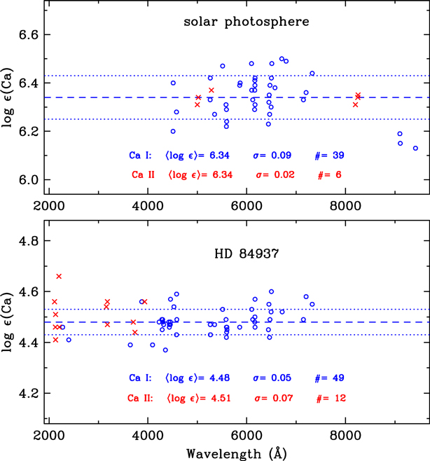
Figure 4. Line abundances for Ca i and Ca ii in the solar photosphere (top panel) and HD 84937 (bottom panel). The species are distinguished by blue colors for Ca i and red for Ca ii. In each panel horizontal lines are drawn to indicate the abundance mean and standard deviation σ derived for Ca i.
Download figure:
Standard image High-resolution imageWe also enlisted Ca ii to assist our solar Ca abundance determinations. Singly ionized Ca is a light (only slightly relativistic) atomic ion with one valence electron outside of closed shells. The relativistic calculation including single, double, and triple excitations of Dirac–Fock wave functions by Safronova & Safronova (2011) yielded transition probabilities for lines of Ca ii of high quality. Recently Kaur et al. (2021) tested the earlier work on Ca ii by Safronova & Safronova and expanded the earlier work to include lines of Mg ii, Sr ii, and Ba ii. Although the earlier work was motivated primarily by applications of Ca in atomic clocks, the excellent transition probabilities have important astrophysical applications. The transition probabilities by Kaur et al. (2021) agreed with those by Safronova & Safronova (2011) to well within 1% for nearly all lines.
Ca ii in the solar spectrum is dominated by Fraunhofer K (λ3933.7) and H (λ3968.5) and the near-IR triplet (λλ8498.0, 8542.1, and 8662.2) lines, but all of these features are extremely strong (log(RW) ≫ −4.0) and their line profiles are dominated by large damping wings. They are unreliable photospheric abundance indicators. However, Moore et al. (1966) identify nearly 20 other solar Ca ii transitions. The ones with λ > 4000 Å arise from lower transition levels that are high excitation (EP ≥ 6.5 eV). Our laboratory investigation did not include Ca ii, so we adopted transition probabilities from the theoretical computations of Safronova & Safronova (2011). The solar Ca ii lines are generally weak and/or blended, so we derived Ca abundances from synthetic/observed spectrum matches. In Figures 5(a)–(c) we illustrate these matches for three of the lines. The original Delbouille et al. (1973) photospheric spectrum has a wavelength step size of 0.002 Å, so for plotting clarity we have shown points separated by 0.016 Å.
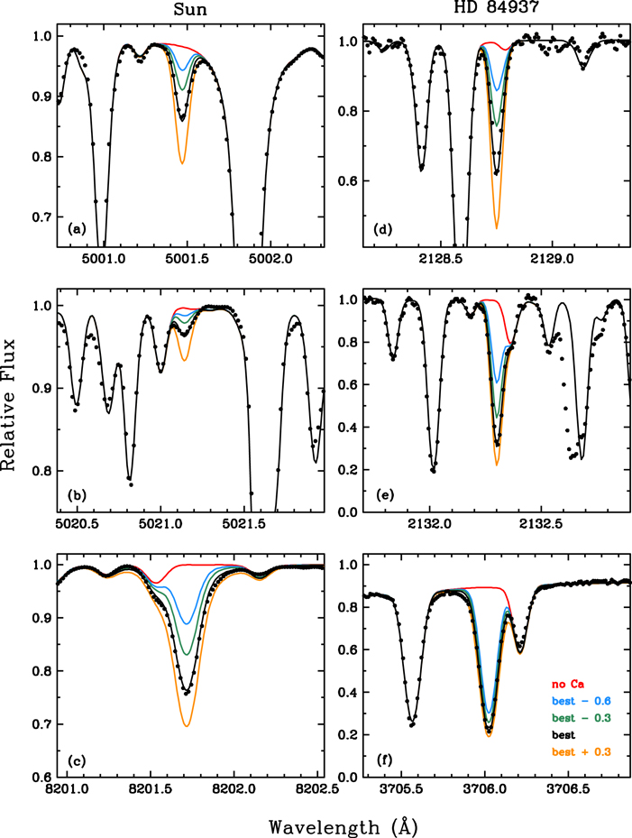
Figure 5. Observed and synthetic spectra of Ca ii lines in the solar photosphere (panels (a)–(c)) and HD 84937 (panels (d)–(f)). In each panel the observations are indicated with points and the synthetic spectra with lines colored to represent different logarithmic abundances of Ca. The black line in each panel is for the abundance that best matches the synthetic and observed spectrum for that Ca ii feature. Colors blue, green, and orange represent the best abundance offset by −0.6, −0.3, and +0.3 dex, respectively. The red line shows the effect of eliminating the Ca ii feature completely.
Download figure:
Standard image High-resolution imageTo construct the synthetic spectrum line lists, we employed the linemake facility (Placco et al. 2021), 14 which begins with the Kurucz (2011, 2018) 15 atomic line database and substitutes/modifies/adds atomic transition data from the papers published in this series and related studies by the Wisconsin lab atomic physics group, as well as molecular transition data from the Old Dominion lab molecular physics group (e.g., Brooke et al. 2016, and references therein). These line lists were used to generate initial synthetic spectra to be compared to the observations. The observed/synthetic matches were generally reasonable, but we then adjusted the line wavelengths and transition probabilities subject to the following restrictions. If a line has been reported in a study coauthored by the Wisconsin group, including the Ca i transitions reported here, its line parameters were accepted without change. The lines without such laboratory information were adjusted in wavelength and log(gf) to produce best matches to the observed spectra. In this way the excellent overall matches seen in Figure 5, and in Figure 6 to be discussed in Section 5.2, demonstrate that spectrum features surrounding the Ca features of interest have good identifications and can be used to accurately assess their contamination in crowded spectral regions. These good overall fits are not intended to yield reliable abundances for any features except those of Ca.
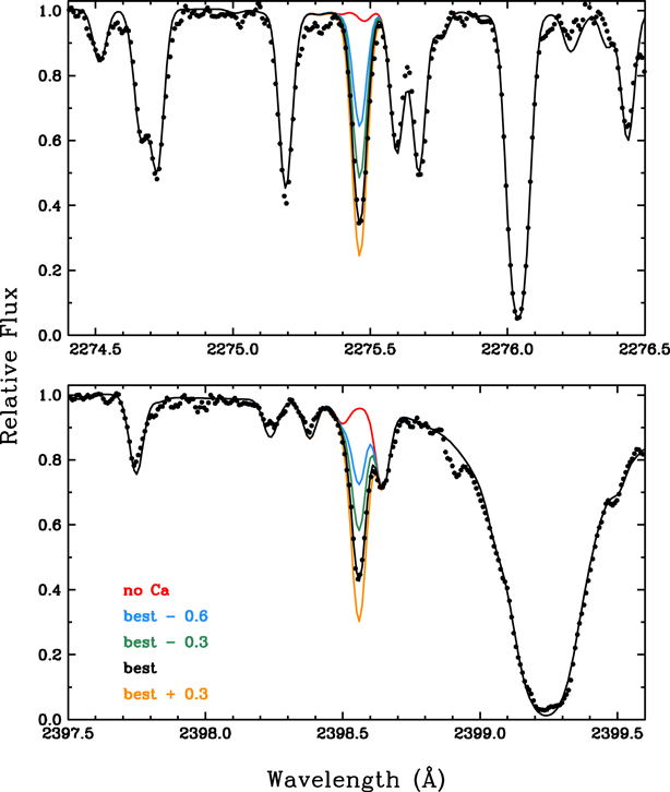
Figure 6. Observed and synthetic spectra of two ground-state (EP = 0.0 eV) transitions of Ca i in the UV spectrum of HD 84937. The symbols and colors are as in Figure 5.
Download figure:
Standard image High-resolution imageIn Table 10 we list the individual Ca ii solar line abundances. From six lines we derive elemental means  = 6.34 ± 0.01 (σ = 0.02), consistent within the uncertainties to that derived by Scott et al. (2015). The very small line-to-line scatter is probably a reflection of just the synthetic/observed spectrum fitting, because all six of the lines arise from the same lower energy level: 3p65p2P°. However, the agreement seen in Figure 4 between abundances derived for Ca i and Ca ii is encouraging. Most of Ca exists in its ionized species, due to the low first ionization energy: IP(Ca i) = 6.11 eV. A simple Saha ionization balance in line-forming regions of the solar atmosphere (τ ∼ 0.5) yields N(Ca ii)/N(Ca i) ∼ 103. On the other hand, the excitation energy of the Ca ii lines used for the solar analysis is high, EP = 7.51 eV, thus leading to significant temperature dependence of derived abundances. The excellent abundance agreement between neutral and ionized Ca species, combined with the similarity to previous photospheric and meteoritic results, suggests that the solar abundance derived with the new Ca i log(gf) values is reliable.
Table 10. Ca ii Abundances
| λa | χa | log(gf) | log ε | log ε |
|---|---|---|---|---|
| (Å) | (eV) | Sun | HD 84937 | |
| 2113.146 | 3.151 | −1.369 | ⋯ | 4.56 |
| 2128.750 | 1.692 | −3.319 | ⋯ | 4.46 |
| 2131.505 | 1.700 | −2.371 | ⋯ | 4.51 |
| 2132.304 | 1.692 | −2.658 | ⋯ | 4.41 |
| 2197.787 | 3.123 | −1.330 | ⋯ | 4.66 |
| 2208.611 | 3.151 | −1.027 | ⋯ | 4.46 |
| 3158.869 | 3.123 | 0.246 | ⋯ | 4.54 |
| 3179.331 | 3.151 | 0.504 | ⋯ | 4.56 |
| 3181.275 | 3.151 | −0.450 | ⋯ | 4.47 |
| 3706.024 | 3.123 | −0.453 | ⋯ | 4.48 |
| 3736.902 | 3.151 | −0.146 | ⋯ | 4.44 |
| 3933.663 | 0.000 | 0.113 | ⋯ | 4.56 |
| 5001.479 | 7.505 | −0.521 | 6.31 | ⋯ |
| 5021.138 | 7.515 | −1.222 | 6.34 | ⋯ |
| 5285.266 | 7.505 | −1.153 | 6.37 | ⋯ |
| 8201.72 | 7.505 | 0.318 | 6.31 | ⋯ |
| 8248.80 | 7.515 | 0.576 | 6.34 | ⋯ |
| 8254.72 | 7.515 | −0.378 | 6.35 | ⋯ |
Notes.
a Ritz wavelengths and excitation energies taken from the NIST ASD (Kramida et al. 2019). b log(gf) values are taken from the theoretical calculations of Theodosiou (1989) for the first four entries and from Safronova & Safronova (2011) for the remaining entries.Download table as: ASCIITypeset image
5.2. Calcium in HD 84937
As in our previous papers on Fe-group transitions (e.g., Den Hartog et al. 2019, and references therein), to test application of the new transition probability data to low-metallicity stars, we chose the main-sequence turnoff star HD 84937. The model parameters were those initially derived in Sneden et al. (2016): Teff = 6300 K, log g = 4.0, [Fe/H] = −2.15, and vt = 1.5 km s−1. The optical (ESO VLT UVES, Dekker et al. 2000; McDonald 2.7 m Tull Echelle, Tull et al. 1995) high-resolution spectra used here are discussed in detail in Sneden et al. The UV spectra were downloaded from the Mikulski Archive for Space Telescopes (MAST) and processed automatically by the CALSTIS pipeline. These spectra were obtained using the Space Telescope Imaging Spectrograph (STIS; Kimble et al. 1998; Woodgate et al. 1998) on board the Hubble Space Telescope, as part of program GO-14161 (PI Peterson). They cover 1879–3143 Å at a spectral resolving power of 114,000. Our abundance computations use the MOOG version that includes scattering in the continuum source functions (Sobeck et al. 2011), but in reality the scattering terms are not large even in the UV spectral domain of the warm, high-gravity HD 84937; H− remains the dominant continuum opacity source, followed by H i Balmer continuum opacity blueward of the Balmer jump (λ < 3646 Å).
Identification of useful Ca i lines was as straightforward as in the solar case described in Section 5.1. Nearly all of the transitions in Table 8 are in the optical domain, λ > 3250 Å, and all of the strong lines have solar identifications. The only UV transitions in this study are nine arising from the Ca i ground state.
We measured EWs and derived abundances as described in Section 5.1. These values are listed in Table 9 and plotted as a function of wavelength in the bottom panel of Figure 4. Additionally, we used synthetic spectrum computations to extract abundances from the ground-state lines in the UV. These transitions are important because most of the electrons in Ca i exist in the ground state instead of the excited states (whose minimum EP is 1.69 eV). There are three ground-state lines strong enough for detection in HD 84937: 2200.73, 2275.47, and 2398.56 Å. These transitions are indicated by blue lines in Figure 1 connecting to the 4s6p, 4snp, and 4s7p1P1 levels. Unfortunately, the λ2200.73 transition is completely masked by the very strong Fe i
λ2200.72 line, aided by a strong Ni i line at 2200.68 Å. In Figure 6 we show observed and synthetic spectra for the other two ground-state lines. The λ2275.47 line has only a very weak contaminant: Fe ii
λ2275.47, which gives rise to the ∼2% absorption seen at this wavelength in the no-Ca synthesis. The Fe ii transition is real, as it is listed in the NIST ASD (Kramida et al. 2019; the line is from an unpublished line list accompanying the lab study by Nave & Johansson 2013). However, no lab transition probability has been published, and the log(gf) value adopted for this line comes from the Kurucz database, one of the Fe ii lines with "semiempirical" computed values (e.g., Kurucz 1988, and references therein). The contamination of the Ca i line caused by this Fe ii line is probably very small, but it remains somewhat uncertain. Finally, the λ2398.56 transition, displayed in the bottom panel of Figure 6, is somewhat blended and must be analyzed via synthetic spectra. The HD 84937 mean abundance from the 49 Ca i lines is  = 4.48 ± 0.01 (σ = 0.05). The two UV ground-state lines, with
  = 4.44 (σ = 0.03 from the synthetic/observed spectrum fits), are in reasonable agreement with the overall average.
We derived abundance sensitivities to model atmosphere uncertainties in the manner computed by Sneden et al. (2016). In that paper, consideration of the many literature studies of HD 84937 suggested that parameter uncertainties are σ(Teff) ≈ ±80 K, σ(log g) ≈ ±0.15, σ([M/H]) ≈ ±0.15, and σ(vt ) ≈ ±0.1 km s−1. We altered the adopted HD 84937 model to assess the Ca i abundance changes in response to these parameter shifts. For temperature changes Δ(Teff) = ±150 K, Δ(log ε(Ca i)) ≈ ±0.07; for surface gravity changes Δ(log g) = ±0.25, Δ(log ε(Ca i)) ≈ ∓0.01; for metallicity changes Δ([M/H]) = ±0.25, Δ(log ε(Ca i)) < 0.01; and for microturbulent velocity changes Δ(vt ) = ±0.15 km s−1, Δ(log ε(Ca i)) ≈ ∓0.01. Clearly the greatest abundance sensitivity is to Teff. However, when these log ε are converted to [Ca/Fe] abundance ratios (Section 6), the similar sensitivities of Fe i to Teff uncertainties yield relatively small dependence of Ca i abundances on model parameters, as argued in Sneden et al. and other literature sources.
Many Ca ii lines are accessible in HD 84937. We show three examples of synthetic/observed spectrum matches in Figures 5(d)–(f). Although analyses of these lines are relatively straightforward, the spectrum of the λ2132.30 feature provides an illustration of the uncertainties of our procedure. The Ca ii line is primarily blended with Al i
λ2132.39. This contaminant is cataloged in the NIST ASD (from Penkin & Shabanova 1965) but without a transition probability, so our syntheses relied on a best empirical fit to set the Al i strength. Additionally, at about 2132.65 Å there is a missing transition in our synthetic spectrum line list. It does not have a plausible match in the Kurucz (2011, 2018) line compendium. The absence of a good match here serves as a cautionary note to our analyses: we cannot account for contaminants to the lines of interest if we have no empirical knowledge of their existence. With that caution in mind, it is clear that the 12 Ca ii lines yield internal agreement, leading to  = 4.51 ± 0.02 (σ = 0.07). This value agrees within mutual uncertainties with the mean abundance from Ca i.
Finally, repeating for Ca ii the parameter sensitivity computations, for temperature changes Δ(Teff) = ±150 K, Δ(log ε(Ca ii)) ≈ ±0.06; for surface gravity changes Δ(log g) = ±0.25, Δ(log ε(Ca ii)) ≈ ∓0.03; for metallicity changes Δ([M/H]) = ±0.25, Δ(log ε(Ca ii)) ≈ ∓0.02; and for microturbulent velocity changes Δ(vt ) = ±0.15 km s−1, Δ(log ε(Ca ii)) ≈ ∓0.06. The abundance shift with Teff change is largely driven by the sensitivity of H− continuous opacity to temperature in this H-R diagram domain, which affects also the Ca i abundance as discussed above. The relatively large sensitivity of log ε(Ca ii) to microturbulence is due to the large line strengths of the Ca ii lines used here.
5.3. Discussion
Utilizing our new Ca abundance determination and our previously derived Fe abundance for the well-studied halo star HD 84937 (Sneden et al. 2016), we derive a value of [Ca/Fe] = +0.46 for this star. Based on the discussion in the previous section regarding uncertainties in atmospheric parameters, we adopt a total error bar of ±0.07 in the log ε abundance of Ca. This error estimate does not include any possible NLTE effects for Ca or for Fe, but this may be an overestimate of the uncertainty in the ratio of [Ca/Fe] (see Sneden et al. 2016). We also look forward to determining this abundance ratio in additional stars with the same level of precision, utilizing the new experimentally determined atomic physics parameters. We compare this newly obtained value in Figure 7 with other low-metallicity halo stars from the survey of Roederer et al. (2014). That survey employed similar stellar parameters and model assumptions to our current calculations. It is clear from the figure that the abundance value for HD 84937 is entirely consistent with stars of similar metallicity in this survey. We have also made a similar abundance comparison with other data surveys that derived [Ca/Fe] (i.e., Cayrel et al. 2004; Barklem et al. 2005; Cohen et al. 2008; Lai et al. 2008; Yong et al. 2013) employing different stellar parameters than those of Roederer et al. (2014). Again, we find the newly derived abundance value of [Ca/Fe] for HD 84937 to be generally consistent with the measured values of stars of similar metallicity in these other stellar data surveys.
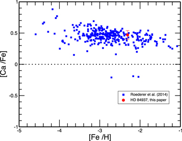
Figure 7. Calcium abundances [Ca/Fe] plotted vs. metallicity [Fe/H]. For plotting clarity we have chosen to compare our HD 84937 abundance to the general trend from one survey, Roederer et al. (2014).
Download figure:
Standard image High-resolution image
These types of abundance comparisons that illuminate Galactic chemical evolution serve as probes of star formation and nucleosynthesis over the history of the Galaxy (e.g., Kobayashi et al. 2020). For example, the abundance data shown in Figure 7 indicate that the [Ca/Fe] abundance ratios are relatively flat over most of the metallicity range studied, with a standard deviation in [Ca/Fe] of approximately ±0.08 for −3 < [Fe/H] < −2, which is within the range of measurement uncertainty. This consistency indicates a steady (and perhaps related) production mechanism for both Ca and Fe. Ca is produced in explosive burning in higher-mass stars, while Fe production comes from core-collapse supernovae early in the history of the Galaxy (e.g., Thielemann et al. 1996).
We note in the figure that at the lowest values of [Fe/H] there appears to be a slight rising trend in [Ca/Fe] with a fair amount of scatter, which may be related to differences in astrophysical or nucleosynthetic outcomes. Confirming whether and to what extent this trend is occurring is significant to understanding early Galactic nucleosynthesis and the (apparent) concomitant decrease in the formation of iron. It suggests that perhaps at some point the Ca and Fe production might be decoupled, possibly as a result of different stellar mass ranges or environments for the production of these two elements. Further, significant scatter at those very low metallicities might also suggest varying mass ranges for the first stars and/or inhomogeneity in early Galactic star-forming regions.
We also note that Type Ia supernovae contribute greatly to Fe production at higher metallicities and more recent epochs. The resulting downward trend of [Ca/Fe] as metallicities become larger (starting near [Fe/H] = −1) is evident in the figure. Clearly additional studies of Ca in the very lowest metallicity stars (less than −4), where there are little data, are warranted and would provide insight into the earliest production of these elements to address the question whether, for example, Ca production and Fe production differ greatly or are unrelated in the earliest, and presumably massive, stars.
We are endeavoring to obtain new Ca (and other elemental) abundance determinations for a range of metal-poor stars to help probe that early Galactic history (A. M. Boesgaard et al. 2021, in preparation). It will also be important to compare the Ca data with other α-element abundances, such as Si and Mg, to understand better the nature of both element production and star formation history at the earliest Galactic times.
6. Summary
The goals of this study have been to assemble the best experimental data—both new to this study and previously published—to test the reliability of modern theoretical transition probabilities for the light alkaline earth element Ca, and to assemble the most accurate and comprehensive line list of Ca i transition probabilities as is currently possible. We present new radiative lifetimes and BF (or BR) measurements for transitions of Ca i. These, combined with other quality experimental data are used to test the ab initio CI+MBPT calculations of M17. We find that for most transitions the calculations stand up well to the comparison, with the M17 log(gf) values falling within 0.2 dex of the experimental log(gf) values for all but six lines. We use a combination of the theoretical results augmented with experiment to produce a set of recommended log(gf) values for 202 transitions of Ca i ranging in wavelength from 2200 to 10000 Å. These data have been applied to the determination of the abundances of Ca in the Sun and the metal-poor star HD 84937.
This work is supported by NSF grants AST-1814512 (E.D.H. and J.E.L), AST-1616040 (C.S.), AST-1815403 (I.U.R.), and PHY 14-30152 (Physics Frontier Center/JINA-CEE) and NASA grants NNX16AE96G (J.E.L.), HST-GO-14765, and HST-GO-15657 (J.E.L. and I.U.R.). E.D.H. and J.E.L. would like to acknowledge the participation of Alex Scherer in the early stages of the radiative lifetime measurements.
Facilities: HST (STIS) - , VLT (UVES). -
Software: linemake (Placco et al. 2021), MOOG (Sneden 1973), SPECTRE (Fitzpatrick & Sneden 1987).
Footnotes
- *
Based on observations made with the NASA/ESA Hubble Space Telescope, obtained at the Space Telescope Science Institute, which is operated by the Association of Universities for Research in Astronomy, Inc., under NASA contract NAS 5-26555. The data presented in this paper were obtained from the Barbara A. Mikulski Archive for Space Telescopes. Other data have been obtained from the European Southern Observatory Science Archive Facility.
- 7
Formally an α-element is one whose dominant isotope is composed of multiple 4He nuclei. The major natural isotopes of Ca (Z = 20) are 40Ca (96.94% in the solar system), 42Ca (0.65%), 43Ca (0.14%), 44Ca, (2.09%), and 48Ca (0.19%); http://atom.kaeri.re.kr:81. For astrophysical purposes, Ca is pure 40Ca, making it the heaviest α-element in the periodic table. Since the minor isotopes of Ca collectively contribute only 3% to the Ca elemental abundance, they will be undetectable in solar and stellar optical spectra. Finally, note that the first spectrum of calcium (i.e., Ca i) refers to the spectrum of the neutral species.
- 8
The term "resonance line" refers to a transition that connects to the ground level.
- 9
- 10
- 11
- 12
We use standard abundance notations. For elements X and Y, the relative abundances are written [X/Y] = log10(NX/NY)star − log10(NX/NY)⊙. For element X, the "absolute" abundance is written log10 ε(X) = log10(NX/NH) + 12. Metallicity is defined as [Fe/H].
- 13
This is their best value after consideration of NLTE and 3D effects. These authors also computed an LTE abundance with the Holweger & Müller (1974) solar model, finding log ε(Ca) = 6.34.
- 14
- 15