


Abstract
THOR is the first open-source general circulation model (GCM) developed from scratch to study the atmospheres and climates of exoplanets, free from Earth- or solar-system-centric tunings. It solves the general nonhydrostatic Euler equations (instead of the primitive equations) on a sphere using the icosahedral grid. In the current study, we report major upgrades to THOR, building on the work of Mendonça et al. First, while the horizontally explicit and vertically implicit integration scheme is the same as that described in Mendonça et al., we provide a clearer description of the scheme and improve its implementation in the code. The differences in implementation between the hydrostatic shallow, quasi-hydrostatic deep, and nonhydrostatic deep treatments are fully detailed. Second, standard physics modules are added: two-stream, double-gray radiative transfer and dry convective adjustment. Third, THOR is tested on additional benchmarks: tidally locked Earth, deep hot Jupiter, acoustic wave, and gravity wave. Fourth, we report that differences between the hydrostatic and nonhydrostatic simulations are negligible in the Earth case but pronounced in the hot Jupiter case. Finally, the effects of the so-called "sponge layer," a form of drag implemented in most GCMs to provide numerical stability, are examined. Overall, these upgrades have improved the flexibility, user-friendliness, and stability of THOR.
Export citation and abstract BibTeX RIS

Original content from this work may be used under the terms of the Creative Commons Attribution 4.0 licence. Any further distribution of this work must maintain attribution to the author(s) and the title of the work, journal citation and DOI.
1. Introduction
1.1. The Atmospheric Circulation of Exoplanets
With new technology and data analysis techniques, we are entering an era in which 3D models of exoplanet atmospheres can be tested and validated. As observations improve, it will be important to test a variety of models, all of which make various assumptions in their representations of physical processes, to create the most accurate interpretations of the data.
Numerous theoretical and computational studies have shown that hot Jupiters have large day/night temperature contrasts and equatorial superrotation (Showman & Guillot 2002; Cooper & Showman 2005; Dobbs-Dixon & Lin 2008; Showman et al. 2009; Dobbs-Dixon et al. 2010; Rauscher & Menou 2010, 2012; Heng et al. 2011a, 2011b; Dobbs-Dixon & Agol 2013; Perez-Becker & Showman 2013; Kataria et al. 2015; Amundsen et al. 2016). These features are broadly consistent across a wide range of models and have been validated by observations (Snellen et al. 2010; Knutson et al. 2012; Louden & Wheatley 2015). The general consensus states that the superrotation is the product of interacting equatorial Rossby and Kelvin waves, which allow angular momentum to be transported toward the equator (Showman & Polvani 2011; Tsai et al. 2014; Hammond & Pierrehumbert 2018; Mendonça 2019).
Other works have explored the importance of clouds and hazes (Heng et al. 2012; Helling et al. 2016; Lee et al. 2016; Roman & Rauscher 2017; Mendonça et al. 2018a), atmospheric chemistry (Cooper & Showman 2006; Parmentier et al. 2013; Kataria et al. 2016; Drummond et al. 2018a, 2018b; Mendonça et al. 2018b), and shock physics (Goodman 2009; Li & Goodman 2010; Heng & Workman 2014; Fromang et al. 2016; Koll & Komacek 2018). Still others have focused on initial conditions and the details of numerical techniques (Thrastarson & Cho 2010, 2011; Watkins & Cho 2010; Liu & Showman 2013; Polichtchouk et al. 2014). These additional features are thought to be important, but the data are less conclusive in this regard (Heng & Showman 2015).
Further studies have focused on the atmospheric dynamics of other types of planets, including cooler Neptune-size planets (Charnay et al. 2015; May & Rauscher 2016; Mayne et al. 2019) and terrestrial planets (Merlis & Schneider 2010; Carone et al. 2014, 2016, 2018; Kaspi & Showman 2015; Guendelman & Kaspi 2018, 2019), particularly for the purposes of understanding habitability (Williams & Pollard 2002, 2003; Abe et al. 2011; Leconte et al. 2013a, 2013b; Yang et al. 2013, 2014; Kopparapu et al. 2016; Wolf et al. 2017; Way et al. 2018; Jansen et al. 2019). Atmospheric constraints for smaller and cooler planets, however, remain scarce because of the comparative difficulty of observation.
Even though constraining the atmospheric processes remains a challenge for extrasolar planets, the wide variety of orbits, masses, and sizes of planets indicates that the atmospheres will be quite diverse. Most studies of exoplanet atmospheres using general circulation models (GCMs) have adapted codes developed for Earth or solar system planets. The virtue of this method is that it relies on models that have been well tested; however, planet-specific tunings are often built into the code and can be difficult to find and generalize. In the development of THOR, we have chosen the opposite path: to develop a code from scratch that would be completely free of planet-specific tunings and would thus provide a flexible tool for the study of a diverse range of atmospheres. The additional benefit of this path is that we develop an intimate understanding of the physical processes at work and how these are represented in the code. The challenge that remains is the workload associated with development and testing new components.
Presented in Mendonça et al. (2016) and Mendonca et al. (2018) and utilized in Mendonça et al. (2018a, 2018b), THOR4 is a nonhydrostatic, fully global, 3D general circulation model developed specifically for the study of exoplanets. As such, it is free from the Earth and solar system tunings that often make use of 3D GCMs a challenge for exoplanets. However, because it is a young model developed from scratch, much development remains in order to make the model applicable to all types of planets. This work represents a step forward along this path.
The goals of this paper are to consolidate descriptions of improvements that have been made to the model since Mendonça et al. (2016), clarify the model framework, validate the new physics, and compare results from the model using different approximations, with implications for the general circulation of hot Jupiters.
2. Theory and Algorithm for the Dynamical Core
2.1. Preliminaries
The principal equations solved in THOR are the flux forms of the Euler equations:


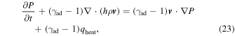
where ρ is the density, v is the velocity, P is the pressure, g is the acceleration due to gravity (assumed to be constant),  is the planet's rotation vector, and θ is the potential temperature. Potential temperature is defined as

The system of equations (Equations (1)–(3)) is closed by the ideal gas law, P = ρRdT. Additionally, a relationship between the pressure and potential temperature is necessary to update the pressure for use in Equation (2). From the ideal gas law and the definition of potential temperature, we have

THOR solves the Euler equations using a finite-volume method on an icosahedral grid (Tomita et al. 2001; Tomita & Satoh 2004; Mendonça et al. 2016). The horizontal resolution is controlled by a single parameter, glevel, the number of times the icosahedral grid is refined (i.e., the number of times the sides of the icosahedron are subdivided into smaller triangles). The average angular size of the control volumes is given by

The lowest value of glevel used in this work is 4, which results in an angular resolution of  . Every increase of glevel by 1 decreases
  by half. The average size (in m) of the control volumes is simply

where r0 is the planet radius. The value of  is used to scale the numerical diffusion coefficients (Section 2.4).
2.2. Discretizing the Equations
A full description of the THOR algorithm was presented in Mendonça et al. (2016); however, there were a number of typographical errors in that paper and some of the details have changed, so we include a description here.
As described in Mendonça et al. (2016), we use a time-splitting algorithm based on Wicker & Skamarock (2002), Tomita & Satoh (2004), and Skamarock & Klemp (2008). In this scheme, the fluid equations are split into fast and slow modes, and the fast modes are integrated using a smaller time step than the slow modes. The time-stepping loop consists then of an outer loop (the large time step, which has variable length) and an inner loop (small time step, with length designated Δτ).
During the inner loop (at time τ or τ + Δτ), the deviation of any quantity from its large time step value (at time t) is

or

where the  superscript indicates the deviation and the superscript in square brackets indicates how frequently the values are updated: slow modes (
![${}^{[t]}$](https://content.cld.iop.org/journals/0067-0049/248/2/30/revision1/apjsab930eieqn6.gif) ) are updated every large time step, and fast modes ([τ] or
) are updated every large time step, and fast modes ([τ] or ![${}^{[\tau +{\rm{\Delta }}\tau ]}$](https://content.cld.iop.org/journals/0067-0049/248/2/30/revision1/apjsab930eieqn7.gif) ) are updated every small time step. Broadly, the fast modes are those terms that are associated with acoustic waves, and the slow modes are everything else. This time-splitting method allows for a less stringent constraint on the time step and thus a moderate boost in performance, as many of the terms do not have to be computed as frequently (the advection terms are particularly costly). Further, the 3D operators are split into horizontal and vertical components (Mendonça et al. 2016)
) are updated every small time step. Broadly, the fast modes are those terms that are associated with acoustic waves, and the slow modes are everything else. This time-splitting method allows for a less stringent constraint on the time step and thus a moderate boost in performance, as many of the terms do not have to be computed as frequently (the advection terms are particularly costly). Further, the 3D operators are split into horizontal and vertical components (Mendonça et al. 2016)


The vector  represents the vertical direction, and r is the radial distance from the center of the planet. The altitude is given by z = r − r0.
Equations (1)–(3) are then discretized as
The terms  and
and  represent the horizontal and vertical components of the advection term,
  , and the terms
  and
and  represent the same for the Coriolis,
  . The terms
  ,
,  , and
, and  represent fluxes from the "slow" drag or numerical dissipation mechanisms, in this case, hyperdiffusion and Rayleigh friction. The additional term
  represents the 3D divergence damping, which needs to be evaluated on the small time step.
An important note regarding the coordinate system used in Equation (13): the 2D spherical surface represented by this equation is transformed into a 3D Cartesian coordinate system centered on the planet's core and rotating with the planet. For example, the horizontal velocity is defined as

where  represent the axes of this coordinate system and vi are the total (horizontal and vertical) velocities in the corresponding directions. The radial unit vector is related to the Cartesian coordinate system by

where ϕ is latitude and λ is longitude. In essence, Equation (16) defines the horizontal velocity as the total velocity minus the radial component. The advection and Coriolis terms,  and
and  , are defined in the same fashion. The use of a 3D Cartesian coordinate system allows the horizontal and vertical components of the advection and Coriolis terms (in Equation (2)) to be cleanly separated and is also used in the NICAM GCM (Tomita & Satoh 2004). The separation, in turn, is key to allowing explicit integration in time in the horizontal dimensions and implicit integration in the vertical dimension (see Section 2.3).
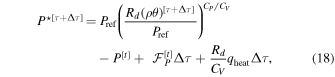
Our prognostic variables are ρ, P, ρvr, and the three Cartesian components of ρ vh, as well as their deviations. Despite using a thermodynamic equation for potential temperature, pressure is used as a prognostic rather than θ or ρθ. As noted in Mendonça et al. (2016), in THOR we do not calculate the deviation of ρθ from the large time step, because such calculation can lead to numerical instability. Instead, we calculate the new value, ![${\left(\rho \theta \right)}^{[\tau +{\rm{\Delta }}\tau ]}$](https://content.cld.iop.org/journals/0067-0049/248/2/30/revision1/apjsab930eieqn22.gif) , from Equation (15) and use this to update the pressure deviation, P⋆. Similarly, the dissipation and heating terms are applied to the pressure deviation, so that
, from Equation (15) and use this to update the pressure deviation, P⋆. Similarly, the dissipation and heating terms are applied to the pressure deviation, so that
where qheat represents all of the additional sources of heating or cooling (currently only radiation or Newtonian cooling).
Table 1 gives an overview of the variables used during integration of the dynamical core, the roles of each, and their properties. All quantities are defined at the horizontal centers of the control volumes, though there is some staggering of the grid in the vertical.
Table 1. Summary of Physical Quantities in Equations (12)–(18) and (35)–(36)
| Variable | Role | Location | Update |
|---|---|---|---|
| ρ | Prog. | Center | Large step |
| P | Prog. | Center | Large step |
| ρ vh | Prog. | Center | Large step |
| ρvr | Prog. | Midpoint | Large step |
| ρ⋆ | Prog. | Center | Small step |
| P⋆ | Prog. | Center | Small step |

|
Prog. | Center | Small step |

|
Prog. | Midpoint | Small step |
| θ | Diag. | Center | Large step |
| ρθ | Diag. | Center | Small step |

|
Diag. | Center | Large step |

|
Diag. | Center | Large step |

|
Diag. | Center | Large step |

|
Diag. | Center | Large step |
| h | Diag. | Center | Large step |

|
Diag. | Center | Large step |

|
Diag. | Center | Large step |

|
Diag. | Center | Large step |
| qheat | Diag. | Center | Master step |
Note. The "Role" column indicates whether the variable is a primary variable of the integration (prognostic) or a secondary variable (diagnostic). The "Location" column indicates whether variables are defined at the center of the vertical layers or the midpoint between two layers (though many quantities are interpolated to the midpoints to solve Equation (35)). The "Update" column indicates when each quantity is updated (Master step refers to an update outside the dynamical core loop; see Section 2.5).
Download table as: ASCIITypeset image
Table 2. Model Parameters for Newtonian Cooling Simulations
| Symbol | Description | Units | Synch. Earth | Deep Hot Jupiter |
|---|---|---|---|---|
| r0 | Planet radius | m | 6371,000 | 94,400,000 |
| g | Gravity | m s−2 | 9.8 | 9.42 |
| Ω | Rotation rate | rad s−1 | 1.996 × 10⁻⁷ | 2.06 × 10⁻⁵ |
| Rd | Gas constant | J K−1 kg−1 | 287 | 4593 |
| CP | Atmospheric heat capacity | J K−1 kg−1 | 1005 | 14308.4 |
| Pref | Reference pressure (bottom boundary) | bars | 1 | 220 |
| Tinit | Initial temperature of atmosphere | K | 300 | 1759 |
| ΔtM | Time step | s | 600 | 300 |
| ztop | Altitude of model top | m | 36000 | 8 × 10⁶ |
| glevel | Grid refinement level | ⋯ | 4/5 | 4 |
| vlevel | Number of vertical levels | ⋯ | 32 | 40 |
| Dhyp | Hyperdiffusion coefficient | ⋯ | 4.8 × 10⁻³ | 0.02 |
| Ddiv | Divergence damping coefficient | ⋯ | 4.8 × 10⁻³ | 0.03 |
| ksurf | Friction coefficient of lower boundary | s−1 | 1.1574 × 10⁻⁵ | ⋯ |
| σb | Boundary layer top (fraction of Pref) | ⋯ | 0.7 | ⋯ |
Download table as: ASCIITypeset image
Table 3. Model Parameters for Wave Simulations
| Symbol | Description | Units | Acoustic Waves | Gravity Waves |
|---|---|---|---|---|
| r0 | Planet radius | m | 6371,000 | 6371,000 |
| g | Gravity | m s−2 | 9.8 | 9.8 |
| Ω | Rotation rate | rad s−1 | 0 | 0 |
| Rd | Gas constant | J K−1 kg−1 | 287 | 287 |
| CP | Atmospheric heat capacity | J K−1 kg−1 | 1005 | 1005 |
| Pref | Reference pressure (bottom boundary) | bars | 1 | 1 |
| Tinit | Initial temperature of atmosphere | K | 300 | 300 (at Pref) |
| ΔtM | Time step | s | 1800 | 1800 |
| ztop | Altitude of model top | m | 10,000 | 10,000 |
| glevel | Grid refinement level | ⋯ | 5 | 5 |
| vlevel | Number of vertical levels | ⋯ | 20 | 20/40 |
| Dhyp | Hyperdiffusion coefficient | ⋯ | 0 | 0.01 |
| Ddiv | Divergence damping coefficient | ⋯ | 0/0.02 | 0.01 |
Download table as: ASCIITypeset image
Table 4. Model Parameters for Gray RT Simulations
| Symbol | Description | Units | Earth | HD 189733 b |
|---|---|---|---|---|
| r0 | Planet radius | m | 6371,000 | 79,698,540 |
| g | Gravity | m s−2 | 9.8 | 21.4 |
| Ω | Rotation rate | rad s−1 | 7.292 × 10⁻⁵ | 3.279 × 10⁻⁵ |
| Rd | Gas constant | J K−1 kg−1 | 287 | 3779 |
| CP | Atmospheric heat capacity | J K−1 kg−1 | 1005 | 13226.8 |
| Pref | Reference pressure (bottom boundary) | bars | 1 | 220 |
| Tinit | Initial temperature of atmosphere | K | 300 | 1600 |
| ΔtM | Time step | s | 500/300 | 150/100 |
| ztop | Altitude of model top | m | 36000 | 3.6 × 10⁶ |
| glevel | Grid refinement level | ⋯ | 5/6 | 4/5 |
| vlevel | Number of vertical levels | ⋯ | 32 | 40 |
| Dhyp | Hyperdiffusion coefficient | ⋯ | 4.8 × 10⁻³ | 9.97 × 10⁻³ |
| Ddiv | Divergence damping coefficient | ⋯ | 4.8 × 10⁻³ | 9.97 × 10⁻³ |
| S0 | Incident stellar flux | W m−2 | 1367 | 467072 |
| A0 | Albedo | ⋯ | 0.3135 | 0.18 |
| norb | Orbital mean motion | rad s−1 | 1.98 × 10⁻⁷ | 3.279 × 10⁻⁵ |
| nlw | Power-law index for long-wave optical depth | ⋯ | 4 | 2 |
| fl | Strength of well-mixed absorber (long-wave) | ⋯ | 0.1 | 0.5 |
| τlw,eq | Long-wave optical depth at Pref at equator | ⋯ | 6 | 4680 |
| τlw,pole | Long-wave optical depth at Pref at poles | ⋯ | 1.5 | 4680 |
| nsw | Power-law index for short-wave optical depth | ⋯ | 2 | 1 |
| τsw | Short-wave optical depth at Pref | ⋯ | 0.2 | 1170 |

|
Diffusivity factor | ⋯ | 1 | 2 |
| Csurf | Heat capacity of surface (lower boundary) | J K−1 m−2 | 107 | ⋯ |
| ksurf | Friction coefficient of lower boundary | s−1 | 1.1574 × 10⁻⁵ | ⋯ |
| σb | Boundary layer top (fraction of Pref) | ⋯ | 0.7 | ⋯ |
| ksp | Sponge layer strength | s−1 | ⋯ | 10−3 |
| ηsp | Bottom of sponge layer (fraction of ztop) | ⋯ | ⋯ | 0.8 |
| nlats | Number of latitude bins used in sponge layer | ⋯ | ⋯ | 20 |
Download table as: ASCIITypeset image
2.3. Solving the Vertical Momentum Equation
Rather than solving Equation (14) explicitly in time for the vertical momentum, ![${\left(\rho {v}_{r}\right)}^{\star [\tau +{\rm{\Delta }}\tau ]}$](https://content.cld.iop.org/journals/0067-0049/248/2/30/revision1/apjsab930eieqn33.gif) , we follow Tomita & Satoh (2004) in combining the continuity equation, vertical momentum equation, and thermodynamic equation to form a 1D Helmholtz equation that can be solved implicitly. The implicit solution has the advantage of stabilizing the model without having to resolve the timescale associated with vertically propagating acoustic waves. The resulting Helmholtz equation was presented in Mendonça et al. (2016); however, there were a number of typographical errors, and some steps of the derivation were not particularly clear. We take the opportunity to reproduce the full derivation and to correct the prior mistakes here. We must stress that the typos present in Mendonça et al. (2016) did not propagate to the code itself—in other words, the model was coded correctly, despite typos in the manuscript.
, we follow Tomita & Satoh (2004) in combining the continuity equation, vertical momentum equation, and thermodynamic equation to form a 1D Helmholtz equation that can be solved implicitly. The implicit solution has the advantage of stabilizing the model without having to resolve the timescale associated with vertically propagating acoustic waves. The resulting Helmholtz equation was presented in Mendonça et al. (2016); however, there were a number of typographical errors, and some steps of the derivation were not particularly clear. We take the opportunity to reproduce the full derivation and to correct the prior mistakes here. We must stress that the typos present in Mendonça et al. (2016) did not propagate to the code itself—in other words, the model was coded correctly, despite typos in the manuscript.
2.3.1. Preparing the Thermodynamic Equation
The use of the entropy equation, once discretized (Equation (15)), does not result in the Helmholtz equation presented in Mendonça et al. (2016) (Equation (37) in that paper). Rather, it is the energy form of the thermodynamic equation that is used (Equation (3) of Tomita & Satoh 2004):

where ρ is the density, e is the specific internal energy, h is the specific enthalpy, v is the velocity of the fluid, P is the pressure, and qheat is the diabatic heating rate. It can be shown that this equation is equivalent to Equation (3), aside from the heating term (see, e.g., Section 1.6 of Vallis 2006). However, once discretized, the discrete form for the pressure flux cannot be easily derived from the entropy version, so we begin here with the energy form. For reference, the specific internal energy and specific enthalpy are defined as


The internal energy can be written as Eint = ρe, which is also related to the pressure via the adiabatic gas index,  :
:

This allows us to write our thermodynamic equation as
or, since  ,
,

where Rd is the specific gas constant and CV is the heat capacity at constant volume.
Now, we designate "slow" and "fast" quantities and discretize as we did for Equations (12)–(15). Denoting the small time step τ and the large time step t, Equation (24) can be written as
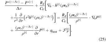
In this equation we also include the hyperdiffusive pressure flux, ![${{ \mathcal F }}_{P}^{[t]}$](https://content.cld.iop.org/journals/0067-0049/248/2/30/revision1/apjsab930eieqn36.gif) .
.
Using the fact that ![${\left(\rho {v}_{r}\right)}^{[\tau +{\rm{\Delta }}\tau ]}={\left(\rho {v}_{r}\right)}^{\star [\tau +{\rm{\Delta }}\tau ]}+{\left(\rho {v}_{r}\right)}^{[t]}$](https://content.cld.iop.org/journals/0067-0049/248/2/30/revision1/apjsab930eieqn37.gif) (from Equation (9)), Equation (25) becomes
(from Equation (9)), Equation (25) becomes
where we have collected horizontal velocity terms and large time step (t superscripted) terms on the right-hand side. Following Tomita & Satoh (2004), we evaluate the pressure gradient force (third term on the right-hand side) and the buoyancy force (fourth term on the right-hand side) at the large time step. This is not the optimal choice for the conservation of energy (Satoh 2013), but the resulting error is small compared to the errors introduced by the diffusion schemes, and it allows the resulting Helmholtz equation (Equation (35)) to be solved implicitly. To achieve a more concise form (and stay consistent in notation with Mendonça et al. 2016), we will introduce the effective gravity,

and define
Again, note that there are several typos in Equations (39) and (40) of Mendonça et al. (2016), which we have corrected in our Equations (27) and (28).
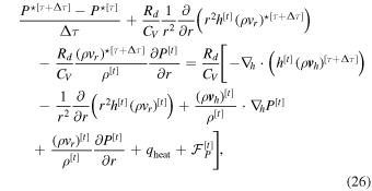
Then, Equation (26) becomes
Next, we must solve for ![${P}^{\star [\tau +{\rm{\Delta }}\tau ]}$](https://content.cld.iop.org/journals/0067-0049/248/2/30/revision1/apjsab930eieqn38.gif) and take its derivative in r to replace the pressure term in our vertical momentum equation. Noting that
and take its derivative in r to replace the pressure term in our vertical momentum equation. Noting that

and taking the derivative with respect to r, we have
The vertical derivative is taken here in order to eliminate the pressure at time [τ + Δτ] from the vertical momentum equation, as shown below.
2.3.2. Preparing the Continuity Equation
We begin with the discretized form of the continuity Equation (1) and define

which, like SP, incorporates the terms evaluated at the large time step and the horizontal momentum term (which is already evaluated for the current small time step).
To eliminate the density at time [τ + Δτ] from the vertical momentum equation, we simply solve for ρ⋆[τ+Δτ]:

2.3.3. Solving the Vertical Momentum Equation
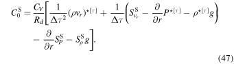
For the vertical momentum Equation (14), we again collect the terms evaluated at the large time step into a single term defined as

where  is the vertical component of the Coriolis acceleration and
  is the vertical component of the advection term
  . We now substitute Equations (31) and (33) into Equation (14) and arrange on the left-hand side all terms involving
 ![${\left(\rho {v}_{r}\right)}^{\star [\tau +{\rm{\Delta }}\tau ]}$](https://content.cld.iop.org/journals/0067-0049/248/2/30/revision1/apjsab930eieqn42.gif) (the deviation of the vertical momentum from the large time step [t] at time [τ + Δτ]). To achieve the final desired form, we divide through by ΔτRd/CV, resulting in
(the deviation of the vertical momentum from the large time step [t] at time [τ + Δτ]). To achieve the final desired form, we divide through by ΔτRd/CV, resulting in
where

Equation (35) is the final Helmholtz equation for the vertical momentum. Note that the version printed in Mendonça et al. (2016) contains several typos that have been corrected here.
2.3.4. The Hydrostatic and Shallow Approximations
The hydrostatic approximation that is commonly used in atmospheric models is derived by assuming that the vertical pressure gradient and gravitational force are much larger than the other terms in the vertical momentum equation, in other words,

Making this assumption results in the well-known equation for hydrostatic equilibrium:

In the work of Tomita & Satoh (2004), this assumption was made possible by maintaining a factor α next to all the terms in the vertical momentum equation except the two above (the pressure gradient and gravitational force), which could then be set to unity for nonhydrostatic or zero for hydrostatic, leaving the algorithm otherwise unchanged. This should be used with caution, however, as White et al. (2005) found that the application of hydrostatic balance solely to the vertical momentum equation produces an inconsistency in the representation of potential vorticity within the model unless the "shallow" approximation is also applied. Because of the mixture of coordinate systems in the Tomita & Satoh (2004) algorithm (Cartesian for the horizontal momentum and spherical for the vertical) and the form of the differential operators on the icosahedral grid, it is not simple to find exact correspondence between equations used in THOR and those studied in White et al. (2005). However, because the approximations discussed here refer implicitly to a spherical coordinate system, we believe that the problem described in that paper is relevant here. Hence, we follow their example in applying the hydrostatic and shallow approximations.
The first approximation, which we will call "quasi-hydrostatic" following the terminology used by White et al. (2005), involves neglecting the material derivative of the vertical velocity, in other words,

In practice, this involves not only the first term (the partial derivative in time) of Equation (14) but also the advection term,  . The method used to calculate
  in Cartesian coordinates from the vector momentum retains the effects of curvature (which result in the well-known "metric" terms in a fully spherical coordinate system); thus, we cannot merely discard
  from Equation (14). However, the metric part of
  can be simply calculated from the horizontal momentum, as

where vh is the horizontal momentum vector in Cartesian coordinates. Then, under the quasi-hydrostatic, deep (QHD) assumption, the vertical momentum equation becomes

As before, we use the thermodynamic and continuity equations to substitute the terms on the left-hand side, which results in the modified Helmholtz equation:
where
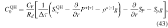
where  is computed using the QH version of the advection term,
  . Note that the hyperdiffusive flux term
  is also zero in this approximation. We then solve equations in the same fashion as in the nonhydrostatic model. Everywhere else, the equations remain identical to their nonhydrostatic versions.
The second approximation (the shallow approximation) is more involved. All horizontal differential operators are defined at the reference pressure (the bottom of the model), and these are proportional to 1/r0, where r0 is the radius of the planet (the distance from the center to the location of the reference pressure). To account for curvature, the horizontal operators are multiplied by r0/r, where r = r0 + z and z is the altitude. Simply, this scales the horizontal area of the control volumes with altitude. In the shallow approximation, r = r0, and the scaling is removed from the horizontal operators. The radial derivative in the divergence also changes, as follows:

where ψ is just a representative quantity. In this way, the second derivative (Equation (30)) becomes

Using this in the thermodynamic equation and again constructing the Helmholtz equation, we have
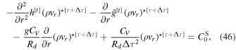
where
In this case,  ,
,  ,
,  , and all advection terms are calculated using the shallow operators described above. One additional change is made to ensure that the Coriolis acceleration is consistently represented by the horizontal and vertical equations. The Coriolis vector,
  , is now
where the unit vectors  represent the rotating Cartesian coordinate system fixed at the center of the planet (the spin axis is aligned with
  ), and the velocities vi are the total (horizontal plus vertical) in the corresponding direction. Equation (48) is equivalent to the form of Coriolis that appears in the primitive equations (i.e., the horizontal component of
  is neglected). The radial component,
  , is now equal to zero.
2.3.5. Discretizing and Solving the 1D Helmholtz Equation
The time-discretized 1D Helmholtz equation (Equation (35)) is now spatially discretized in the following way. The vertical momentum is solved for at the midpoints between layers, in contrast to the horizontal momentum, pressure, and density, which are solved for at the center of the layer. Denoting quantities defined at the center of layers with subscript c and quantities defined at the midpoint between layers (the interfaces) with subscript m, we write the first term in Equation (35) containing the second derivative in r as
for the ith midpoint (between layers), i.e., at  . Superscripts indicate the layer/midpoint at which each quantity is defined and are ordered such that the ith midpoint is at the bottom of the ith layer. Here,
 ![${h}_{m}^{i}={h}^{[t]}$](https://content.cld.iop.org/journals/0067-0049/248/2/30/revision1/apjsab930eieqn59.gif) and
and ![${W}_{m}^{i}={\left(\rho {v}_{r}\right)}^{\star [\tau +{\rm{\Delta }}\tau ]}$](https://content.cld.iop.org/journals/0067-0049/248/2/30/revision1/apjsab930eieqn60.gif) for the ith midpoint. For shorthand, the spatial separations are defined as
for the ith midpoint. For shorthand, the spatial separations are defined as
First derivatives are calculated by performing a first-order finite difference across the layers i and i − 1 and then interpolating to the midpoint. The resulting procedure, for terms 2–4 in Equation (35), is
where  represents the various arguments inside the derivatives for the ith midpoint.
The resulting spatially discretized equations for each midpoint i form a system of equations that can be written as

which we then solve using Thomas's algorithm for tridiagonal matrices and the boundary conditions  (n represents the index of the top layer). After applying the discretization process and rearranging terms, the resulting coefficients are
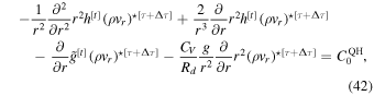
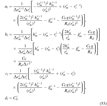
As before, the enthalpy is defined on the large time step at the ith midpoint, i.e., ![${h}_{m}^{i}={h}^{[t]}$](https://content.cld.iop.org/journals/0067-0049/248/2/30/revision1/apjsab930eieqn63.gif) , and likewise for
, and likewise for  and
and  .
.
Of course, in the case that the height grid is uniformly spaced,  and the above equations can be greatly simplified. The current version of THOR utilizes only a uniform grid; however, the model has been coded according to the above equations so that nonuniform grids can be utilized in the future. A further simplification can be made in the case of the shallow approximation, in which
  . This simplification is carried out in the model when the shallow approximation is used.
2.4. Numerical Dissipation
The flux-form hyperdiffusion terms that are applied to Equations (12)–(14) and (18) are


The divergence damping term in the horizontal momentum equation is

Note that the order of the gradient and Laplacian operators was incorrectly reversed in Mendonça et al. (2016); the model is coded as written in our Equation (58). Divergence damping is necessary to eliminate noise produced by the time-splitting integration scheme (Skamarock & Klemp 1992; Mendonça et al. 2016).
The diffusion coefficients, Khyp and Kdiv, have the same functional dependence on the grid resolution and time step size but can be individually adjusted. These are


where  is the average width of the control volumes given by Equation (7). The hyperdiffusion fluxes are updated on the large time step, while the divergence damping fluxes are updated every small time step.
The boundary conditions for the top and bottom of the model are that the vertical velocity must equal zero; this is the simplest assumption that allows for conservation of energy and axial angular momentum (Staniforth & Wood 2003). Unfortunately, this causes the boundary to act as a node for vertically propagating waves, causing them to reflect and potentially amplify. An additional dissipation mechanism is often needed to eliminate these reflecting waves. In a real atmosphere, vertical propagating waves will break in the upper layers; however, in the model the artificial reflection of these waves becomes an additional source of noise that can trigger numerical instabilities and cause the model to crash. Methods used to damp reflecting waves at the boundaries are often called "sponge layers." In THOR, we use the method based on Skamarock & Klemp (2008) and described in Mendonça et al. (2018b), which we briefly reiterate here.
The zonal, meridional, and vertical winds are all damped toward their zonal averages using Rayleigh friction. In principle, damping toward the zonal averages, rather than toward zero, will selectively damp waves while allowing the general flow to persist. In practice, the method is imperfect and the effect of the sponge layer on the flow at the highest layers is discernible as a decrease in the zonal wind speed. For this reason, we minimize the strength and size of the sponge layer in our simulations.
The damping takes the form

where v represents the vector velocity and  represents the zonal mean of the components, η = z/ztop is the fractional altitude, and ksp(η) is the damping strength as a function of the fractional altitude (with units of s−1).
The damping strength is a function of altitude and takes the form
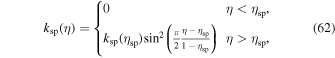
where ηsp, the fractional height at which the sponge layer begins, and ksp(ηsp) are values set by the user.
To calculate the zonal mean on our icosahedral grid, we divide the sphere into a user-set number of latitude bins, nlat, and compute the average within each bin. This is then considered as the average at the center latitude of each bin. At any given latitude, the zonal mean  is determined by linearly interpolating from the center of the respective latitude bin. This allows the zonal-mean velocities to vary more smoothly with latitude.
Equation (61) is calculated for the zonal, meridional, and vertical wind speeds. Since version 2.3 of the code, there are several options for the time integration of the sponge layer friction. In "implicit mode," which is used in the simulations here, the calculation of the rate of change in wind speed is done in the ProfX step (see Section 2.5), and the velocities are updated directly, implicitly, during this step. In "explicit mode," the rate of change is converted into fluxes that are passed to the dynamical core. For the vertical winds, this flux takes the form ρ dvr/dt (the vertical component of Equation (61)), which is added to Equation (56). For the horizontal winds, we first compute the zonal and meridional components of ρ dvh/dt, convert those to Cartesian coordinates, and then add them to Equation (55).
2.5. Time Integration
For clarity, we outline and summarize the flow of integration. At the top level, each time step contains two components: the dynamical core (THOR) and physics modules (ProfX); see Figure 1. The "dynamical core" refers to the solution of the Euler equations, and "physics modules" refers to any additional processes.
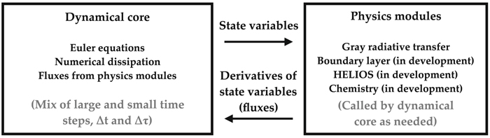
Figure 1. Top-level code structure of THOR. The dynamical core, which solves the Euler equations, passes state variables to the physics modules, which produces fluxes that are incorporated back into the dynamical core at designated code locations.
Download figure:
Standard image High-resolution image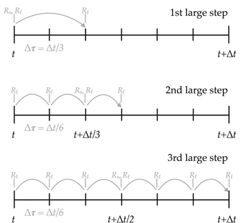
Figure 2. Schematic of the three large steps of the Runge–Kutta loop in THOR, for the example with the maximum number of small time steps nmax = 6. Rs and Rf represent the slow terms (superscript ![${}^{[t]}$](https://content.cld.iop.org/journals/0067-0049/248/2/30/revision1/apjsab930eieqn71.gif) ) and fast terms (superscripts
) and fast terms (superscripts ![${}^{[\tau ]}$](https://content.cld.iop.org/journals/0067-0049/248/2/30/revision1/apjsab930eieqn72.gif) and
and ![${}^{[\tau +{\rm{\Delta }}\tau ]}$](https://content.cld.iop.org/journals/0067-0049/248/2/30/revision1/apjsab930eieqn73.gif) ), respectively, and indicate when the terms are computed during each large step.
), respectively, and indicate when the terms are computed during each large step.
Download figure:
Standard image High-resolution imageThe integration of the dynamical core proceeds as follows. For any prognostic quantity, Φ, the value at time t + Δt is calculated using three large time steps of variable length (a third-order Runge–Kutta scheme; Wicker & Skamarock 2002; Tomita & Satoh 2004; Klemp et al. 2007; Mendonça et al. 2016). Each large time step is broken into smaller time steps of variable length: the first large time step consists of one small time step of length Δτ = Δt/3, the second large step consists of nmax/2 small steps of length Δτ = Δt/nmax, and the third large step consists of nmax steps of length Δτ = Δt/nmax.
A sketch of one time step for variable Φ follows, for nmax = 6 (see Figure 2). The beginning of the time step is time t. First, we calculate the slow terms in the derivative ∂Φ/∂t; these are the terms in Equations (12)–(15) and (18) designated with [t]. Next, we calculate the fast terms (designated with ![${}^{[\tau ]}$](https://content.cld.iop.org/journals/0067-0049/248/2/30/revision1/apjsab930eieqn74.gif) or
or ![${}^{[\tau +{\rm{\Delta }}\tau ]}$](https://content.cld.iop.org/journals/0067-0049/248/2/30/revision1/apjsab930eieqn75.gif) ) at times t and t + Δτ = t + Δt/3. The deviation, Φ⋆, is defined with respect to time t; thus, Φ⋆(t) = 0. The fast and slow terms are used to calculate Φ⋆(t + Δt/3), the deviation of Φ at time t + Δt/3. Then, we compute Φ(t + Δt/3) = Φ(t) + Φ⋆(t + Δt/3). This completes the first large step.
) at times t and t + Δτ = t + Δt/3. The deviation, Φ⋆, is defined with respect to time t; thus, Φ⋆(t) = 0. The fast and slow terms are used to calculate Φ⋆(t + Δt/3), the deviation of Φ at time t + Δt/3. Then, we compute Φ(t + Δt/3) = Φ(t) + Φ⋆(t + Δt/3). This completes the first large step.
The second large step begins. First, we recompute the deviations, which are now defined with respect to t + Δt/3, so that Φ⋆(t) = Φ(t) − Φ(t + Δt/3)  0. The slow terms (superscript
 ![${}^{[t]}$](https://content.cld.iop.org/journals/0067-0049/248/2/30/revision1/apjsab930eieqn77.gif) ) are recomputed at time t + Δt/3. The fast terms are recomputed at times t and t + Δτ = t + Δt/6 (again, nmax = 6 in this example). The fast terms at (t, t + Δt/6) and slow terms at t + Δt/3 are used to advance the deviations by a time step Δt/6, resulting in the value Φ⋆(t + Δt/6). Fast terms are recomputed at t + Δt/6 and t + 2Δt/6 = t + Δt/3, and these are used with the slow terms to advance one more step of size Δt/6, resulting in Φ⋆(t + Δt/3). We recompute the fast terms a third time and use them to compute Φ⋆(t + Δt/2), and finally Φ(t + Δt/2) = Φ(t) + Φ⋆(t + Δt/2). This completes the second large step.
) are recomputed at time t + Δt/3. The fast terms are recomputed at times t and t + Δτ = t + Δt/6 (again, nmax = 6 in this example). The fast terms at (t, t + Δt/6) and slow terms at t + Δt/3 are used to advance the deviations by a time step Δt/6, resulting in the value Φ⋆(t + Δt/6). Fast terms are recomputed at t + Δt/6 and t + 2Δt/6 = t + Δt/3, and these are used with the slow terms to advance one more step of size Δt/6, resulting in Φ⋆(t + Δt/3). We recompute the fast terms a third time and use them to compute Φ⋆(t + Δt/2), and finally Φ(t + Δt/2) = Φ(t) + Φ⋆(t + Δt/2). This completes the second large step.
The third large step begins. Again, the deviations are recalculated, this time with respect to t + Δt/2. Slow terms are recalculated at t + Δt/2, fast terms at t and t + Δt/6. These are used to calculate the deviation Φ⋆(t + Δt/6). The fast terms are then recomputed and the deviation updated for a total of nmax = 6 times. We then have Φ⋆(t + Δt), from which we calculate Φ(t + Δt) = Φ(t) + Φ⋆(t + Δt). This completes the Runge–Kutta loop.
A more detailed outline of a single time step is as follows:
- 1.ProfX step (additional physics)
- (a)Compute benchmark forcing if applicable. Typically, for benchmark tests, the prognostic variables are updated implicitly or explicitly during this step, rather than computing fluxes that are included in step 2.
- (b)Compute radiative transfer fluxes (Section 3.3). These are passed to the dynamical core as qheat, rather than updating thermodynamic variables directly during this step.
- (c)Update sponge layer quantities (zonal-mean winds and resulting drag, Equation (61)). These can be used to implicitly update the wind speed during this step (implicit mode) or passed as fluxes to the dynamical core and added to the hyperdiffusive terms
 and (explicit mode).
- 2.THOR step (dynamical core): solving fluid equations (Equations (12)–(15) and (18))
- (a)Begin large time step: three steps total, where the first step advances the prognostic variables to t + Δt/3, the second to t + Δt/2, and the third to t + Δt.
- i.Compute advection and Coriolis terms, , , at time t, t + Δt/3, or t + Δt/2 (for the first, second, and third steps).
- ii.
- iii.
- iv.
- v.Second and third large time steps only: update deviations ρ⋆,, , P⋆ (Equation (8)). Deviations are equal to zero on the first step.
- vi.Begin small time step: nstep steps, where nstep = (1, nmax/2, nmax) and Δτ = (Δt/3, Δt/nmax, Δt/nmax) for the first, second, and third large time step, respectively. For the nth iteration, the current time is τ = t + nΔτ.
- A.Update divergence damping (Equation (58)) at time τ.
- B.Compute horizontal momentum deviation (Equation (13)) at time τ + Δτ.
- C.
- D.
- E.Compute density deviations ρ⋆ (Equation (12)) at time τ + Δτ.
- F.Compute potential temperature density (ρθ) (Equation (15)) at time τ + Δτ.
- G.Compute pressure deviation P⋆ (Equation (18)) at time τ + Δτ.
- vii.End small time step.
- viii.Update prognostic variables ρ, (ρ vh), (ρvr), and P using final deviations from small time step loop. These are now defined at times t + Δt/3, t + Δt/2, or t + Δt, for the first, second, or third large step, respectively.
- (b)End large time step.


3. Added Physics
THOR's double-gray radiative transfer module is now publicly available. This module is based on Lacis & Oinas (1991) and Frierson et al. (2006). Details of the model are described in Mendonça et al. (2018a) and Section 3.3. Note that this version uses a two-stream flux formulation, wherein angle-integrated fluxes are calculated from the Stefan-Boltzmann law and the diffusivity factor is utilized to approximately capture the integral of intensity over angle. In Mendonça et al. (2018a), the integral of intensity over angle was performed using Gaussian quadrature; however, given the crudeness of the gray approximation, this angle integration is not strongly motivated, and a good choice of the diffusivity factor provides a solution that is accurate enough for our purposes. The double-gray RT code is placed into a modular structure so that it may be replaced by alternative forcing schemes (e.g., a more realistic radiative transfer model). Future versions of THOR will utilize the framework to couple to HELIOS (Malik et al. 2017).
Dry convective adjustment (Manabe et al. 1965; Hourdin et al. 1993) is now included in the public version of THOR, and we utilize it here in our simulations with radiative transfer. A mathematical description is given in Section 3.2.
Reproductions of the Held–Suarez test (Held & Suarez 1994) and the shallow hot Jupiter benchmark (Menou & Rauscher 2009; Heng et al. 2011b) using THOR were presented in Mendonça et al. (2016). Here we add to the list of benchmark tests the synchronously rotating Earth benchmark (Merlis & Schneider 2010; Heng et al. 2011b), the deep hot Jupiter benchmark (Cooper & Showman 2005, 2006; Rauscher & Menou 2010; Heng et al. 2011b), an acoustic wave test (Tomita & Satoh 2004), and a gravity wave test (Skamarock & Klemp 1994; Tomita & Satoh 2004). The code for all of the benchmark tests and the configuration files are included in the public repository.
3.1. Global Diagnostics
By default, the model now outputs additional diagnostic quantities: total energy, mass, angular momentum, and entropy. The mass, angular momentum, total energy (kinetic + internal + potential), and entropy of the ith grid point and jth vertical level are, respectively,
Above, ρ is the density, V is the volume of the control volume, r is the Cartesian vector position on the sphere,  is the vector rotation rate, vh is the horizontal wind vector, v is the total wind vector (horizontal + vertical), CV is the specific heat at constant volume, T is the temperature, g is the gravity (assumed to be constant), z is the altitude, CP is the specific heat at constant pressure, and θ is the potential temperature. Vectors are defined in a Cartesian coordinate system centered on the center of the planet and rotating about the
  -axis with rotation rate Ω. The vertical momentum can be ignored in the calculation of lij, as it is parallel to rij by definition. When integrated over the sphere, the nonaxial (
 and
and  ) components of the angular momentum should vanish; in practice, they are not identically zero because of numerical noise, so these components can provide a useful test of numerical accuracy.
The global total of each quantity is calculated by summing over i grid points and j vertical levels. In the deep model, the volume of the ith grid point and jth vertical level is

where Ai is the area of the ith control volume at the lowest boundary of the model, r0 is the planet radius, and  and
and  are the radial coordinates of the top and bottom boundaries of the jth layer. Figure 3 illustrates the calculation of the size of the control volume, Vij. The area, Ai, of each control volume is calculated during the grid construction (and adjusted by the spring dynamics process). This is calculated by decomposing the hexagon- or pentagon-shaped control volume into triangles formed by the center and two adjacent vertices (see Figure 2 of Mendonça et al. 2016) and summing the areas of the triangles. The areas of each triangle are calculated using the formula for spherical triangles
  , where the angles
  ,
,  , and
, and  are calculated from the vector locations of the center and corresponding vertices. When the shallow approximation is used, the control volumes are treated as flat, and so the volume is

Figure 3. Geometry of the control volumes. Left: top-down perspective of a hexagonal control volume (these can also be pentagonal). The total area is calculated by decomposing the volume into triangles, whose area can be found by the formula for spherical triangles and the angles  ,
,  , and
, and  , and then summing the areas of the six (or five, for pentagonal cells) triangles. Right: side profile of a control volume some distance rj above the surface. The total volume is found by integrating the area at the lower boundary,
  , to the upper boundary,
  .
.
Download figure:
Standard image High-resolution image3.2. Dry Convective Adjustment
Here we provide a description of the dry convective adjustment scheme, for completeness. Nonhydrostatic models require a parameterization for convection at the coarse resolutions we typically use for exoplanet modeling; typically, scales less than tens of kilometers must be resolved to capture convection with no parameterization in Earth simulations (Arakawa 2004; Jung & Arakawa 2004; Rio et al. 2019). This scheme is based on Hourdin et al. (1993). After the dynamical code time step, but prior to the calculation of radiative transfer/Newtonian cooling, each vertical column is searched for unstable layers. Static stability is given by the condition

where θ is the potential temperature. When an unstable layer is detected (meaning Equation (66) is violated), we define a "mixed" potential temperature, θmixed, equal to the average potential temperature in the layer. First, we integrate upward through the unstable layer to find the enthalpy h:

where P0, PB, and PT are the pressure at bottom of the entire column, the pressure at the bottom of the unstable layer, and the pressure at the top of the unstable layer, respectively. Then, the potential temperature across the entire layer is set equal to θmixed, given by
which is effectively like mixing the entropy across the unstable layer and enforcing an adiabatic profile in that region. After θmixed is calculated, the adjacent layers are tested for static stability again. If the adjacent layers are statically unstable with the new θmixed (e.g., the layer below, altitude-wise, has θ > θmixed), the entire process is repeated, including the additional unstable layers, until the entire column is statically stable.
3.3. Double-gray Radiative Transfer
The algorithm for radiative transfer is based on Lacis & Oinas (1991) and was described in Mendonça et al. (2018a). We do not reproduce the entire algorithm in this work, but we make several points of clarification.
We have reverted to using the diffusivity factor,  , instead of integrating intensities over angle using Gaussian quadrature as was done in Mendonça et al. (2018a). In the double-gray case, this approximation makes very little difference in the calculation of interlayer fluxes. When using multiwavelength radiative transfer, as in Lacis & Oinas (1991), more accurate integration over angle is probably warranted, but the double-gray approximation we use here is likely a much cruder assumption.
Our double-gray scheme is thus a true two-stream approximation, in which the diffusivity factor is used to calculate a characteristic angle for the path of the radiation, and radiation is assumed to be isotropic when the integral over angle is performed. In this approximation, the Planck functions in Equations (A1)–(A6) of Lacis & Oinas (1991) and Equations (3)–(8) of Mendonça et al. (2018a) are replaced by the angle-integrated flux calculated from the Stefan-Boltzmann law. The angle factor μ in those equations, as well as Equations (A9)–(A10) of Lacis & Oinas (1991) and Equations (9)–(10) of Mendonça et al. (2018a), is set to  , where
  is the diffusivity factor.
The optical depths are calculated using the form suggested by Frierson et al. (2006) and Heng et al. (2011a). For the short wave, we have a single power law:

where τsw,0 is the optical depth at P = Pref, σ = P/Pref, and nsw is a tuneable factor meant to control the vertical distribution of absorbers. For example, nsw = 1 would represent a uniformly mixed absorber. A value for nsw > 1 represents absorbers that are denser in the lower atmosphere.
The long-wave optical depth is given by

where τlw,w and τlw,s represent the surface optical depths of well-mixed absorbers and vertically segregated absorbers, respectively, and nlw is again a tuneable factor controlling the vertical distribution of the segregated absorbers. With a factor fl representing the percent of the surface optical depth attributable to the uniformly mixed absorbers, the optical depths above are given by

The surface optical depth τlw,0 can be assumed to be constant (hot Jupiter cases) or given a horizontal distribution. For our Earth-like double-gray case, we give τlw,0 a latitudinal dependence given by

where τlw,eq and τlw,pole are the surface optical depths at the equator and the poles, respectively. This latitudinal dependence approximates the effect of decreased water vapor concentration in the polar regions (Frierson et al. 2006).
The total fluxes passing through each layer are calculated from Equations (1)–(10) of Mendonça et al. (2018a). The heating in the nth layer, used in Equations (18) and (28), is
where  is the downward-propagating short-wave (stellar) flux,
  is the upward-propagating long-wave (thermal) flux,
  is the downward-propagating long-wave flux, and Δzn is the vertical thickness of the layer. Here qheat has units of W m−3, equivalent to kg m−1 s−3 or Pa s−1, in line with Equations (23) and (24).
As in Heng et al. (2011a), the surface (when used) is treated as a slab with a constant heat capacity, Csurf. The temperature is modeled using the relation

where  ,
,  , and
, and  are the short-wave and long-wave fluxes passing downward from and upward into the lowest atmospheric layer.
When no surface is included, as in our hot Jupiter simulations, the flux into and out of the lower boundary is zero, unless flux due to internal heating is included. We do not include flux from the interior in any of the simulations in this work; however, in the case where this is desired, it can be included by specifying an internal flux temperature, Tint.
The user can also set the planetary albedo, A0. In this double-gray scheme, the albedo represents a top-of-atmosphere albedo and is thus only applied as a modification of the incoming stellar flux, Q.
4. Further Benchmarks
4.1. Synchronously Rotating Earth
A benchmark test case for a synchronously rotating Earth using prescribed thermal forcing (Newtonian cooling) was suggested by Heng et al. (2011b) for comparison with the model of Merlis & Schneider (2010), which used gray radiative transfer. We repeat this test simulation here, with input parameters given in Table 2.
The temperature is forced toward an equilibrium profile given by

where
where ΔTEP is the temperature difference between the substellar and antistellar points (rather than the equator-to-pole difference), ΔTz is a characteristic scale for vertical temperature differences, and κad = Rd/CP is the adiabatic coefficient. This formulation is identical to the Held–Suarez test except for the second term of THS, which now depends on longitude, λ, to emulate the effect of having the substellar point permanently located at λ = 180° and ϕ = 0°. For the simulation here, ΔTEP = 60 K and ΔTz = 10 K, the same as in the Held–Suarez test. The damping timescale for temperature is also identical to the Held–Suarez test and is given by
where ka = 1/40 day−1, ks = 1/4 day−1, σ = P/Psurf, and σb = 0.7. The surface pressure, Psurf, is calculated at the lower boundary of the lowest layer.
The horizontal winds are damped toward zero with the timescale

where ksurf = 1 day−1.
Figure 4 shows results from the simulation with glevel = 5 (a horizontal resolution of ∼2°), plotted on two isobaric surfaces. Results are very similar for glevel = 4. At P = 0.9 bars, near the surface, we see convergence toward the substellar point (located at longitude λ = 180°), associated with the rising motion due to the intense heating at this location. At P = 0.25 bars, the flow diverges from the substellar point and then converges on the night side of the planet.
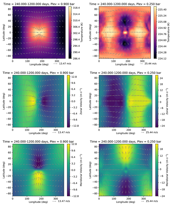
Figure 4. Output from the synchronously rotating Earth benchmark, temporally averaged from 240 to 1200 days. In color, the top panels show the temperature, the middle panels show the zonal wind speed, and the bottom panels show the meridional wind speed. The total horizontal winds are overplotted as arrows. The left column corresponds to a pressure level of 0.9 bars, the right to 0.25 bars.
Download figure:
Standard image High-resolution imageFigure 5 shows several properties as a function of latitude. On the night side, the temperature is highest at P ∼ 0.8 bars, well above the surface. On the day side, the temperature is highest at the equatorial surface. The transport of heat upward and away from the substellar point is apparent from the temperature distribution centered on λ = 180° and the stream function, which shows a large equator-to-pole Hadley cell in each hemisphere. The potential temperature distribution shows that the atmosphere is marginally unstable near the substellar point. Convective adjustment was not included here.
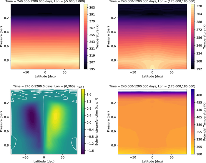
Figure 5. Additional quantities from the synchronously rotating Earth benchmark, viewed as a function of latitude and pressure level. The top left panel is the temperature averaged over a 10° slice over the antistellar point; the top right is the temperature averaged over a 10° slice over the substellar point; the bottom left is the Eulerian mean stream function (positive values indicate clockwise motion); the bottom right is the potential temperature averaged over 10° over the substellar point. In the plot for potential temperature, a narrow region near the top is masked to allow the structure in the lower atmosphere to be discernible—the potential temperature increases sharply up to ∼1000 K in the masked region. As in Figure 4, values are averaged over the interval of 240–1200 days.
Download figure:
Standard image High-resolution imageFor this test, we have not included heating and cooling of the surface. The pressure in the lowest atmospheric layer varies from ∼0.93 bars near the antistellar point to ∼0.91 bars near the substellar point. Extrapolating the atmospheric temperature to the reference pressure (roughly the location of the implied surface) for plotting purposes produces poor results because of the steep gradients at the bottom of the model that are not well resolved by our uniform vertical mesh; hence, we do not attempt to extend our figures to this region.
In general, the results compare well with Heng et al. (2011b) and Merlis & Schneider (2010). The temperatures and wind speeds are similar to those of Heng et al. (2011b), with a temperature peak at ∼320 K at the equator, near the surface, and max wind speeds of ∼13 m s−1 and ∼25 m s−1 at P = 0.9 and P = 0.25 bars, respectively. The fact that the nightside temperature in Figure 4 is warmer than that which appears in Figure 3 of Heng et al. (2011b) is due to the difference in pressure level, owing to the poor vertical resolution near the surface in our simulation. The temperatures are ∼20 K lower across the globe in the simulation of Merlis & Schneider (2010), which utilized a radiative transfer scheme; the fact that our temperatures agree with those in Heng et al. (2011b) suggests that this is due to the tuning of the temperature forcing in Equations (75) and (76) rather than an error in the code. The temperature distribution is otherwise similar to Figure 9 in Merlis & Schneider (2010), with a maximum near 0.8 bars on the night side. The Hadley cells are similar in size to theirs, though it is about a factor of 2 weaker in our simulation.
4.2. Deep Hot Jupiter
Here we attempt to reproduce the deep hot Jupiter benchmark test from Heng et al. (2011b). Input parameters are given in Table 2. Like the Held–Suarez test, the benchmark is run with an idealized forcing to the temperature (the winds, in this case, are unforced). As noted in Mayne et al. (2014), this benchmark has several challenges. First, in a nonhydrostatic model, where the vertical coordinate is altitude rather than pressure, the night side of the planet tends to extend to several orders of magnitude lower pressure than the day side. The exact temperature–pressure profiles suggested by Heng et al. (2011b) tend to lead to runaway cooling on the night side at the start of the simulation, causing the model to crash. Mayne et al. (2014) successfully mitigated this issue in the UK Met Office model by increasing the temperatures at low pressures. We have attempted the same here, with less success. The second issue is the discontinuity in the temperature–pressure profiles at 10 bars, which can lead to numerical instabilities. To avoid the issue, we refit the temperature–pressure profiles used in Heng et al. (2011b) with a new set of polynomials, excluding the pressures near 10 bars. This produces a new profile that varies smoothly in this region. The new polynomial fits are shown in Figure 6 and presented in Appendix A.
Figure 7 shows the zonal-mean temperature and zonal wind for the resulting simulation. Unfortunately, our model domain is limited to pressures ≳10 mbar on the day side of the planet. Raising the model top any further causes the nightside instability (noted by Mayne et al. 2014 and described above) to occur. At present, it is unclear why the UK Met Office model is able to successfully extend the model domain to lower pressures while THOR is not. However, based on the issues discussed here and in Mayne et al. (2014), it appears that the deep hot Jupiter benchmark is a challenge to reproduce in altitude-grid models.
We have made several attempts to extend the model domain, including initializing the atmosphere from the average Teq (blue curve in Figure 6) rather than isothermal conditions, including a sponge layer (see Section 2.4) at the top of the model, tuning the strength of divergence damping and hyperdiffusion, and initializing with a zonal wind profile to prompt dayside-nightside mixing. None of the above efforts were successful at preventing the runaway cooling on the night side that leads to a model instability.
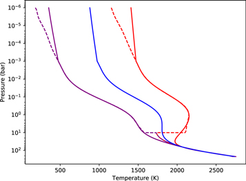
Figure 6. Temperature–pressure profiles used in the deep hot Jupiter benchmark test. The equilibrium temperature is equal to Tday (red) at the substellar point and equal to Tnight (purple) at the antistellar point. For each location on the planet, the equilibrium temperature is interpolated between Tday and Tnight based on the latitude and longitude. Dashed curves are the original profiles from Heng et al. (2011b); solid curves are the profiles used in this work. The blue curve represents the average.
Download figure:
Standard image High-resolution image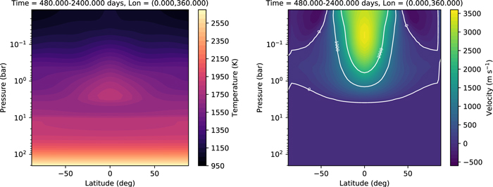
Figure 7. Zonally and temporally averaged temperature (left) and zonal wind speed (right) in the deep hot Jupiter simulation. The time average was performed over days 480–2400 of the simulation. The top altitude is limited to pressures of ∼10−2 bars at the hottest location on the planet.
Download figure:
Standard image High-resolution imageEven with the model domain limited to P ≳ 10 mbar on the day side, we do reproduce many of the features of the experiment done in previous works. We see a zonal-mean temperature that is similar in magnitude and structure to that of Heng et al. (2011b) and Mayne et al. (2014). We see equatorial superrotation and return flow at the midlatitudes. The jet speed we find here is weaker (∼3600 m s−1) than in the finite-volume simulation of Heng et al. (2011b; ∼5000 m s−1) and the simulation in Mayne et al. (2014; ∼6000 m s−1). This may be caused by the lower location of the model top (the velocities tend to increase with altitude), though it is also possibly explained by the low horizontal resolution we used for the simulation here (we revisit the problem of resolution in Section 5).
4.3. Acoustic Wave Experiment
Here we demonstrate the THOR GCM's representation of acoustic waves. The purpose of this test is to characterize how well the model is able to represent the propagation of acoustic waves and provide a tool to isolate coding errors that may be hard to diagnose in more complicated scenarios. The setup is almost identical to Section 4.1 of Tomita & Satoh (2004), but we describe it here for completeness. The atmosphere is initialized with a background isothermal state, for an Earth-radius planet with no rotation and no forcing (radiation or Newtonian cooling). At the beginning of the first time step, a pressure perturbation is applied over a spatial distribution centered on longitude λ0 = 0° and latitude ϕ0 = 0°. The distribution in latitude ϕ and longitude λ is given by

where L is a representative horizontal length and x is the horizontal distance along a great circle from the point (λ0, ϕ0) and is given by

The vertical distribution is

where z is the altitude, ztop is the height of the model top, and nv is the vertical wave mode. The total initial perturbation field is

where δp is the amplitude of the perturbation. Here, as in Tomita & Satoh (2004), we set δp = 100 Pa, r0 = 6371 km, L = r0/3, nv = 1, and ztop = 10 km. Further input parameters are given in Table 3.
We compare results from two simulations. In the first, both hyperdiffusion and divergence damping are omitted (by "divergence damping" we are referring to the terms that depend on the divergence of momentum in Equations (44)–(46) of Mendonça et al. 2016, Equation (58) in this work). In the second, only divergence damping is enabled, with a coefficient Ddiv = 0.02 (hyperdiffusion is still disabled). In Figure 8, we show the resulting pressure field in the lowest altitude level at different times for the case with divergence damping. These compare well with Figure 3 of Tomita & Satoh (2004). We note, however, that the amplitude of the pressure perturbation in their figure appears much larger than in ours, peaking at p' ≈ 1000 Pa, which seems inconsistent with an initial perturbation of δp = 100 Pa as stated in the text. We also see that the amplitude decreases as the wave spreads away from the point of origin (evident in the ranges of the color scales in Figure 8), which is not seen in the Tomita & Satoh (2004) figure, unless their color scale is mislabeled.
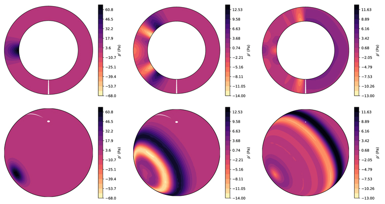
Figure 8. Density perturbation in the acoustic wave experiment. The top panels show the vertical profile around the planet along longitudes 0° and 180°. The bottom panels show the lowest horizontal level (altitude 250 m). The columns correspond to times t = (0, 4, 8) hr, from left to right. The plot style and perspective are chosen to facilitate direct comparison with Tomita & Satoh (2004). The density perturbation begins at (λ, ϕ) = (0°, 0°) and propagates around the planet, reaching the opposite side of the planet in ∼17 hr.
Download figure:
Standard image High-resolution imageIn Figure 9, we plot the globally integrated total energy, internal plus potential energy, and kinetic energy as a function of time. Compare with Figure 4 of Tomita & Satoh (2004)—though note that their figure has different units. There appears to be a slight mismatch between the exact hydrostatic initial conditions and the THOR algorithm's representation of hydrostatic balance. This leads to a jump in the total energy (on the order of 1014 J) on the first time step as all columns of the atmosphere adjust very slightly. At present the origin of the discrepancy is unclear, but in any case, the error is quite small compared to the total energy of the atmosphere and should not noticeably affect the results of simulations that include forcing, which produces a much larger change in the overall energy budget compared to the initial conditions. The pressure perturbation is applied at the end of the first time step, reaches the opposite side of the planet in ≈17 hr, and returns to the original location in ≈33 hr, indicating a sound speed of ∼337 m s−1, as found in Tomita & Satoh (2004). The theoretical sound speed is  m s−1, where γ = CP/CV.
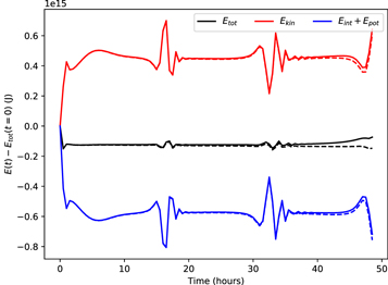
Figure 9. Total, internal plus potential, and kinetic energy in the acoustic wave experiment, as a function of time. Solid curves are for the simulation with no dissipation; dashed curves are for the simulation with divergence damping. There is some slight adjustment to hydrostatic equilibrium at the beginning of the simulation that results in temperature changes of <0.1 K everywhere, and small variations in the energies when the waves meet at ∼17 and ∼34 hr. The simulation with no damping has a large energy error that begins to accumulate rapidly after 40 hr and ultimately crashes the model. With divergence damping enabled, there is a small amount of energy loss. The changes in energy (∼1014 J) are quite small compared to the total energy of the atmosphere (1024 J).
Download figure:
Standard image High-resolution imageFrom Figure 9, we can see that the variation of kinetic energy associated with the sound wave is well compensated by the variation in internal plus potential energy. In the case without divergence damping, the total energy begins to increase erroneously after ∼35 hr. The simulation crashes not long after this time. This is the result of grid-scale noise that would be well eliminated by the divergence damping terms. A comparison between the damped and undamped cases of the global pressure field at 48.5 hr is shown in Figure 10. In the undamped case, we see spurious waves originating from the pentagonal grid points, but these waves are fully eliminated in the damped case.
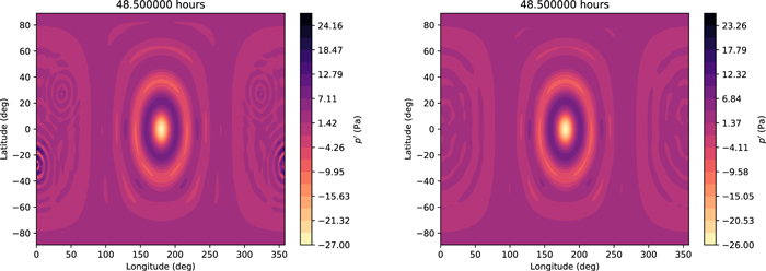
Figure 10. Comparison of pressure field for the acoustic wave simulation at z = 250 m with no damping (left) and with divergence damping (right).
Download figure:
Standard image High-resolution imageThe case with divergence damping conserves the energy much better, though there is a slight energy loss over the course of the simulation. Comparing with Tomita & Satoh (2004), THOR does not conserve energy as well as their model NICAM. Our choice of entropy as the fundamental quantity in the thermodynamic equation rather than total energy means that the total energy is not conserved as precisely (Satoh 2002, 2003). Mendonça et al. (2016) tested an energy correction scheme in THOR based on Williamson et al. (2009) that, while improving total energy conservation, had little impact on the overall behavior of the model. Thus, until we can develop a more robust general approach that is physically well described at coarse resolutions, we choose to live with the gradual loss of energy to the dissipation scheme.
4.4. Gravity Wave Experiment
A further benchmark compares the representation of gravity waves in THOR with NICAM. The motivation behind this type of simulation is to characterize the model's representation of gravity waves. This test is originally presented in Tomita & Satoh (2004). We set up the atmosphere in the same manner as in that paper and in the acoustic wave experiment of the previous section, using the same planet radius, model top, and shape of the perturbation. See Table 3 for the input parameters. The key differences between these simulations and that in Section 4.3 are that the atmosphere is given a thermal profile corresponding to a constant Brunt–Väisälä frequency, instead of an isothermal profile, and the perturbation is applied to the potential temperature, given by

where θ' is the potential temperature perturbation function and δθ is its amplitude. The horizontal and vertical distributions, ξ and ζ, are again given by Equations (79) and (81). In all cases, δθ = 10 K.
The atmosphere for this case is initialized with a constant Brunt–Väisälä frequency, N. This can be defined in terms of the potential temperature as

In order to reduce numerical instabilities and to minimize motion introduced by the initial conditions, we initialize the atmosphere from hydrostatic equilibrium. For an atmosphere with a constant N, we must numerically solve the hydrostatic equation for the pressure of each layer as a function of the layer below. In our case, we begin at the reference pressure Pref, which is the pressure at the bottom of the lowest layer at the beginning of the simulation. From there, we progress upward, numerically determining the pressure of each successive layer. More specifically, we use Newton–Raphson iteration to find the pressure in the ith layer that satisfies the equation

The relationship between the pressure and density is given by the ideal gas law. An additional constraint must then be made on the temperature, which can be derived from the definition of N:

where

The quantities Pi−1, ρi−1, and Ti−1 are the pressure, density, and temperature of the layer below the ith, except in the case of the lowest layer, where Pi−1 = Pref,  , and Ti−1 = Tinit. Tinit is a user-set initial reference temperature. The value of Δz is the distance between the centers of the layers except in the case of the lowest layer, where it is simply the height of the lowest layer. After making the initial guess that ρi = ρi−1, we do one Newton–Raphson step to find a new value of Pi, update Ti and ρi (via Equation (86)), and then repeat the process until the change in Pi is below some threshold (we use 10−8).
In Figure 11, we show the results of three simulations. The first has (N, nv) = (0.01 s−1, 1), the second (N, nv) = (0.02 s−1, 1), and the third (N, nv) = (0.01 s−1, 2). The number of vertical levels is 20 in the nv = 1 cases and 40 in the nv = 2 case. The color contours show the temperature perturbation, ΔT, at the equator after 48 hr of integration. Tomita & Satoh (2004) give a theoretical estimate for the gravity wave speed, cg = Nztop/πnv, which is 31.8, 63.7, and 15.9 m s−1 in the three respective cases. The leading peaks in the three cases are located at λ ≈ (55°, 95°, 30°), indicating speeds cg ≈ (35, 61, 19) m s−1. Tomita & Satoh (2004) noted, in particular, the larger relative error in their nv = 2 case (cg ≈ 18 m s−1) and theorized that this was caused by insufficient vertical resolution—they used 20 vertical levels in this case. However, we have run the same test with 20 levels and 40 levels (the bottom panel of Figure 11 shows the 40 level case), and the locations of the wave peaks are virtually identical in both cases. Most likely, the error in the speed is dominated simply by the difficulty in estimating the locations of the wave fronts.
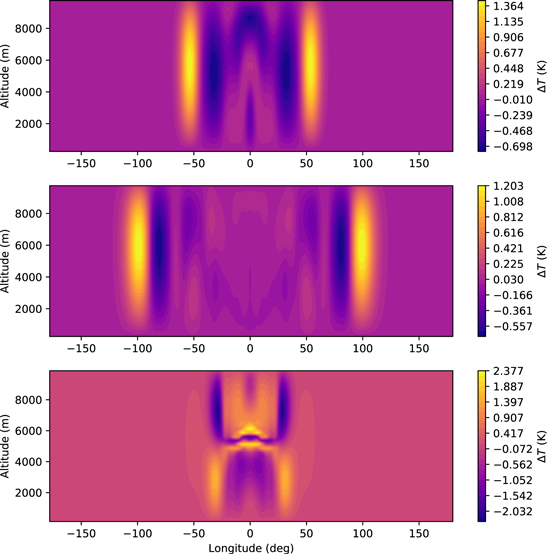
Figure 11. Temperature perturbation along the equator in the gravity wave simulations at 48 hr. ΔT is the difference in temperature from the initial temperature field. The top panel has a Brunt–Väisälä frequency, N = 0.01 s−1, and vertical mode nv = 1; the middle panel has N = 0.02 s−1 and nv = 1; and the bottom panel has N = 0.01 s−1 and nv = 2. Compare with Figure 5 in Tomita & Satoh (2004).
Download figure:
Standard image High-resolution imageFigure 12 shows the evolution of the total, internal plus potential, and kinetic energy. As in the acoustic wave case, the kinetic energy mirrors the change in internal plus potential energy. The oscillation in the total energy is orders of magnitude smaller than the others, indicating that the total energy is conserved well. This compares well with Figure 6 in Tomita & Satoh (2004); however, as noted in the acoustic wave case, we plot the absolute energy (in J).
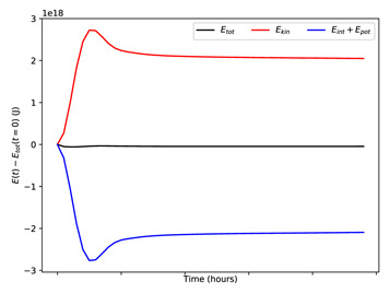
Figure 12. Total, internal plus potential, and kinetic energy in the gravity wave experiment, as a function of time, for N = 0.01 s−1 and nv = 1. Compare with Figure 6 in Tomita & Satoh (2004).
Download figure:
Standard image High-resolution image5. Comparison of THOR with Shallow and Quasi-hydrostatic Approximations
5.1. Earth-like Case with Double-gray Opacity
Here we present a dry Earth-like case to compare to the Held–Suarez test and validate the double-gray radiative transfer scheme. Input parameters are given in Table 4. We utilize optical depth profiles for the short-wave and long-wave radiation in the same style as Frierson et al. (2006) and Heng et al. (2011a), with nsw = 2, nlw = 4, τsw = 0.2, τlw,eq = 6, and τlw,pole = 1.5. In this case, the insolation, or the distribution of incident solar/stellar radiation at the top of the atmosphere, is given by

where S0 = 1367 W m−2, ϕ is the latitude, λ is the longitude, and the angle α at time t is

Here Ω = 7.292 × 10⁻⁵ is the rotation rate and norb = 1.98 × 10⁻⁷ is the orbital mean motion. This insolation pattern assumes a zero eccentricity orbit and zero obliquity but resolves the diurnal cycle. With zero eccentricity, the mean motion n is simply the angular velocity of the planet about the Sun. In a future work, we will generalize the insolation to arbitrary orbital and rotation states.
The first case is nonhydrostatic, deep (NHD) without dry convective adjustment (Figure 13). The second case is NHD with dry convective adjustment (Figure 14). Comparing the two cases, we can see that without dry convection there is clear spurious heating at ∼20°–30° latitude. With convective adjustment enabled, we produce a temperature profile much more similar to the cases in Heng et al. (2011a). As in that work, we see that the potential temperature profile, in the case without convective adjustment, is unstable near the surface at latitudes ≲50°. The convective adjustment scheme rectifies the situation and cools the near-surface region near ∼20°–30° latitude.
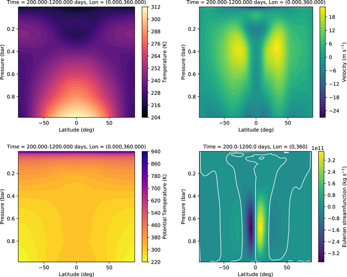
Figure 13. Zonal- and time-averaged quantities from the Earth-like, NHD simulation, without convective adjustment enabled. Top left shows the temperature, top right the zonal wind speed, bottom left the potential temperature, and bottom right the mass stream function (positive values indicate clockwise motion). The white line in the bottom right panel is the zero pass contour.
Download figure:
Standard image High-resolution image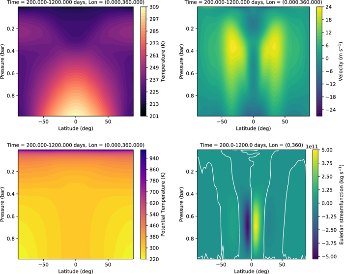
Figure 14. Zonal- and time-averaged quantities from the Earth-like, NHD simulation, with convective adjustment enabled. Top left shows the temperature, top right the zonal wind speed, bottom left the potential temperature, and bottom right the mass stream function (positive values indicate clockwise motion). The white line in the bottom right panel is the zero pass contour.
Download figure:
Standard image High-resolution imageIn both cases, we see jet streams form at ϕ ∼ 30° and P ∼ 0.4 bars (top right panels of Figures 13 and 14). There is a hint of a second, weaker stream in each hemisphere at ∼60°. The Eulerian mass stream function (bottom right panels of Figures 13 and 14) is similar in the two cases. We see strong thermally direct cells (Hadley cells) at the equator, and weaker indirect cells adjacent to these. These overturning cells are narrower in latitude than the real Hadley and Ferrel cells seen on Earth. We speculate that this may be a consequence of the lack of a hydrologic cycle in the current version of our model, as narrow Hadley cells were also observed in the dry simulations of Heng et al. (2011b), compared with, for example, Merlis & Schneider (2010).
We calculate the Eulerian mass stream function using the following relation:

where Ψ is the stream function, r0 is planet radius (at the model bottom), g is the gravity, and ![$\overline{[v]}$](https://content.cld.iop.org/journals/0067-0049/248/2/30/revision1/apjsab930eieqn123.gif) is the time and zonally averaged meridional velocity. Implicit in this definition is hydrostatic balance; in the nonhydrostatic model, this condition is not exactly satisfied. However, the simulation is at all times near enough to hydrostatic equilibrium that there is little difference between in Ψ as calculated above compared to a calculation based on Equation (4.1) of Peixóto & Oort (1984), which does not assume hydrostatic balance.
is the time and zonally averaged meridional velocity. Implicit in this definition is hydrostatic balance; in the nonhydrostatic model, this condition is not exactly satisfied. However, the simulation is at all times near enough to hydrostatic equilibrium that there is little difference between in Ψ as calculated above compared to a calculation based on Equation (4.1) of Peixóto & Oort (1984), which does not assume hydrostatic balance.
We compare the model run using the QHD and hydrostatic, shallow (HSS) approximations to the NHD case, all with convective adjustment enabled. Figure 15 shows the difference in temperature and zonal wind for the QHD and HSS simulations from the NHD case. Over most of the model domain, the differences are relatively small, on average. The largest differences occur in wind speeds in the upper atmosphere between the HSS case and NHD cases. This suggests that nonhydrostatic effects and the geometric corrections for a deep atmosphere are unimportant in this regime, at least in terms of the global average state of the atmosphere, but that the geometric corrections are more important than nonhydrostatic effects.
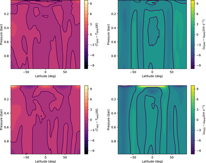
Figure 15. Residuals between the QHD or HSS and the NHD Earth-like simulations. The top panels compare the temperature (left) and zonal wind (right) for the QHD case, and the bottom panels compare the same for the HSS case. Departures from the NHD simulation are greatest at low pressures; in the lower atmosphere, the average temperatures and wind speeds are very similar.
Download figure:
Standard image High-resolution imageWe have run a single NHD case at glevel = 6, corresponding to a horizontal resolution of ∼1°. The output (not shown) is qualitatively very similar to the glevel = 5 case, though, as we discuss below, the simulation conserves mass to slightly less precision than the lower-resolution cases.
Lastly, we compare several diagnostics for the Earth-like simulations. Figure 16 shows the evolution of the global atmospheric mass, energy, and axial angular momentum. We hope to conserve the total mass; the energy and angular momentum evolve owing to input from the stellar radiation and are thus more diagnostic of convergence. The simulations at resolution ∼2° all conserve mass to a similar precision, a few parts in 1012 over 1200 days. The simulation at resolution of ∼1° does slightly worse in this respect. In all cases, the model reaches a steady state in ∼200–300 days, after which the total energy and axial angular momentum stay roughly constant.
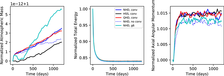
Figure 16. Evolution of the total mass, energy, and axial angular momentum in the Earth-like cases. Solid blue is the NHD case with convective adjustment, dotted blue is the NHD case without convective adjustment, red is the QHD case with convective adjustment, and black is the HSS case with convective adjustment. Cyan shows the NHD case at glevel = 6, or a horizontal resolution of ∼1°; all other cases had glevel = 5 (∼2° resolution).
Download figure:
Standard image High-resolution image5.2. HD 189733 b
Here we show a comparison of QHD and NHD simulations of the hot Jupiter HD 189733 b. The input parameters are summarized in Table 4. Simulations including the shallow approximation (HSS) are very similar to the QHD simulations; thus, we stick here to a comparison of QHD and NHD. The largest differences in flow for this planet occur between the QHD and NHD simulations, indicating that the primary source of the differences described below is the term Dvr/Dt, the Lagrangian derivative of the vertical velocity.
Figure 17 shows the zonally and temporally averaged temperature and zonal wind speed during the last 1000 days of the NHD and QHD simulations. The overall temperature structure is very similar between the two cases. The zonal wind speed plots indicate the presence of superrotation, as expected, and the overall structure is similar. However, the maximum velocities of the jets differ by ∼5%, broadly consistent with the comparison between the "Prim" and "Full" simulations of Mayne et al. (2017). While that study compared simulations using the primitive equations with the full nonhydrostatic equations, the sole difference between our simulations here is the neglect of the material derivative of the vertical velocity, Dvr/Dt, and the hyperdiffusive term,  , in the QHD case. This results in a difference of the maximum jet speed, likely because the 3D representation of waves has been modified. Though the difference is small at this resolution, it becomes more pronounced in the higher-resolution simulations, as we describe shortly.
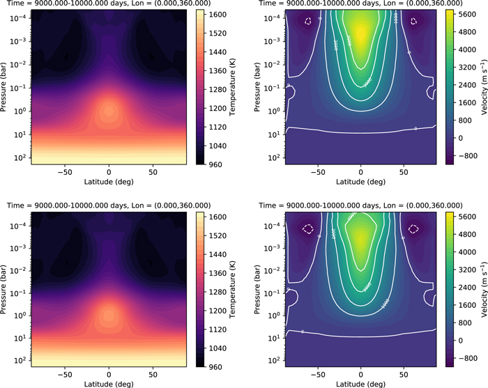
Figure 17. Zonally averaged temperature and zonal wind speed for simulations of HD 189733 b at ∼4° resolution. The top panels show the NHD case, and the bottom panels show the QHD case. All quantities are averaged over the last 1000 (Earth) days of the 10,000 day simulation.
Download figure:
Standard image High-resolution imageFigure 18 shows the zonally and temporally averaged potential temperature and Eulerian mass stream function of the NHD and QHD cases. Though the dry convection scheme is enabled in these simulations, it likely has very little effect, as everywhere the atmosphere is quite stable, as indicated by the potential temperature structure. Though this quantity is averaged over longitude, local profiles of the potential temperature at different longitudes near the equator also show stability. In the plots for the mass stream function, we see thermally indirect overturning cells at the base of the equatorial jet, as also seen in Charnay et al. (2015) and Mendonça et al. (2018a). Thermally direct cells appear adjacent to the indirect cells at higher latitudes. Overturning in the upper atmosphere is weak in comparison and indiscernible on this scale.
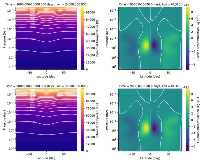
Figure 18. Zonally averaged potential temperature and stream function for simulations of HD 189733 b at ∼4° resolution. In the stream function plots, positive values indicate clockwise motion. The top panels show the NHD case, and the bottom panels show the QHD case. All quantities are averaged over the last 1000 (Earth) days of the 10,000 day simulation.
Download figure:
Standard image High-resolution imageFigure 19 shows snapshots (at 10,000 days) of the temperature and horizontal wind speeds along isobars for the NHD and QHD simulations. At 0.1 bars and above (in altitude), in the region of the superrotational jet, we see the characteristic chevron shape and eastward hot spot offset associated with hot Jupiters. The wind vectors indicate eastward motion and that the gas is pushed away from the substellar point (at 0° longitude). At 1 mbar, we see return flow on the night side at high latitudes, which results in convergence on the equator at the eastern terminator and the recognizable chevron shape. The NHD and QHD simulations show only minor differences in temperature, but the velocities are slightly higher in the NHD case. Standing Rossby waves are easily discernible at these pressure levels. At the 10 bar level, flow at the equator is retrograde, though comparatively sluggish (∼10 m s−1).
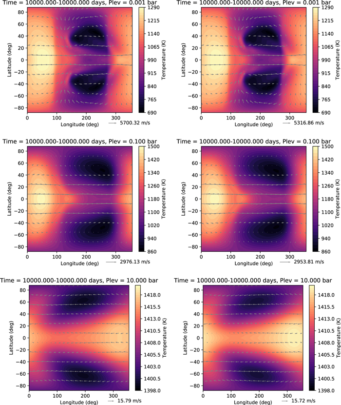
Figure 19. Snapshots at 10,000 days of the temperature (color) and horizontal winds (arrows) on isobaric surfaces for simulations of HD 189733 b at ∼4° resolution. The left panels are the NHD simulation, and the right panels are the QHD simulation. The substellar point is at 0° longitude, 0° latitude.
Download figure:
Standard image High-resolution imageFigure 20 shows the temperature and zonal wind speed, as in Figure 17, but for simulations with a resolution of ∼2°. Temperatures shows a similar pattern to the ∼4° resolution simulations, but the superrotational jet has increased in speed and has broadened in latitude, pushing the return flow toward higher latitudes. The increase in velocity is likely due to better resolution of waves that carry angular momentum toward the equator. The peak velocity of the NHD simulation is ∼20% greater than in the QHD simulation, similar to the effect seen at ∼4° resolution. The potential temperature and stream function for the  simulations are shown in Figure 21. The temperature and wind speeds along isobars are shown in Figure 22.
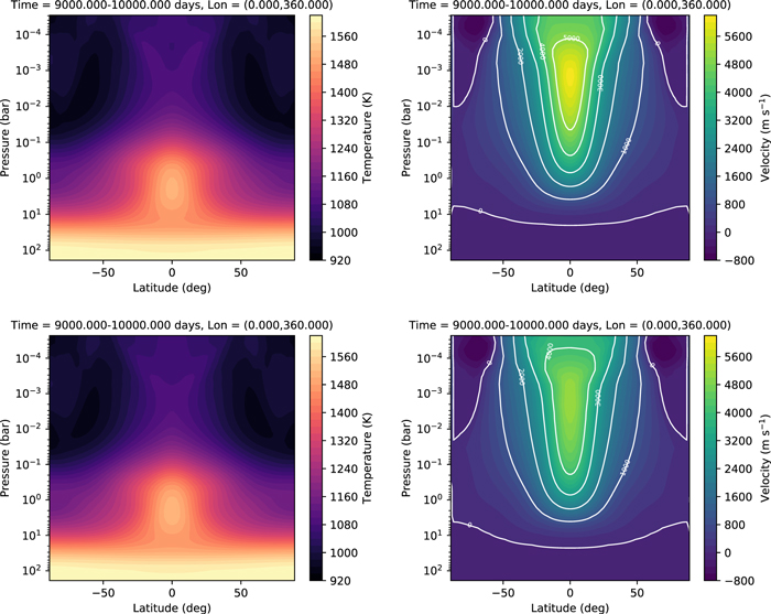
Figure 20. Zonally averaged temperature and zonal wind speed for simulations of HD 189733 b at ∼2° resolution. The top panels show the NHD case, and the bottom panels show the QHD case. All quantities are averaged over the last 1000 (Earth) days of the 10,000 day simulation.
Download figure:
Standard image High-resolution image
Figure 21. Zonally averaged potential temperature and stream function for simulations of HD 189733 b at ∼2° resolution. In the stream function plots, positive values indicate clockwise motion. The top panels show the NHD case, and the bottom panels show the QHD case. All quantities are averaged over the last 1000 (Earth) days of the 10,000 day simulation.
Download figure:
Standard image High-resolution image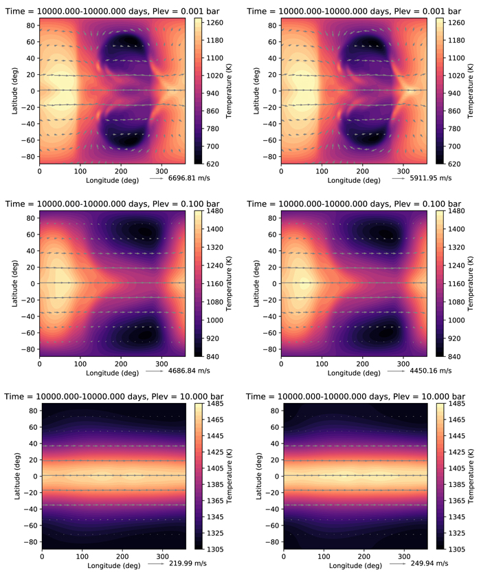
Figure 22. Snapshots at 10,000 days of the temperature (color) and horizontal winds (arrows) on isobaric surfaces for simulations of HD 189733 b at ∼2° resolution. The left panels are the NHD simulation, and the right panels are the QHD simulation. The substellar point is at 0° longitude, 0° latitude.
Download figure:
Standard image High-resolution imageFigure 23 shows the zonal and vertical velocities in a latitudinal band along the equator, averaged over the last 1000 days, for the NHD and QHD simulations at ∼4° resolution. Here we have used altitude as our vertical coordinate to avoid extrapolation at the top of the model. The values are averaged over a 20° latitudinal band weighted by  , where ϕ is the latitude. Zonal winds are highest on the night side (longitudes 90°–270°) toward the western terminator. As the flow approaches the day side, it slows because of the increase in pressure. Vertical velocities are slow everywhere in comparison to the horizontal winds, though the figures show a lot of structure. Upwelling and downwelling occur, for example, side by side along the western terminator. Upwelling dominates on the day side of the planet, with downwelling on the night side, most prominently east of the eastern terminator. Figure 24 shows equatorial temperatures in the same style, comparing the NHD and QHD cases.
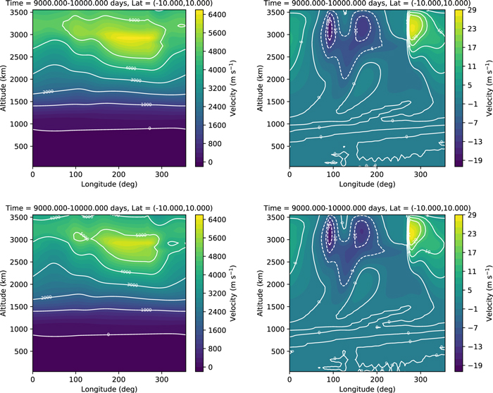
Figure 23. Zonal (left) and vertical (right) wind speeds averaged over a 20° latitude band centered about the equator for simulations of HD 189733 b at ∼4° resolution. The top panels are the NHD case, and the bottom panels are the QHD case. All quantities are averaged over the last 1000 (Earth) days of the 10,000 day simulation.
Download figure:
Standard image High-resolution image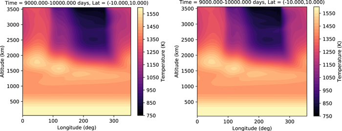
Figure 24. Temperatures averaged over a 20° latitude band centered about the equator for simulations of HD 189733 b at ∼4° resolution. The left panel is the NHD case, and the right panel is the QHD case. Temperatures are averaged over the last 1000 (Earth) days of the 10,000 day simulation.
Download figure:
Standard image High-resolution imageThe same quantities are shown for the ∼2° simulations in Figures 25 and 26. While the temperature structure is largely unchanged from the ∼4° cases, the velocities have changed more significantly. In particular, there is now a strong difference between the peak zonal winds in the NHD and QHD cases. The zonal wind speeds have increased, the vertical wind speeds have slightly decreased, and the flow now extends deeper into the atmosphere, as also seen in Figure 20.
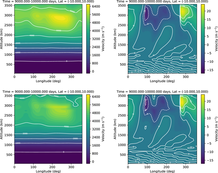
Figure 25. Zonal (left) and vertical (right) wind speeds averaged over a 20° latitude band centered about the equator for simulations of HD 189733 b at ∼2° resolution. The top panels are the NHD case, and the bottom panels are the QHD case. All quantities are averaged over the last 1000 (Earth) days of the 10,000 day simulation.
Download figure:
Standard image High-resolution image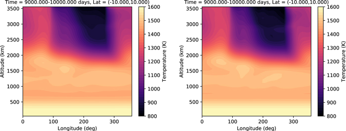
Figure 26. Temperatures averaged over a 20° latitude band centered about the equator for simulations of HD 189733 b at ∼2° resolution. The left panel is the NHD case, and the right panel is the QHD case. Temperatures are averaged over the last 1000 (Earth) days of the 10,000 day simulation.
Download figure:
Standard image High-resolution image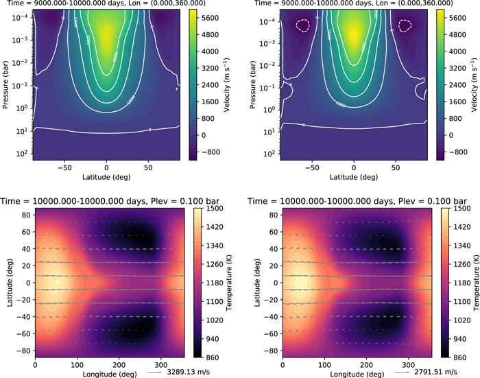
Figure 27. Zonally averaged wind speed (top) and temperature at the photosphere (bottom) for simulations of HD 189733 b using different numerical dissipation strengths. The left panels correspond to Dhyp = Ddiv = 4.99 × 10⁻³, and the right panels correspond to Dhyp = Ddiv = 1.499 × 10⁻². Compare to the NHD simulations in Figures 17 and 19.
Download figure:
Standard image High-resolution image6. Effects of Numerical Dissipation
Here we examine the effects of numerical dissipation on the simulations of HD 189733 b. We perform two additional simulations, at resolution ∼4°, with Dhyp = Ddiv = 4.99 × 10⁻³ and Dhyp = Ddiv = 1.499 × 10⁻² (or 0.5 and 1.5× the original value of 9.97 × 10⁻³). Zonal winds and temperatures at 0.1 bar are shown in Figure 27. The peak averaged zonal wind speed is similar in these cases to the simulation presented in Section 5; however, some differences are apparent. The equatorial jet appears wider and penetrates deeper into the atmosphere in the case with weaker dissipation. Calculation of the phase curve indicates that the change in diffusion produces a small shift (≈3°) in the hot spot offset. Thus, this feature appears to be largely insensitive to the numerical dissipation, as also found in Heng et al. (2011a).
We have run one final simulation to test the effect of sponge layer drag at the top boundary. In this simulation, the sponge layer was removed after 5000 days; everything is otherwise identical to the NHD case at ∼4° resolution. The purpose here is to establish whether the sponge layer can be removed once the model has spun up and flow is established or if the model simply crashes. Then, if the model remains stable, we would like to see how the flow changes in the absence of this numerical damping. In this case, the model does not crash, and the results are shown in Figure 28.
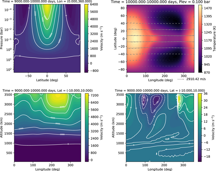
Figure 28. Zonal-mean zonal velocity (top left), temperature and horizontal winds at P = 0.1 bars (top right), zonal winds along the equator (bottom left), and vertical winds along the equator (bottom right), for HD 189733 b, when the sponge layer drag is removed after 5000 days.
Download figure:
Standard image High-resolution imageThe zonal-mean zonal wind speed in this case is increased compared to the case in Figure 23. The primary contribution occurs on the night side of the planet. Further, the wind speed increases monotonically with height, and the maximum appears right against the upper boundary. Otherwise, the basic structures of the flow remain similar to the case with the sponge layer continuously enabled. There are minor changes in the pattern of the vertical winds, because of the increased nightside zonal wind speed, though the main trends remain the same: downwelling occurs on the night side of the planet, whereas upwelling occurs on the day side and is strongest at the western terminator.
In Figure 29 we compare the evolution of global quantities for all of our simulations of HD 189733 b: the total atmospheric mass, the total energy (internal, kinetic, and potential), and the superrotation index (Read 1986). The superrotation index, a measure of the axial angular momentum in excess of the solid-body rotation, is calculated at each point in time as

where the angular momentum at the ith grid point and jth level, lij, is given in Equation (63), and the solid-body rotation angular momentum (i.e., the angular momentum at each location if the wind speed was zero) is

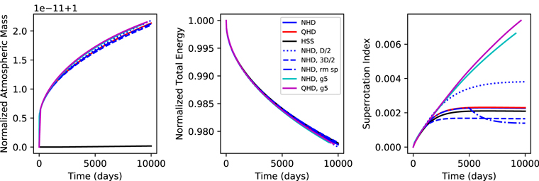
Figure 29. Evolution of the total mass, energy, and superrotation index for the HD 189733 b simulations. Solid curves correspond to simulations with Dhyp = Ddiv = 9.97 × 10⁻³. Dark-blue lines are the NHD simulations at ∼4° resolution; cyan is the NHD simulation at ∼2°; red and black are, respectively, the QHD and HSS simulations at ∼4°; and magenta is the QHD simulation at ∼2°. Three additional simulations are shown: NHD with Dhyp = Ddiv = 4.99 × 10⁻³ (dark-blue dotted), NHD with Dhyp = Ddiv = 1.499 × 10⁻² (dark-blue dashed), and NHD with Dhyp = Ddiv = 9.97 × 10⁻³ and the sponge layer removed after 5000 days (dark-blue dashed–dotted).
Download figure:
Standard image High-resolution imageIdeally, the atmospheric mass should be conserved. In practice, there is a slow drift due to numerical errors. In all of our simulations of HD 189733 b, mass is conserved to a few parts in 1011, as shown in Figure 29. This is close to machine precision for hundreds of thousands of time steps. Conservation is more than an order of magnitude better in the HSS simulation—it would seem that there is some increased numerical error associated with the curvature components of the operators. In any case, the errors are reasonably small.
The total energy is not expected to be conserved over the entire simulation, but ideally it would approach steady-state values as the simulation advances. The main reason for this is that the initial conditions are not in radiative equilibrium and it takes many thousands of days of simulation time to bring the entire atmosphere to this equilibrium. In practice, energy is also continually lost because of the numerical dissipation (see Section 4.3)—as explained earlier, we do not artificially inject dissipated energy back into heat (see, e.g., Rauscher & Menou 2012). However, this error is likely to be small compared to the radiative imbalance. We have several key developments in progress to address energy conservation in THOR. First, we are developing better initial conditions, which will start the model closer to radiative equilibrium. Second, we are exploring the use of alternate forms of the thermodynamic equation, for example, the equation for total energy. We will present these developments in a future work.
Axial angular momentum would also be conserved in an ideal simulation. As with the mass and energy, numerical dissipation and integration errors lead to a gradual drift of the total axial angular momentum. This can be seen in the superrotation index, which is a measure of the change in axial angular momentum in time. The drift in angular momentum is positive because the numerical dissipation is largest in the deep atmosphere, where the flow is retrograde (Mendonça 2019). In all our cases, the total change is less than 10%, which is acceptable in comparison with other GCMs (see, e.g., Polichtchouk et al. 2014).
The superrotation index can be interpreted as a measure of convergence (Mendonça 2019). This value plateaus (in log-space) as the model approaches steady state. In the low-resolution simulations, this is reached at ∼2500–3000 days. The superrotation index of the high-resolution simulations continues to increase, indicating that after 10,000 days these simulations are still not fully converged, consistent with the fact that the equatorial jet continues to deepen in time.
Interestingly, the NHD simulation in which the sponge layer is removed at 5000 days begins to lose angular momentum much faster than the others. It seems that allowing for greater reflection of waves of the top boundary causes an increase in the total dissipation occurring in the atmosphere. It may thus be more desirable to retain the sponge layer damping in such simulations, despite the fact that it is an additional artificial component to the model.
Figure 30 compares the maximum zonal wind speed across the suite of HD 189733 b simulations. The zonal flow develops very quickly in the upper atmosphere and changes very little after ∼2000 days in all simulations. In the ∼2° resolution (glevel = 5) simulations, the peak zonal winds are unaffected by the continued spin-up of the deep regions, indicating that flow in the upper atmosphere is converged, even though the lower atmosphere is not.
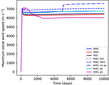
Figure 30. Maximum zonal wind speed as a function of time for the HD 189733 b simulations.
Download figure:
Standard image High-resolution image7. Summary
Here we have presented a suite of simulations using THOR. We have demonstrated how the model performs under a range of conditions. Despite the relative simplicity of the model (for a GCM), we reproduce important features of Earth's atmosphere, such as the temperature structure, zonal flow, and Hadley circulation. We have also reproduced the general features of several benchmarks for dynamical cores: a synchronously rotating Earth, a deep hot Jupiter, and wave tests previously presented in Tomita & Satoh (2004). We can also reproduce the dominant features of hot Jupiter atmospheres, such as the day/night temperature contrast and the equatorial superrotation.
The flexibility of THOR has allowed us to test the impact of commonly used approximations, like hydrostatic balance and shallow geometry, for an Earth-like case and a hot Jupiter. For the Earth-like case, the shallow approximation makes the largest difference in the results, though neither the QHD nor the HSS solution departs strongly from the full NHD simulation. While the approximations have minor consequences for the Earth-like case, we see a 15%–20% change in the peak zonal winds when the QHD approximation is made in our hot Jupiter case. Scale analysis indicates that the Dvr/Dt term (neglected in the QHD approximation) is four orders of magnitude smaller than the pressure gradient and gravitational acceleration, suggesting that the QHD approximation is valid. Comparing the Earth-like and hot Jupiter cases, Dvr/Dt ∼ 10−7 for Earth and ∼10−3 for HD 189733 b, while the dominant terms (1/ρ dP/dz and g) are ∼10 m s−2 for both planets. Thus, while the QHD approximation is good in both cases, the error is larger for the hot Jupiter. We suspect that the neglect of this term changes the behavior of waves that transport angular momentum, resulting in a difference in zonal wind speed. The vertical velocities are relatively unchanged.
We have also explored the consequences of numerical dissipation in our hot Jupiter case. Numerical dissipation makes a small difference in the overall zonal flow and the location of the peak in the thermal emission. Though the effects of modeling choices appear relatively minor, as observational data improve, it may be possible to constrain physical processes in the models, such as whether nonhydrostatic effects are significant enough to influence the bulk atmospheric circulation of hot Jupiters.
This is the first major upgrade to the open-source THOR GCM. The version consolidates physics modules that were developed in Mendonça et al. (2018a, 2018b) and makes them available to the public, along with major improvements in code design, user-friendliness, and plotting tools. The simulations presented in this work are not intended as a step forward in scientific knowledge, but as benchmarks or signposts for the THOR model. Our simulations of a dry Earth-like planet compare well with previously published works (Merlis & Schneider 2010; Heng et al. 2011a, 2011b). More realistic simulations of terrestrial planets will require a more sophisticated scheme for turbulence in the lower atmosphere (Obukhov 1971; Mellor & Yamada 1982; Galperin et al. 1988; Frierson et al. 2006), a more realistic representation of convection (Betts 1986; Betts & Miller 1986; Ding & Pierrehumbert 2016), and the effects of condensation (Frierson 2007; O'Gorman & Schneider 2008). Our hot Jupiter simulations also compare well with prior works (Showman & Guillot 2002; Cooper & Showman 2005; Rauscher & Menou 2010; Heng et al. 2011a; Mayne et al. 2017), in that we observe equatorial superrotation with wind speeds ∼5 km s−1. We have not included algorithms capable of resolving shock formation in the atmosphere or subgrid shear-driven turbulence (Goodman 2009; Li & Goodman 2010; Heng 2012; Fromang et al. 2016), clouds (Heng et al. 2012; Parmentier et al. 2013), or magnetically induced drag (Perna et al. 2010; Menou 2012; Rauscher & Menou 2012; Batygin et al. 2013) that may be important in these planets.
We acknowledge financial support from the Swiss National Science Foundation, the European Research Council (via a Consolidator Grant to K.H.; grant No. 771620), the PlanetS National Center of Competence in Research (NCCR), the Center for Space and Habitability (CSH), and the Swiss-based MERAC Foundation.
We would also like to thank Daniel Kitzmann, Yohai Kaspi, Jonathan Mitchell, Graham Lee, Mark Hammond, and Nathan Mayne for helpful discussions. Enormous thanks to the anonymous referee for the extremely constructive review. Thanks also to Brett Morris for help with and management of the Github repository.
Appendix A: Deep Hot Jupiter Temperature Profiles
The equilibrium profiles utilized in Section 4.2 and shown in Figure 6 for the deep hot Jupiter benchmark test are given by
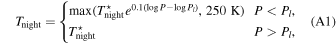
and
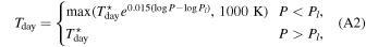
where Pl = 1 mbar. Polynomials for  and
and  in the equations above are
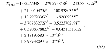
and
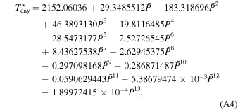
where  .
.
Appendix B: Code Improvements
We have implemented a number of coding improvements since the original release of THOR. Chief among these is the insurance of binary reproducibility, i.e., separate runs using identical initial conditions will produce identical results down to machine precision. Briefly, we describe coding procedures that ensure this property.
The primary change is the elimination of atomic addition. Atomic addition can be used in the CUDA code to ensure that parallel threads operating on the same data (and thus the same memory location) do not interfere with each other. The problem with standard addition in parallel is that reading and writing are done as separate operations, so that if multiple threads read and write to the same location, the threads may read the data at the same time (thus beginning operations with the same values) but only the last thread to write will update the sum—this is known as a "race condition." Atomic addition ensures that reading and writing are treated as a single operation; thus, threads do not interfere with each other and the computation can be done correctly.
The trouble with atomic addition is not that it is inaccurate but that there is simply no way for the machine to guarantee the order that the threads operate. Thus, because of machine round-off error, one may get a slightly different end result each time the code is run, depending on the pseudo-random order in which the threads perform the operations. Further, atomic addition can result in code slow-down as threads are forced to wait for other threads to finish their operations.
The alternative, which ensures that the summation is done correctly and that the order of operations is always the same, is "reduction addition" (see, e.g., Appendix A.1 of Sanders & Kandrot 2010). The concept is illustrated in Figure B1 (left). For an array a consisting of elements a0, a1, a2, ..., an, we first add pairs of elements (not necessarily adjacent as shown in Figure B1), resulting in an array with half the length of the original. Then, we again sum pairs of elements. The process can be repeated until the one element remains, which is the final sum of the array.
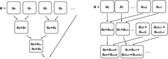
Figure B1. Concept of reduction addition used for summing over an array. Left: pairs of array elements are added iteratively, reducing the size of the array at each iteration, until one element remains (which is the total sum). Right: reduction addition on one block of the GPU adds the array elements separated by i, where i is a large power of 2, until the only total in each block remains. The totals from the blocks are then summed on the CPU to produce the total sum of the array.
Download figure:
Standard image High-resolution image
Parallelizing the process on a GPU is somewhat more complicated. First, we subdivide the array of length n into subarrays of length 2i, where i must be a power of two. The block size on the GPU is then i. The number of blocks must be long enough to cover the entire array, that is,  . For
. For  , the blocks extend past the length of the array, so the end of the array is padded with zeros. Each block will execute i threads, which each add two numbers (not adjacent pairs, in this case), aj + ai + j, where j represents the thread number. On each block, we then have an array of length i/2. We then execute i/2 threads in each block, which add the pairs of numbers
  , where a' is the new array, and repeat until only one element is left in each block, dividing the array length by two each iteration. Finally, the sum from each block is added sequentially on the CPU to produce the final summation of the array. The first two iterations of this process are illustrated in Figure 1 (right panel).
In THOR, reduction addition is used, for example, in the computation of global quantities (Section 3) and of the zonal averages used in sponge layer damping (Section 2.4). Parallel reduction is performed in  steps.
Additional code improvements include the following:
- 1.Physical processes independent of the dynamical core (fluid equations) have been modularized. Currently, the physics module consists only of gray radiative transfer, but future releases will also contain chemical tracers and boundary layer drag (in development). The purpose of the module structure is to facilitate coupling with external models or to allow the development of alternatives for the same physical processes. In the near future, this will be used to couple THOR with the radiative transfer model HELIOS (Malik et al. 2017, 2018). Each module is given its own set of configuration options and outputs and is responsible for reading and writing these. At designated points throughout the primary code of THOR, the code checks to see whether any physics modules need to be called, and the necessary values (state variables) are passed to these modules. The dynamical core then receives back a set of fluxes that are incorporated into the fluid equations. This structure allows for modules to be modified, omitted, or replaced without the need to modify the primary code of THOR.
- 2.Initial conditions are now set entirely in external configuration files. The previous version of the model required separate compilations for every change to the initial conditions, no matter how minor. Basic parameters, such as the physical characteristics of a planet or modeling choices, are set in a text file, while more involved properties, such as a nonisothermal T-P profile or a 3D wind field, can be specified by modifying binary input files using the Python code in our repository.
- 3.The Python code for plotting and regridding the icosahedral grid is now included in the repository. This code utilizes the NumPy (Oliphant 2006), SciPy (Jones et al. 2001), Matplotlib (Hunter 2007), h5py,5 PyCUDA (Klöckner et al. 2012), and PySHTools (Wieczorek & Meschede 2018) libraries. In order to produce data that plotting algorithms can utilize, it is necessary to interpolate from the icosahedral grid onto a latitude-longitude grid. This is done utilizing our own PyCUDA implementation of the Möller–Trumbore algorithm (Möller & Trumbore 1997) and properties of the icosahedral grid indexing. If desired, the vertical coordinate can be changed from altitude to pressure via interpolation, prior to the horizontal regridding, such that the horizontal interpolation is done along isobars. We often use this feature in this work.
- 4.Compilation of the model is now more flexible and user-friendly. The compiling process can now auto-detect the necessary GPU specifications and handles dependencies in a more robust fashion. The location of the HDF56 libraries, for example, can be auto-detected.
- 5.A number of debugging and performance testing tools are now built into the model and are selectable at compile time. These can be used to test for binary reproducibility or to check the magnitude of differences produced by code changes.
Footnotes
- 4
THOR is available at https://github.com/exoclime/THOR.
- 5
- 6