Quaia, the Gaia-unWISE Quasar Catalog: An All-sky Spectroscopic Quasar Sample

While performing its all-sky survey of the Milky Way, the Gaia satellite (Gaia Collaboration et al. 2016) also observed millions of extragalactic objects. These sources—both quasar and galaxy candidates—were first released in Gaia DR3 (Gaia Collaboration et al. 2023a, 2023b). Gaia obtained BP/RP spectra of the sources, which are low-resolution spectra with relatively narrow wavelength ranges; the BP covers 330–680 nm and has 30 ≤ R ≤ 100 and the RP covers 640–1050 nm (Carrasco et al. 2021) with 70 ≤ R ≤ 100. The raw spectra are not released by Gaia (besides a small subsample—the rest will be released in Gaia DR4), but redshift estimates and other derived information are contained in the catalogs.

The quasar candidates were selected based on multiple classifiers and criteria, described in detail in Gaia Collaboration et al. (2023a). The majority (5.5 million) of the quasar candidates were identified with the Discrete Source Classifier (DSC) module (detailed in Delchambre et al. 2023, a machine-learning model that takes as input the source's BP/RP spectrum, G-band magnitude, G-band variability, parallax, and proper motion, and outputs a class label trained on SDSS spectroscopic classifications. Given these SDSS labels, the results of this module will inherit many of the same selection effects as SDSS. DSC is estimated to have a completeness of over 90% and a purity of around 24% for quasars. Another machine learning model selected over 1 million sources based on their variability, as active nuclei have time-variable accretion; the model inputs were statistics of time series data in all Gaia bands as well as photometric and astrometric quantities, as detailed in Rimoldini et al. (2023). Additionally, a set of nearly 1 million sources was selected based on their surface brightness profile; this selection used existing major quasar catalogs to compile an initial list of sources, which were then processed by the Gaia surface brightness profile module (Ducourant et al. 2023). This module included quasars in the candidates catalog which passed certain criteria, including having Gaia observations covering >86% of the source's surface area and a confident assessment (positive or negative) of host galaxy presence. Finally, the 1.6 million sources used to define the Gaia-CRF3 celestial reference frame were contributed, which are based on crossmatches of Gaia to external quasar catalogs. A large fraction of sources are identified as quasars by multiple of these methods; the overlapping contributions are shown in Figure 3 of Gaia Collaboration et al. (2023a). The full quasar candidate sample contains 6,649,162 sources, ⁷ selected for high completeness, but with a low purity estimated to be around 52% (Gaia Collaboration et al. 2023a). We show the overlaps between this Gaia quasar candidate sample and other samples and subsamples used and constructed in this work in Figure 1.

Zoom In Zoom Out Reset image size

Most of the quasar candidates (6,375,063) are assigned redshifts using the Quasar Classifier (QSOC) module, which uses a chi-squared approach on the quasars' BP/RP spectra compared to composite spectra from SDSS DR12Q (Delchambre et al. 2023). We refer to these Gaia redshift estimates as z_Gaia. Many of these redshifts are determined by a single line due to the narrow spectral range, resulting in aliasing issues when lines are misidentified (see Figure 15 in Delchambre et al. 2023). An estimated 63.7% of the redshifts have ∣Δz∣ < 0.1, increasing to 97.6% for quasar candidates with no redshift warning flags (this is the case for nearly 80% of quasars with G < 18.5, but decreases to less than 20% for G > 19.5).

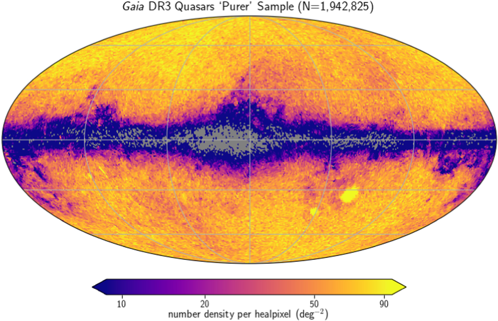
Gaia Collaboration et al. (2023a) provide a query to select a purer subsample of the quasar candidates. It requires higher quasar probability thresholds from the various classifiers and excludes surface-brightness-selected galaxies that have close neighbors. This results in 1,942,825 sources with an estimated purity of 95%; 1.7 million of these have Gaia redshifts. The sky distribution of this sample, which we call the Gaia DR3 purer sample, is shown in Figure 2. The Gaia DR3 purer sample has a low density in the Galactic plane; we speculate that this is largely due to dust extinction making sources too faint to observe at low Galactic latitudes. Gaia DR3 purer also has significant overdensities around the LMC and SMC, as the sample still contains stellar contaminants.

Zoom In Zoom Out Reset image size

For our analysis, we start with the full quasar candidate sample, rather than the Gaia DR3 purer sample or cutting on other Gaia pipeline flags, to allow greater completeness and minimize reproducing biases; we compare our catalog with the Gaia Collaboration et al. (2023a) Gaia DR3 purer subsample in Section 4.3. We construct a superset of our catalog (which is a subset of the Gaia quasar candidates sample) that contains all the information needed for catalog construction: we require that sources are in the Gaia quasar candidates table, have Gaia G, BP, and RP measurements, unWISE W1 and W2 observations (described in Section 2.2), Gaia-estimated QSOC redshifts, and a maximum G magnitude of G < 20.6. This magnitude cut was chosen to be slightly deeper than our desired catalog magnitude limit of G < 20.5, in order to provide a buffer for redshift estimation. This results in a superset with 1,518,782 sources. We call our final catalog Quaia, so we refer to this as the Quaia superset.

We use the unWISE reprocessing (Lang 2014; Meisner et al. 2019) of WISE (Wright et al. 2010) to contribute IR photometry to Gaia sources. The unWISE coadds combine data from NEOWISE (Mainzer et al. 2011) with the original WISE survey, providing a time baseline 15 times longer. Compared to the original AllWISE catalog, unWISE has deeper imaging and improved modeling of crowded fields. The unWISE catalog (Schlafly et al. 2019) contains measurements in the W1 (3.4 μm) and W2 (4.6 μm) bands for over 2 billion sources. We do not use the W3 and W4 bands as these do not go as deep as we need. We perform a crossmatch of the Gaia quasar candidate sample to unWISE sources within 1''. ⁸ We also crossmatch the SDSS training and validation samples (Sections 2.3, 2.4) to unWISE.

When combined with optical photometry, unWISE IR color information is very useful to identify quasars and distinguish them from contaminants. This photometry also contains useful redshift information; recent approaches to estimate redshifts from photometry with neural networks achieve a mean ∣Δz∣ ∼ 0.22 (Yang et al. 2017; Jin et al. 2019; Kunsági-Máté et al. 2022). In our case of redshift estimates from narrow-range BP/RP spectra, we expect IR photometry to add information that can break line identification degeneracies in order to improve estimates. We incorporate the W1 and W2 bands into both our quasar selection (Section 3.1) and redshift estimation (Section 3.2) procedures.

The SDSS released the largest spectroscopic quasar catalog in DR16 ⁹ (Lyke et al. 2020). It combines new sources from the extended Baryon Oscillation Spectroscopic Survey (eBOSS), part of SDSS-IV, with previously observed sources from earlier SDSS campaigns. The catalog contains 750,414 quasars, with an estimated 99.8% completeness (compared to the SDSS-III/SEQUELS sample of Myers et al. 2015, which has higher signal-to-noise spectra) and 98.7%–99.7% purity. We remove sources with redshift warnings, ZWARNING! = 0, as well as a handful of sources with unreasonably low or negative redshift estimates (z < 0.01). This results in 638,083 sources, which is the sample shown in Figure 1. We crossmatch these with the Gaia catalog, as well as unWISE (Section 2.2), using a maximum separation of 1'' on the sky. We remove sources with fewer than five observations in BP (phot_bp_n_obs) or RP (phot_rp_n_obs), following Bailer-Jones (2021), as well as sources that are duplicated in the SDSS star or galaxy samples (Section 2.4). This results in 343,074 sources with both Gaia and unWISE observations that pass these criteria.

We use these to calibrate the cuts to decontaminate our sample (Section 3.1); for this purpose, we only keep sources that are also in the Quaia superset (sources that are in the Gaia quasar candidates table, have all necessary Gaia and unWISE photometry, Gaia-estimated QSOC redshifts, and G < 20.6). This sample contains 246,122 quasars. We also use this sample (after applying the cuts described in Section 3.1) to train our redshift estimation model (Section 3.2). While this spectroscopic sample has quite high completeness and accurate redshift information, we note that it is still imperfect, contains selection effects, and represents only a particular definition of a quasar; these issues will propagate to our catalog.

To guide the decontamination of our catalog (Section 3.1), we compile known contaminant samples, namely galaxies and stars. For the galaxy sample, we use SDSS spectroscopic galaxies from DR18. ¹⁰ Following Bailer-Jones (2021), we include all galaxies with class label GALAXY in the SpecObj table, exclude galaxies with subclass labels AGN or AGN BROADLINE, and exclude sources with redshift warnings, zWarning=0. We crossmatch these with Gaia DR3 and unWISE with a 1'' radius, and remove sources with fewer than five observations in BP or RP, as for the SDSS quasars. We also remove apparent stellar contaminants from the galaxies sample with the cut in G − RP and BP − G from Equation (1) of Bailer-Jones et al. (2019), and additionally remove sources duplicated in the SDSS quasar or star samples. This leaves 600,897 crossmatched SDSS galaxies in our sample; 1316 of these are in the Quaia superset.

For the star sample, we also use SDSS DR18 sources, selecting objects with the class label STAR in the SpecObj table. As for the quasars and galaxies, we crossmatch these with Gaia DR3 with a 1'' radius and remove sources with fewer than five observations in BP or RP, and remove sources duplicated in the other samples. This results in a stellar sample with 482,080 crossmatched SDSS-Gaia stars, with 2276 of these in the superset.

For the decontamination procedure, we also compile a sample of sources in or near the LMC or SMC, as most of these will be stellar contaminants but have different properties than the SDSS star sample. To do this, we select all sources in the Gaia quasar candidates table that are within 3° of the center of the LMC or 1.5° from the center of the SMC. While this may include stars not actually in the LMC or SMC, we have chosen these fairly narrow radii in order to capture mostly LMC and SMC stars and a few potential quasars. Additionally requiring that these have unWISE photometry, this gives 11,770 LMC- and SMC-adjacent stars; 9927 are in the superset.

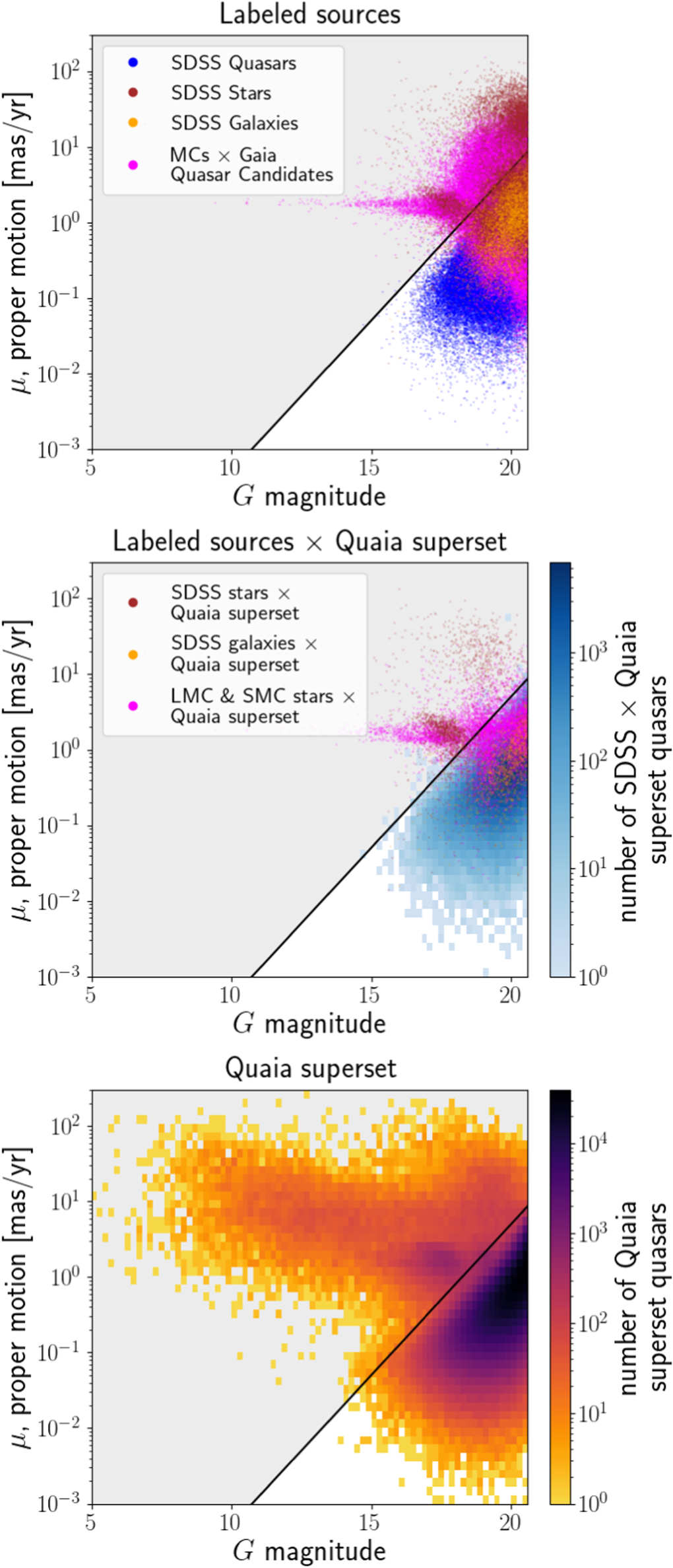
The full Gaia quasar candidate sample is known to contain a significant fraction of contaminants (stars and other non-quasars, such as galaxies). The stellar contaminants might include sources such as brown dwarfs, which have similar colors as high-redshift quasars, and potentially blue horizontal branch stars, blue stragglers, and white dwarfs, which are UV bright like lower-redshift quasars. To remove stellar contaminants, we make an initial cut on proper motion μ, as quasars should have negligible proper motions due to their large distances. The value of μ has a dependence on G, so we make a cut in this space. To guide this cut, we use labeled sources: SDSS quasars, SDSS galaxies, SDSS stars, and Gaia LMC- and SMC-adjacent stars, as described in Sections 2.3 and 2.4. The G–μ distributions of these sources are shown in the top panel of Figure 3. In the middle panel, we show the intersection of these labeled sources with our Quaia superset, which consists of sources in the Gaia quasar candidates table that have Gaia redshift estimates, complete Gaia, and unWISE photometry, and are below G < 20.6. We see that the SDSS quasars tend to have much smaller proper motions than the other types of sources, with a very linear edge to the G dependence at the high proper motion side of the distribution. Based on this, we choose the cut

$$\begin{eqnarray}&&\mu \lt {10}^{0.4(G-18.25)}\ \mathrm{mas}\,{\mathrm{yr}}^{-1}.\end{eqnarray} \tag{ 1 }$$

At G = 18.25, this corresponds to μ ≲ 2.5 mas yr⁻¹, and allows for less severe cuts at deeper magnitudes given the typically less precise astrometry. This is related to the proper motion uncertainty as a function of G, which has been quantified by Gaia (Gaia Collaboration et al. 2021). We show this cut overlaid on the Quaia superset in the lower panel of Figure 3; based on the labeled data, we can clearly pick out the populations. The proper motion cut excludes 39,470 sources, 2.6% of the superset.

Zoom In Zoom Out Reset image size

Next, we determine the color cuts based on Gaia and unWISE photometry. Generally, stars and galaxies are dim in redder, IR wavelengths compared to AGN. For instance, the eBOSS quasar target selection (Myers et al. 2015) involved linear cuts in the optical-IR, involving the SDSS g, r, and i bands and the WISE W1 and W2 bands.

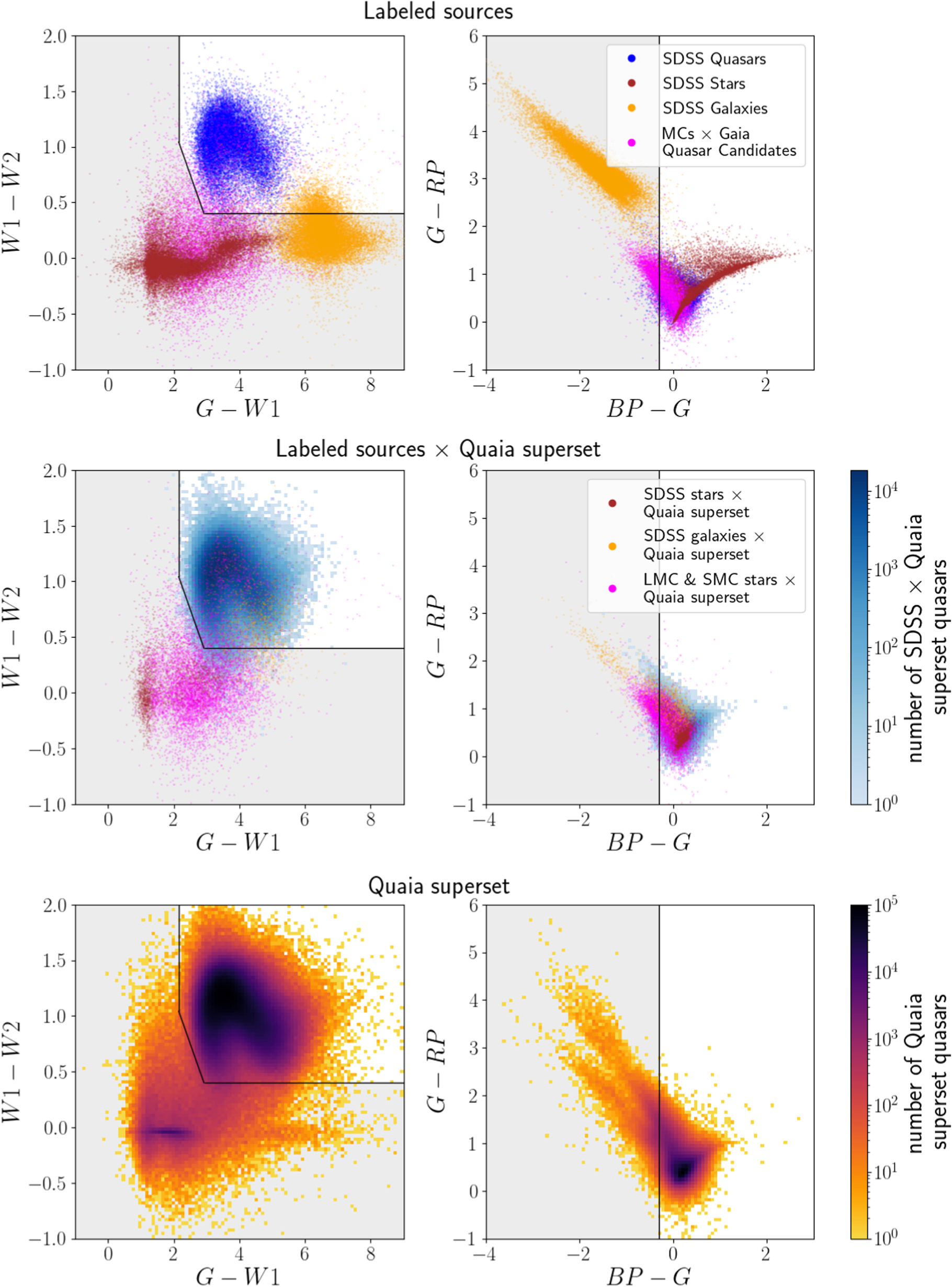
In Figure 4, we show color–color distributions for the same samples as in Figure 3. The left panel shows W1 − W2 versus G − W1 color, and the right column shows G − RP versus BP − G color. The top row, with the full labeled samples, shows that different types of sources tend to be localized to different areas of this parameter space (we show only a subset of each type for clarity). In particular, the colors involving unWISE (left panel) separate out the source types relatively clearly, demonstrating the importance of the unWISE crossmatch: SDSS quasars have very red W1 − W2, and intermediate G − W1 color, while galaxies have bluer W1 − W2 and redder G − W1 compared to quasars, and stars (both SDSS stars and stars near the LMC and SMC) are bluer in both colors. In Gaia color–color space, galaxies tend to have bluer BP − G and redder G − RP colors than the other types of sources. In the middle row of Figure 4, showing the intersection of the labeled sources with the Quaia superset, we see that the superset restrictions have eliminated many of the sources, especially SDSS galaxies and stars, though a significant number remain. (We note that it is possible that some of these SDSS galaxies do host AGN though they were not classified as such by SDSS.) The Quaia superset is shown in the bottom panel; we can see clear populations of quasars, stars, and galaxies lining up with the labeled sources. Importantly, we can see the effect of the stricter SDSS color selection in the red (high G − W1) region of parameter space into which the Gaia quasar candidates extend, but are not represented in the SDSS sample in the above panels.

Zoom In Zoom Out Reset image size

We choose to apply linear cuts in these colors to decontaminate the sample. While other works (e.g., Hughes et al. 2022) train classifiers to determine which objects are true quasars using SDSS-classified quasars as labels, we opt for simpler cuts for ease of reproducibility and to mitigate the propagation of SDSS selection effects, which may include color- and magnitude-dependent effects. We choose four cuts based on the distribution of sources in color–color space. The first is in W1 − W2, which has been shown to be useful for distinguishing quasars; for instance, Nikutta et al. (2014) demonstrated that a small crossmatched SDSS quasar sample has very red W1 − W2 = 1.2 ± 0.16, while other types of objects—namely star-forming and AGN galaxies, luminous red galaxies and stars—have bluer W1 − W2. Stars tend to have the bluest W1 − W2, with a mean of W1 − W2 = − 0.04 ± 0.03, so a cut in W1 − W2 is a reliable way to filter out stellar contaminants. We add a cut in G − W1 to filter out the bulk of the stars (including the LMC and SMC), and another in BP − G to cut out the galaxy contaminants. Finally, we find that these single color cuts were not sufficient to remove all of the LMC and SMC, so we add an additional diagonal cut in W1 − W2 and G − W1, choosing a reasonable slope.

We optimize the values (intercepts) of these four cuts with a grid search, trying values spaced out by 0.1 mag. We note that while we show the full samples in Figure 4, in practice we make the proper motion cut before optimizing the color cuts. We choose the color cuts that maximize our objective function ${ \mathcal L }$,

$$\begin{eqnarray}&&{ \mathcal L }={N}_{{\rm{q}}}-{\lambda }_{{\rm{s}}}\,{N}_{{\rm{s}}}-{\lambda }_{{\rm{g}}}\,{N}_{{\rm{g}}}-{\lambda }_{{\rm{m}}}\,{N}_{{\rm{m}}},\end{eqnarray} \tag{ 2 }$$

where N_q is the number of true quasars that make it into the catalog, N_s SDSS stars, N_g SDSS galaxies, and N_m LMC and SMC stars, and the λ parameters balance the relative ratios of each. We choose λ_s = 3, λ_m = 5, and λ_g = 1.

The optimal cuts for the objects to keep in the catalog are

$$\begin{eqnarray}&&\begin{array}{l}(G-{\rm{W}}1)\gt 2.15\\ ({\rm{W}}1-{\rm{W}}2)\gt 0.4\\ ({BP}-G)\gt -0.3\\ (G-{\rm{W}}1)+1.2({\rm{W}}1-{\rm{W}}2)\gt 3.4.\end{array}\end{eqnarray} \tag{ 3 }$$

These are shown as the black lines in all panels of Figure 4, with the gray shading indicating exclusion regions. These cuts, as well as the proper motion cuts described above, exclude ∼7% of the superset, resulting in 1,414,385 quasars in our decontaminated sample. We apply an additional magnitude cut of G < 20.5 to reduce edge effects in our redshift estimation; this constitutes our deep sample, with 1,295,502 sources. We refer to this as Quaia in the rest of this work. However, the catalog becomes less clean and reliable as we push to deeper magnitudes—due to less precise measurements and stronger systematics, notably the Gaia scanning pattern—so we produce a version of the catalog with G < 20.0 to ensure a cleaner sample. This brighter catalog has 755,850 sources, and we report most of our results on this sample throughout the rest of this work.

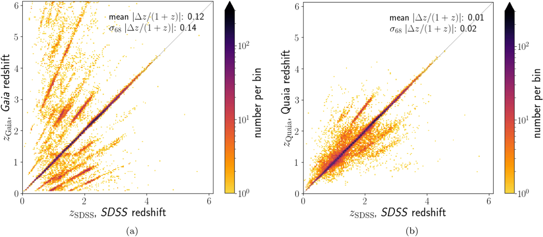
We use unWISE and SDSS data to improve the redshift estimation of the sources. Figure 5(a) shows the redshifts estimated by the Gaia QSOC pipeline z_Gaia compared to the SDSS redshifts z_SDSS for a test sample of sources from Quaia with G < 20.5; note that the 2D histogram is plotted in log-space to show the outliers more clearly. We find that of the Gaia redshifts z_Gaia, 82% (81%) agree to ∣Δz/(1 + z)∣ < 0.2 (0.1). A significant fraction of z_Gaia are highly precise: 75% agree with SDSS to ∣Δz/(1 + z)∣ < 0.01. We also clearly see bands of incorrect estimation due to line aliasing issues. Additionally, in the crossmatched sample, nearly all of the very high z_Gaia estimates (z > 4.5) are shown to be incorrect in comparison to SDSS. We note that the redshift estimation is much more accurate for sources that have no redshift warning flags set (flags_qsoc=0), as discussed in Section 2.1, but this is only true for 21% of the sources in Quaia (G < 20.5), and even including sources with flags_qsoc = 16 this leaves only 39% of sources.

Zoom In Zoom Out Reset image size

We train a kNN model on Quaia sources to estimate improved redshifts. (We also tested other models including XGBoost and a multilayer perceptron, and found that the kNN outperformed both by a small margin.) We include all sources in our decontaminated catalog (Section 3.1), which goes out to G < 20.6, in order to have a buffer beyond our desired G < 20.5 sample to reduce edge effects from the training set. The features that we train on are the Gaia redshift z_Gaia, colors constructed using Gaia and WISE photometry (G − RP, BP − G, BP − RP, G − W1, W1 − W2), the Gaia G-band magnitude, and the dust reddening E(B − V) at the location of the source. (We find that including the rest of the photometry does not make a difference in the results.) The reddening is determined with the Corrected Schlegel, Finkbeiner, & Davis dust map introduced by Chiang (2023), which corrects the standard Schlegel et al. (1998) dust map by subtracting off the contribution from the cosmic infrared background (CIB). (We also include the appropriate correction factor given by Schlafly & Finkbeiner (2011).) ¹¹ The labels are the SDSS redshifts, z_SDSS.

We use as our labeled data sources from the crossmatched SDSS DR16Q sample (Section 2.3) that are also in our decontaminated catalog Quaia, so that we train on sources drawn from the same distribution to which we will apply the model; this is 243,206 sources. We apply a 70%/15%/15% train/validation/test split. We build a k-d tree on the training set features using the KDTree implementation of sklearn. At the prediction stage, we access the K nearest neighbors of each input feature vector, first excluding neighbors with zero distance in feature space (i.e., neighbors that are in the training set). We assign the predicted label to be the median z_SDSS of the K nearest neighbors and the uncertainty to be the symmetrized inner 68% error of those neighbors. We use the validation set to tune K, and choose the value that maximizes the fraction of predicted redshifts with ∣Δz/(1 + z)∣ < 0.1, which is K = 27; we note that this value only varies at the ∼1% level for values 15 < K < 50, and is similar for other choices of ∣Δz/(1 + z)∣. Finally, we apply the model to the full Quaia and output kNN redshift estimates, z_kNN, for each source.

The results are shown in Figure 6, which shows the cumulative distribution of errors ∣Δz/(1 + z)∣ for z_{k NN} compared to that of z_Gaia (with z_SDSS as the truth) for the test set with G < 20.0. (The shapes are similar for G < 20.5, just shifted to somewhat lower accuracy.) We find that the z_kNN estimates have far fewer outliers than z_Gaia. However, the z_Gaia estimates tend to be more precise, as they use the full spectral information, while the kNN is essentially smoothing over the likeliest neighboring sources in feature space. We thus choose to combine the properties of both of these redshift estimates to obtain our final spectrophotometric (SPZ) redshifts z_Quaia in the following way. For sources for which z_Quaia and z_Gaia agree to ∣Δz/(1 + z)∣ < 0.05, we assign z_Quaia = z_Gaia to preserve the precision of the Gaia estimate. For sources for which z_Quaia and z_Gaia differ by ∣Δz/(1 + z)∣ > 0.1, we assign z_Quaia = z_kNN to preserve accuracy. In between these thresholds, we apply a smooth, linear transition to avoid hard features in our estimates. These z_Quaia estimates are also shown in Figure 6 compared to the true (spectroscopic, taken as truth for our purposes) SDSS redshifts, and we can see that these achieve nearly as high precision as z_Gaia while maintaining the high accuracy of z_kNN.

Zoom In Zoom Out Reset image size

Our z_Quaia results for the test set are shown in Figure 5(b) compared to z_SDSS, shown here for the full catalog depth G < 20.5. We find that 91% (84%) of our SPZ redshifts agree to ∣Δz/(1 + z)∣ < 0.2 (0.1), and 62% highly agree to ∣Δz/(1 + z)∣ < 0.01. We also give the bias (mean redshift error) and scatter (σ₆₈, the symmetrized inner 68% region of the redshift errors) of ∣Δz/(1 + z)∣ in the figure; our SPZ redshifts significantly decrease the bias and scatter. The SPZ estimation corrected all of the very high-z Gaia estimates, and some of the intermediate-outlying aliasing effects. We still have some catastrophic outliers due to line aliasing, but with our SPZ redshifts, we find a reduction in the number of ∣Δz/(1 + z)∣ > 0.2 (0.1) outliers by approximately three times (approximately two times) compared to the Gaia redshift estimates.

We investigate the dependence of the redshift error on the G-band magnitude in Figure 7. The fraction of redshifts with an error above various thresholds is shown as a function of samples with the given cut on G. The errors are lowest at a bright magnitude cut of G < ∼ 19.0; in this sample, sources with SPZ redshift estimates inaccurate to ∣Δz/(1 + z)∣ > 0.2 (0.1) comprise only 3% (4%) of the sample, and to the more stringent requirement of ∣Δz/(1 + z)∣ > 0.01, 12%. This outlier fraction increases steadily as fainter sources are included. For G < 20.0, 6% (10%) are inaccurate to ∣Δz/(1 + z)∣ > 0.2 (0.1), and 25% for ∣Δz/(1 + z)∣ > 0.01. Compared to the Gaia redshift estimates, the SPZ estimates z_Quaia reduce the number of ∣Δz/(1 + z)∣ > 0.2 (0.1) outliers by approximately three times (approximately two times). The choice of G cut to use in a given analysis will depend on the nature of the analysis and its sensitivity to outliers.

Zoom In Zoom Out Reset image size

We note that our finding that the unWISE IR information significantly improves redshift estimates, compared to only the optical information used in the Gaia QSOC estimates, is consistent with other photometric redshift work. For instance, DiPompeo et al. (2015) showed that including WISE mid-IR photometry in the redshift estimation of SDSS-imaged quasars results in a significant improvement in the estimates, even more so than including both GALEX near- and far-UV data and UKIDSS near-IR data. More recently, Yang & Shen (2023) compiled a photometric quasar catalog from the Dark Energy Survey (DES) DR2, combining DES optical photometry with near-IR photometry as well as unWISE mid-IR photometry; they obtained photo-zs with 92% having ∣Δz/(1 + z)∣ < 0.1 when all IR bands are used compared to 72% with only optical data. Additional photometric information at other wavelengths could further improve our estimates (as well as catalog decontamination), but is not currently available for enough sources in our Quaia catalog to be worthwhile. For instance, for the UV all-sky survey GALEX (Martin et al. 2005), crossmatches to Quaia sources are only available for 32% of the Quaia objects for near-UV observations, and when including far-UV only 16%; this significant discrepancy is largely due to the faint end of Quaia, where GALEX observations do not reach deep enough. The Pan-STARRS1 survey (Chambers et al. 2016) covers only three-quarters of the sky, with crossmatches to 75% of Quaia sources. We tested adding Pan-STARRS1 data to the redshift estimation feature set and found only a small improvement, and thus chose to prioritize keeping the full sky span of Quaia, though we make note that incorporating Pan-STARRS1 may be useful for certain applications.

Observational and astrophysical effects impact which sources we observe and their properties; this is known as the selection function. As Gaia is a space-based mission, it avoids many of the observational issues of ground-based surveys, such as seeing and airmass. However, there are still significant selection effects: for our model, we consider dust, the source density of the parent surveys, and the scan patterns of the parent surveys.

We fit a selection function model to a particular version of the catalog, namely, a particular maximum G. For the fiducial selection function we work only in terms of sky position. We make a healpix map of the catalog with NSIDE = 64 and count the number of observed catalog sources in each healpix pixel. We choose this NSIDE, which results in 49,152 pixels each with an area of ∼0.84 deg², to balance constructing a map with reasonably high resolution with ensuring a sufficient number of sources in the pixels for stable fits, as well as fitting within memory limitations for the Gaussian process fit. In the case of no selection effects (and under the assumption of isotropy), we would expect each pixel to contain roughly the same number of sources. Our goal is to model the dependence between the number of sources per pixel and the various systematics.

The systematics maps (templates) we use are shown in Figure 8. We use the dust map of Chiang (2023), and convert it to a healpix map of NSIDE = 64. To do this, we evaluate the reddening E(B − V) at the centers of pixels of a high-resolution NSIDE = 2048 healpixelization of the sphere, and apply the 0.86 correction factor proposed by Schlafly & Finkbeiner (2011). We convert these to extinction values by multiplying by R_V = 3.1, and then take the mean of all of these values within each healpixel target NSIDE = 64 map. This produces a smoothed dust extinction map on the desired scale. The result is shown in Figure 8(a); the extinction is highest around the Galactic plane, with structure extending outward.

Zoom In Zoom Out Reset image size

For the stellar distribution, we randomly select ∼10.6 million Gaia sources with 18.5 < G < 20, the magnitude range of most of our quasar sample. The vast majority of these will be true stars. (While this sample will contain some other types of objects, including possibly some quasars and other extragalactic sources, these will be orders of magnitude less numerous than stars.) We count the number of stars per NSIDE = 64 healpixel; this is shown in Figure 8(b). We also include a template of the unWISE source distribution, for which we randomly selected ∼10.6 million unWISE sources (1% of the catalog) that have flux in both W1 and W2, and have primary status (Prim = 1). We count the number of these sources per NSIDE = 64 healpixel, as shown in Figure 8(c).

In initial fits we found that the regions of the LMC and SMC are particularly poorly modeled, and that the fit is improved by including separate templates of just the LMC and SMC source density for both the Gaia and unWISE sources; this gives the model the freedom to assign different coefficients to these regions than to the overall survey source density. (The need for different coefficients could be for a number of reasons, such as a difference in stellar density, contamination, or magnitude distribution; we leave a deeper investigation of this to future work and just use this empirical finding to improve our model.) For the LMC/SMC templates, we cut out a wide region around the LMC and SMC (9° in radius around the LMC and 5° around the SMC), and subtract the background, which we approximate using the region at the same latitude but opposite longitude (mirrored across the l = 0° line) of the given source distribution map. We do not show these maps here as they are visually similar to the stellar and unWISE source density maps in the LMC and SMC regions (though with the background subtracted).

For the Gaia completeness, we use the quantity M₁₀ introduced by Cantat-Gaudin et al. (2023). ¹² M₁₀ is the median magnitude in a given sky patch of the Gaia sources with ≤10 transits across the Gaia field of view; it incorporates the effects of both the scanning law and source crowding. The actual completeness map derived by Cantat-Gaudin et al. (2023) depends on both M₁₀ and G-band magnitude; this completeness is very close to 1 for nearly all of the sky for G = 20.0, with some non-negligible incompleteness for G = 20.5. However, this completeness model is based on the full Gaia source catalog, while we expect the selection function of our quasar sample to be different. We thus use the M₁₀ map directly in our fit to capture the effects of the Gaia scanning law and source crowding specific to Quaia. We downsample the map to NSIDE = 64; this is shown in Figure 8(c).

For the unWISE scanning law, using the ∼10.6 million unWISE sources described above, we take the mean number of single-exposure images in the coadd in W1 for the sources in each NSIDE = 64 healpixel. This is shown in Figure 8(e); we can see that the scan is in strips of constant ecliptic latitude, and that there is a significant increase in observations at the ecliptic poles.

To model the selection function we use a Gaussian process, a flexible machine-learning method for regression; for a detailed treatment, see Rasmussen & Williams (2005). (We first tried a linear model and found that it gave a very poor fit, because there are significant nonlinearities between the systematics and the catalog number density.) We first scale the data: for the labels (number of Quaia sources per pixel) we work in their logarithm, and only fit for the pixels with a nonzero number of sources. For the Gaia stellar distribution, the unWISE source distribution, the unWISE scan pattern, and LMC/SMC map templates, we also take the log of the number of quasars per pixel; for the LMC/SMC map, we first replace zeros with a very small value. For all of the input feature maps, we take the mean-subtracted systematics values. We assume a Poisson error on the labels (and apply the appropriate log transformation). For the Gaussian process, we use the george software package (Ambikasaran et al. 2016). We use an exponential squared kernel k of the form

$$\begin{eqnarray}&&k({r}^{2})=\exp \left(\displaystyle \frac{-{r}^{2}}{2}\right),\end{eqnarray} \tag{ 4 }$$

where r is the distance between points in feature space. We train the Gaussian process on all of the data, optimizing the parameter vector using the BFGS solver (Fletcher 1987); this includes fitting for the mean of the labels. We finally evaluate the predicted number of sources in each pixel. Where there were no Quaia sources in the label map, we fix the prediction to zero.

To convert this to a selection function in terms of the relative completeness, we first identify clean pixels in the map having low dust extinction (A_V < 0.03 mag), low star counts (N_stars < 15), low unWISE source counts (<150), no stars or unWISE sources in the LMC or SMC, and high M₁₀ (M₁₀ >21 mag) and unWISE coadds (>150); this results in 479 pixels. We take the mean predicted number of quasars in these clean pixels, and add two times the standard deviation in these pixels to encompass the scatter. We then normalize the predicted source numbers by this value, which ensures that all final values end up being less than 1 for clarity. The result is a selection function map in terms of the relative probability of a source at a given location being included in the catalog. We emphasize that this is relative; we have not normalized it to an absolute probability so as not to make the selection function map extremely sensitive to the maximum value. We also note that this fit must be redone for each version of the catalog because it depends on the particular number density and distribution of sources.

There will be a dependence of the selection function on the G-band magnitude, as well as other quantities such as redshift. While we do not include these in our modeling or fiducial selection function map, we do release selection functions for a redshift split version of the catalog, using two redshift bins, which is important for certain cosmological analyses. The code to generate the selection function for any input catalog is also provided so that users can construct maps that meet their needs.

Quaia, the Gaia-unWISE Quasar Catalog, consists of 755,850 (1,295,502) quasar candidates with G < 20.0 (20.5). The sky distribution of Quaia for each of these magnitude limits is shown in Figure 9. The catalog covers the full sky, besides the Galactic plane, including the southern sky—most of which is not well covered by other surveys (discussed further in Section 4.3). The sky distribution is remarkably uniform, and the nonuniform imprints visually follow the selection effects that we incorporated into our selection function map, most notably the dust distribution (Figure 8(a)). Quaia also does not show an obvious overdensity around the LMC and SMC (as the Gaia DR3 purer sample does) because we have removed these with our decontamination procedure. In fact, there is now a slight underdensity of sources near the LMC; this makes sense because some quasars in that sky region are obscured by dust and confusion in the LMC, though it is possible we have also somewhat overcorrected for this and removed some true quasars.

Zoom In Zoom Out Reset image size

The dearth of quasars in the Galactic plane is due largely to dust extinction and stellar crowding, as well as the fact that the SDSS training set quasars (for both the original Gaia DR3 quasar candidates sample and our decontamination procedure) are not representative of quasars in this dust-reddened region. If we exclude the regions with very high extinction A_V > 0.5 mag, the quasars nearly uniformly cover the remaining sky area, which comprises 30,277.52 deg² (f_sky = 0.73). Based on this area we can also compute the effective volume V_eff covered by the quasars, which depends on the number density as a function of redshift and the power spectrum value P(k), integrated over the physical volume. We assume a P(k) of $4\,\times {10}^{4}\ {({h}^{-1}\,\mathrm{Mpc})}^{3}$, based on the value for the eBOSS clustering catalog of quasars at around k ∼ 0.01 (Mueller et al. 2021). This gives an effective volume of 7.67 (h⁻¹ Gpc)³ (3.19 (h⁻¹ Gpc)³) for the G < 20.5 (G < 20.0) sample.

We show a 3D map of the Quaia catalog in Figure 10, using our z_Quaia redshift estimates converted to spatial coordinates with a fiducial Planck cosmology. We also show a 3D map of the full SDSS quasar sample for comparison; Quaia spans a much larger volume than SDSS. We note that for SDSS large-scale structure analyses, the eBOSS quasar clustering catalog is used, which contains fewer sources than the full SDSS catalog as it spans only the intermediate (UV-excess) redshift range and is designed to be uniform across the sky (described in more detail in Section 4.3).

We show the redshift distribution of Quaia in Figure 11. The distribution of our Gaia-unWISE-SDSS spectrophotometric redshift estimates, z_Quaia, for the full G < 20.5 catalog is shown in black. We compare this to other samples, cut to the same G limit where relevant: the Gaia redshifts z_Gaia for the same sample; z_Gaia for sources in the full Gaia quasar candidates sample with G < 20.5 (that have redshift estimates); z_Gaia for sources in the Gaia DR3 purer sample with G < 20.5 (that have redshift estimates); and z_SDSS for the SDSS DR16Q sources that have Gaia crossmatches, with G < 20.5. We see that the Quaia SPZ redshifts have a smoother distribution than the others, with a clear peak around z = 1.5; the median value is 1.47. These SPZ estimates have also greatly reduced the high-z tail present in the Gaia redshifts. There are still a significant amount of intermediate-z objects; 10% (N = 132,417) of the sources in the full G < 20.5 Quaia catalog have z > 2.5 (for the G < 20.0 catalog, this is also 10% (N = 77,337) of sources). We note that the z_Gaia redshift distribution for the Gaia DR3 purer sample is very similar to those same redshift estimates for Quaia; this is partially because a very high fraction of the objects in Quaia are also in the larger Gaia DR3 purer sample (see Figure 1).

Zoom In Zoom Out Reset image size

We see a slight bump in the z_Quaia distribution around z ∼ 2.3, the same location as the peak in the SDSS DR16Q quasar distribution. In the SDSS distribution, this feature is most prominent in the SDSS-III campaign quasars (see Figure 6 of Lyke et al. 2020), which targeted higher-redshift sources. To check the robustness of our redshift estimation, we reconstruct the sample and retrain the redshifts using the eBOSS quasar clustering catalog (Ross et al. 2020). This is the sample used for large-scale structure clustering analyses (e.g., Mueller et al. 2021; Rezaie et al. 2021), which has a smooth redshift distribution peaked around z = 1.5. It does still have a slight step around z ∼ 2.3. We find that the z_Quaia redshift distribution does not change significantly when trained on this sample, and that the feature at z ∼ 2.3 remains. We hypothesize that this feature is thus a real feature of Gaia-selected quasars, rather than an imprint from the training set, likely related to details of the optical color selection around that redshift. We also find that compared to the full SDSS-trained sample, the sample trained on the eBOSS quasar clustering catalog produces a redshift distribution that is less smooth at low redshifts, possibly because of the lower number of low-z eBOSS quasars; similarly, the high-z tail is shorter. For these reasons, we choose to use the full SDSS sample (as described in Section 2.3) for the spectroscopic quasar training sample for our fiducial Quaia catalog, but confirm that the redshift distribution (and the source selection) is broadly robust to this choice.

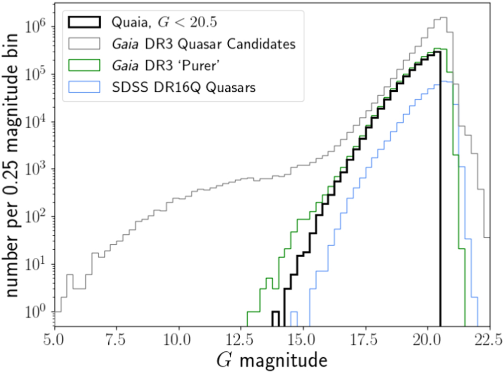
We show the G-band magnitude distribution of Quaia in Figure 12, in comparison to the other Gaia and SDSS quasar samples described above. We see that our catalog (as well as the Gaia DR3 purer sample) has removed all of the sources with excessively bright (for quasars) magnitudes G < 12.5 that are present in the full Gaia sample, as well as many sources with 12.5 < G < 16. For the Gaia DR3 and SDSS samples, the number of quasars drops off sharply after G ∼ 20.75; to avoid the complicated selection effects at these depths, we limit our catalog to G < 20.5 as shown. We also note that the SDSS DR16 quasars do not extend as bright as Quaia, and this extrapolation past the training set could bias the results in this regime, though in practice this affects very few sources.

Zoom In Zoom Out Reset image size

We note that some of the Quaia sources may technically be considered lower-luminosity AGNs, or Seyfert-like galaxies, rather than quasars. We estimate the fraction of these sources using the criterion of Schneider et al. (2010): sources are considered true quasars if they have SDSS i-band luminosity M_i brighter than M_i = −22.0. To estimate the i-band magnitude for our Gaia sources, we compute the median G − i color for the subset of Quaia sources with SDSS crossmatches, where G is the Gaia G band, and then subtract this value from the G-band magnitudes to obtain an effective i-band magnitude for all Quaia sources. We convert these to absolute magnitudes M_i assuming a flat ΛCDM cosmology with H₀ = 70 km s⁻¹ Mpc⁻¹, Ω_m = 0.3, and Ω_Λ = 0.7, following Schneider et al. (2010), and assuming a value of dust reddening of A_v /E(B − V) = 1.698 corresponding to the SDSS i band and R_v = 3.1. We find that a small fraction, 8%, of Quaia sources have effective M_i < −22.0 and thus do not meet this standard luminosity criterion for being true quasars. This distinction may be important for certain studies, though may not be relevant for others, and should be kept in mind for analyses of Quaia.

We show the results of our selection function modeling (Section 3.3) for the G < 20.0 catalog in Figure 13. The selection function map is shown in Figure 13(a), where the values are the relative completeness; note that these should not be interpreted as a probability, and users may choose to normalize these values in different ways. The relationship of the selection function model to the dust and source density maps is clear visually. In Figure 13(b), we show the fractional residuals between a random catalog downsampled by this selection function and the true quasar catalog. The residuals generally look like homogeneous noise, indicating a good fit; the root mean squared fractional error is 0.49.

Zoom In Zoom Out Reset image size

Around the edges of the Galactic plane the residuals show a slight bias to positive values (meaning the completeness there was predicted to be higher than it actually is); in the region around zero Galactic longitude just above the Galactic plane, the residuals are slightly biased to negative values (meaning the completeness there was predicted to be lower than it is). These discrepancies indicate that our templates are not fully capturing the selection effects in these regions. As these are largely limited to the region around the Galactic plane, the issue could be circumvented by applying a latitude cut for sensitive analyses. The underdensity around the LMC is well modeled by the selection function, with no clear residual in that region. The selection function map for the G < 20.5 catalog (not shown) is similar with some moderate differences, and is also provided as a data product.

The selection function may change more significantly for different subsets of the catalog, such as redshift bins. The selection function should be refit for a given sample to be analyzed; we provide a code to fit the selection function for any other subset of the catalog. We note that depending on the subsample, certain regions may be more poorly modeled, and in particular, the regions around the LMC and SMC; users should check the residuals and may choose to mask the regions around the LMC and SMC to be more conservative.

We compare Quaia to other existing quasar catalogs: Projections of these catalogs are shown in Figure 14. We show the Gaia DR3 purer sample (Figure 14(a)); a crossmatched catalog of WISE and Pan-STARRS (WISE-PS1), a current leading large-area photometric redshift quasar sample (Figure 14(b)); the SDSS DR16Q catalog, the current best spectroscopic sample of quasars (Figure 14(c)); the eBOSS quasar clustering catalog, the subsample of SDSS DR16Q intended for clustering analyses (Figure 14(d)); and Milliquas, a meta-catalog compiling confirmed quasars from the literature (Figure 14(e)).

Zoom In Zoom Out Reset image size

The Gaia DR3 purer sample is described in Section 2.1; here we include only sources with QSOC redshift estimates (z_Gaia). The WISE-PS1 sample was constructed by Beck et al. (2022), based on the Source Types and Redshifts with Machine learning (STRM) algorithm by Beck et al. (2020). The quasar catalog with updated photometric redshifts is presented by Kunsági-Máté et al. (2022); here we include only those quasars with redshifts labeled reliable, which is 59% of the sample. The SDSS DR16Q quasar catalog is the one described in Section 2.3, from Lyke et al. (2020), which compiles sources from eBOSS as well as previous SDSS campaigns (and is intended as a superset of SDSS quasars rather than a uniform sample). The eBOSS quasar clustering catalog is detailed in Ross et al. (2020); it is a subsample of SDSS DR16Q selected for large-scale structure clustering analyses, and as such is much more homogeneous than the full catalog. For the eBOSS clustering catalog, we have included both eBOSS and legacy SDSS quasars (IMATCH = 1 or 2) and applied the clustering cuts of requiring sectors to have >0.5 completeness (COMP_BOSS) and redshift success rate (sector_SSR); we have additionally removed sources with ZWARNING! = 0. The Milliquas catalog was compiled by Flesch (2021); a significant portion of the sources are from SDSS and AllWISE. For each of these samples, we have shown quasars brighter than a limiting magnitude of G ∼ 20.5; for the non-Gaia catalogs we convert to G from the survey's r-band magnitude using the conversion in Equation (2) of Proft & Wambsganss (2015), which is based on the SDSS $r^{\prime}$ band. While this should give a reasonable estimate for the SDSS sample (using r_SDSS) and the WISE-PS1 sample (using r_PS1 which is very similar to r_SDSS), it may not be as reliable for Milliquas which catalogs red magnitudes from various sources, as well as for sources with z > 3, which were not included in the Proft & Wambsganss (2015) fit.

A summary of the catalogs is shown in Table 1, for the full catalogs (limited to sources with reliable redshifts) as well as the G_eff < 20.5 subsamples. We exclude Milliquas from this comparison given its very heterogeneous nature; we do include SDSS DR16Q, though it is also not intended to be uniform, to show the comparison of Quaia to this large spectroscopic catalog of quasars. For these quantifications, we exclude areas that have A_V > 0.5 mag, as well as healpixels with no quasars. For the sky fraction f_sky, we see that Quaia and Gaia DR3 purer are limited only by the dusty regions, and cover over 30% more area than WISE-PS1 (which is limited by Pan-STARRS), nearly three times that of SDSS DR16Q, and over five times that of the eBOSS quasar clustering catalog. Compared to the Gaia DR3 purer sample, Quaia has a slightly smaller number of sources, but due to its redshift distribution gives a slightly higher effective volume. The on-sky number density is similar for all of the catalogs when limiting them to similar magnitudes, with WISE-PS1 slightly higher because it has a similar number of objects to the Gaia catalogs but over a smaller area, and SDSS DR16Q and the eBOSS clustering catalog slightly lower. When including faint sources for the catalogs, WISE-PS1 has two and a half times the on-sky number density as Quaia, and SDSS DR16Q and the eBOSS clustering catalog have one and a half to two times.

Table 1. Comparison between Quaia and Other Existing Quasar Catalogs, Detailed in the Text

	N	fsky	$\bar{n},{\deg }^{-2}$	${V}_{\mathrm{span}},{({h}^{-1}\,\mathrm{Gpc})}^{3}$	${V}_{\mathrm{eff}},{({h}^{-1}\,\mathrm{Gpc})}^{3}$	zmed	f(∣δ z∣ < 0.01)	f(∣δ z∣ < 0.1)
Quaia	1,234,715	0.73	40.78	143.78	7.08	1.48	0.63	0.84
Gaia purer	1,647,311	0.73	54.42	143.76	9.24	1.63	0.53	0.62
G < 20.5	1,286,788	0.73	42.51	143.76	6.50	1.61	0.62	0.70
WISE-PS1	2,386,121	0.56	103.89	109.08	20.88	1.38	0.11	0.71
Geff < 20.5	1,130,925	0.56	49.25	109.06	7.32	1.41	0.12	0.76
SDSS DR16Q	637,371	0.26	60.18	50.30	4.16	1.77	∼1	∼1
Geff < 20.5	297,940	0.26	28.17	50.23	1.18	1.67	∼1	∼1
eBOSS clustering	409,286	0.14	72.52	26.80	3.21	1.60	∼1	∼1
Geff < 20.5	190,263	0.14	33.96	26.61	1.01	1.49	∼1	∼1

Note. We show the quantities for the full catalogs (for sources with reliable redshifts) as well as the catalogs limited to G < 20.5 or the rough equivalent converted from another band. For all quantities and catalogs shown, we exclude areas with high dust extinction (A_V > 0.5 mag); this excludes ∼5% of sources for Quaia and Gaia DR3 purer, ∼18% of the full WISE-PS1 sample, and a negligible number of sources for SDSS DR16Q and the eBOSS clustering catalog. We note that the SDSS DR16Q catalog is a superset of quasars from many SDSS campaigns and is not intended to be uniform, which should be considered in particular for the sky fraction and spanning volume quantities. We show the number of sources N, the fraction of sky area covered f_sky, the mean number density per square degree $\bar{n}$, the spanning volume between 0.8 < z < 2.2 V_span, the effective volume V_eff, the median redshift z_med, and the fraction of objects with ∣δ z∣ ≡ ∣Δz/(1 + z)∣ < 0.01 and <0.1 (where applicable).

Download table as:  ASCIITypeset image

For the volume comparison, we compute two different volumes. The first is a simple spanning volume, V_span, which is just the comoving volume in the sky area of the survey (as given by f_sky of the full sky area) in a redshift range 0.8 < z < 2.2, a typical redshift range for clustering analyses (taken from the range of the eBOSS quasar clustering catalog). Thus, it compares in the same way as the survey areas, but gives an idea of the physical volume the catalogs span. The second is the effective volume, described in Section 4.1; we use that same $P{(k)=4\times {10}^{4}\ ({h}^{-1}\,\mathrm{Mpc})}^{3}$ for the volume calculation for all catalogs. We see that the effective volume of WISE-PS1 is much larger (nearly three times) than that of Quaia as a result of its larger number of sources, though when considering samples with the same limiting magnitude, WISE-PS1 and Quaia have comparable effective volumes. The effective volume of Quaia is nearly twice as large as that of SDSS DR16Q, and 6× for the magnitude-limited sample; compared to the eBOSS quasar clustering catalog, the effective volume of Quaia is over twice as large, and 7× for the magnitude-limited sample.

The catalogs all have a similar median redshift, of around 1.4 < z < 1.7, extending to 1.77 for SDSS DR16Q when including faint sources. However, they have significantly different redshift precision; in Table 1 we show outlier fractions estimated from comparisons to spectroscopic redshifts. We see that both of the Gaia catalogs have a similar fraction of high-precision redshifts (∣Δz/(1 + z)∣ < 0.01), but Quaia has a much higher fraction of redshifts that are not strong outliers (∣Δz/(1 + z)∣ < 0.1) compared to Gaia DR3 purer. WISE-PS1 falls between Quaia and Gaia DR3 purer in terms of strong outliers, but has an extremely low fraction of high-precision redshifts as it is a photometric survey. We note that for both Gaia DR3 purer and WISE-PS1, the redshift precision is significantly lower when considering the full catalog compared to samples limited to G_eff < 20.5 like Quaia; we show both for a fair comparison. The SDSS DR16Q catalog and the eBOSS quasar clustering catalog have spectroscopic redshifts, so these are almost all very high precision; Lyke et al. (2020) estimated from a visual inspection that less than 1% of the SDSS DR16Q redshifts are outliers with Δv > 3000 km s⁻¹ (∣Δz∣ > 0.01), independent of redshift; note that this is a slightly different sample than the eBOSS clustering catalog, but we can expect it to be similar. The SDSS DR16Q quasar sample has typical statistical redshift errors of ∣Δz∣ ∼ 0.001.

To give more of an idea of the redshift precision of Quaia, we compare it to existing all-sky photometric galaxy catalogs. A common statistic to summarize photometric redshift uncertainty robust to outliers is the SMAD, scaled median absolute deviation, defined as 1.4826 × med(∣Δz − med(Δz)∣), where Δz = z_phot − z_spec (the scaling factor adjusts the MAD such that SMAD is approximately equal to the standard deviation for normalized data). The SMAD of the full Quaia catalog (G < 20.5) is SMAD(Δz) = 0.023, and the normalized SMAD of the redshift errors with the (1 + z) factor divided out is SMAD(Δz/(1 + z)) = 0.008. For comparison, the WISE × SuperCOSMOS catalog of 20 million galaxies with z_med = 0.2 (Bilicki et al. 2016) has an SMAD(Δz) of ∼ 0.04 and an SMAD(Δz/(1 + z)) of ∼ 0.035. The Two Micron All Sky Survey Photometric Redshift (2MPZ) catalog has around 1 million galaxies with a similar median redshift (Bilicki et al. 2013), which have an SMAD (Δz) of ∼ 0.015. Quaia thus falls in between these common photometric galaxy samples in terms of overall redshift precision; however, we note that it is difficult to capture the redshift error of Quaia in a single statistic, given both its large number of highly precise redshifts and non-insignificant number of outliers.

We also note that the ongoing DESI survey (Aghamousa et al. 2023; DESI Collaboration et al. 2024) will observe a high density of quasars over a large sky area (Chaussidon et al. 2023), which will be competitive with and complementary to Quaia.

The complete Quaia catalog contains our decontaminated quasar sample with computed redshift information, relevant Gaia properties, and crossmatched catalog information. The complete catalog format with column names, units, column descriptions, and an example entry is shown in Table 2. Additional information for the sources can be obtained by joining the catalog with the relevant data source with the associated identifier (Gaia or unWISE). We include only sources with G < 20.5 in the catalog; we also publish a version limited to G < 20.0, along with the selection function models fit to each (Section 4.2) and random catalogs generated from the selection functions. The catalog includes our SPZ redshifts z_Gaia along with 1σ redshift errors, sky position, Gaia photometry, unWISE photometry, and proper motion information. The catalog is in FITS format (Wells et al. 1981), and units and descriptions are provided for each column.

Table 2. Format and Column Descriptions of Quaia, Published as a FITS Data File (Wells et al. 1981)

Column Name	Symbol	Units	Description	Example Entry Value
source_id	⋯	⋯	Gaia DR3 source identifier	6459630980096
unwise_objid	⋯	⋯	unWISE DR1 source identifier	0453p000o0014479
redshift_quaia	zQuaia	⋯	Spectrophotometric redshift estimate	0.416867
redshift_quaia_err	⋯	⋯	1σ uncertainty on spectrophotometric redshift estimate	0.060812
ra	⋯	deg	Barycentric R.A. of the source in ICRS at 2016.0	44.910498
dec	⋯	deg	Barycentric decl. δ of the source in ICRS at 2016.0	0.189649
l	⋯	deg	Galactic longitude	176.659434
b	⋯	deg	Galactic latitude	−48.835164
phot_g_mean_mag	G	mag	Gaia G-band mean magnitude	20.173105
phot_bp_mean_mag	BP	mag	Gaia integrated BP mean magnitude	20.200150
phot_rp_mean_mag	RP	mag	Gaia integrated RP mean magnitude	18.871586
mag_w1_vg	W1	mag	unWISE W1 magnitude	14.774343
mag_w2_vg	W2	mag	unWISE W2 magnitude	13.923867
pm	μ	mas yr−1	Total proper motion	0.383797
pmra	μα*	mas yr−1	Proper motion in R.A. ${\mu }_{\alpha * }\equiv {\mu }_{\alpha }\,\cos \,\delta$ of the source in ICRS at 2016.0	0.217806
pmdec	μδ	mas yr−1	Proper motion in decl. μδ of the source in ICRS at 2016.0	−0.316007
pmra_error	σμ α*	mas yr−1	Standard error of proper motion in R.A. direction	0.679419
pmdec_error	σμ δ	mas yr−1	Standard error of proper motion in decl. direction	0.608799

Note. For an example entry, we show the first catalog row.

Download table as:  ASCIITypeset image

While the Quaia catalog presents a highly useful quasar sample, it does have various limitations. We reiterate and discuss the main ones here.

We estimate spectrophotometric redshifts for the quasars, which are generally more accurate than the Gaia estimates, but are still low precision compared to spectroscopic redshifts. The uncertainties on these redshifts should be taken into account for any measurements, and the rate of catastrophic redshift errors (not necessarily captured by the redshift uncertainty) should be considered when thinking about possible uses of the catalog.

The selection function model has multiple potential limitations. While it broadly captures the selection effects that affect the quasar sample, it has significantly lower accuracy around the galactic plane; precision measurements may require masking this region. The regions around the LMC and SMC are also more poorly modeled; users may want to mask this area. We also note that we are not fitting the healpixels with zero quasars, which may result in a slight bias toward populated regions, and fixes the zero-probability region of the selection function. Our selection function map depends only on-sky position and not other properties such as magnitude or redshift (besides fitting it to the appropriate subsample); a treatment incorporating these dependencies may be important for certain uses. The gold standard for completeness estimation is data injection and recovery tests. Unfortunately, the Gaia instrumentation has black-box elements, such as onboard image segmentation, onboard object detection, and onboard downlink prioritization, that make it impossible to perform end-to-end injection tests, so we rely on a data-driven approach, which may be less robust and more sensitive to modeling choices. Given this, it is possible that we are overfitting the selection function. Finally, the selection function depends on the assumption of isotropy, which we know to be broken to some extent by the kinematic dipole (Stewart & Sciama 1967; Secrest et al. 2021); we will explore and measure this in an upcoming work (see Section 4.6). Users employing the selection maps or generating their own selection function for some subset of the catalog should take note of these potential issues.

Generally, Quaia has a relatively low number density (e.g., compared to the SDSS sample). This means that it may not be ideal for certain cosmological measurements, which may be shot noise dominated.

Finally, we note that this catalog is based on the Gaia quasar candidates sample, and it will inherit many of the limitations of that sample (Gaia Collaboration et al. 2023a). We are also limited to the Gaia-derived properties (e.g., the Gaia redshifts that are a feature for our estimates). In upcoming Gaia data releases, the collaboration will release more BP/RP spectra and we will have the opportunity to work directly from the spectral data to improve the catalog.

Quasars are highly biased tracers of the cosmic web that trace the matter distribution at higher redshift than galaxies and in the mildly nonlinear regime. Given the Quaia catalog's sampling of quasars to deep magnitudes and across a large volume, and its reduced systematic contamination allowed by space-based observations, Quaia lends itself to large-scale structure analyses, many of which are currently ongoing.

Thanks to its large volume and well-characterized selection function, Quaia is perhaps the best current sample for testing homogeneity and isotropy in the Universe (D. W. Hogg et al. 2024, in preparation), and relatedly for measuring the dipole in the quasar distribution (A. Williams et al. 2024, in preparation), which recent measurements have consistently found to be in mild tension with the kinematic interpretation in the ΛCDM model. Quaia's volume also makes it a good sample for a measurement of the matter-radiation equality scale, k_eq (e.g., Bahr-Kalus et al. 2023).

The catalog is particularly well suited for cross-correlations with other all-sky observations of projected tracers of the large-scale structure, which are less sensitive to redshift errors compared to 3D ones. Examples of this are the CMB, the CIB, or maps of the thermal Sunyaev–Zel'dovich effect. Aghamousa et al. (2023) used the cross-correlation between CMB lensing and Quaia to constrain the growth of matter fluctuations via the parameter S8, achieving competitive constraints as well as showing that Quaia can break the degeneracy between Ω_m and σ₈. An analysis of primordial non-Gaussianity (parameterized by f_NL) from this cross-correlation with CMB lensing is also underway. Analyses of the cross-correlation with CMB temperature to measure the Integrated Sachs–Wolfe effect, and with the CIB to constrain the star formation history at high redshifts (e.g., Jego et al. 2023), are currently under investigation. Another measurement enabled by the catalog is the cross-correlation of quasar proper motions with the large-scale structure, which directly estimates the cosmological quantity Hf σ₈ (Duncan et al. 2024). Additionally, cross-correlations of Quaia with galaxy surveys may allow for measurements of the baryon acoustic feature (Patej & Eisenstein 2018; Zarrouk et al. 2021) and quasar environments (Padmanabhan et al. 2009; Shen et al. 2013).

Quaia is also useful for void studies, including constraining core cosmological parameters with the void size distribution; this investigation is underway (N. Arsenov et al. 2024, in preparation). The catalog is additionally relevant to astrophysical analyses of quasar properties, given its large sky coverage and multiband photometry, such as the role of galaxy interactions on AGN activity. Quaia sources may also be used to study the potential of quasars as standard candles. Further, Quaia provides perhaps the best quasar coverage of the southern sky, which may be important for a variety of applications such as identifying interesting sources there, adding new information to known sources, or calibrating surveys in that sky region. Finally, while a 3D clustering analysis of Quaia may be limited by the catalog's relatively low number density and moderate redshift precision, a careful analysis may yield useful constraints, especially using techniques targeted at wide-field surveys (e.g., Lanusse et al. 2015).

The latter is comparable or better than other state-of-the-art galaxy and quasar samples used in large-scale structure analyses, but not enough to necessarily allow an accurate interpretation.