


Abstract
A gravitational anomaly is found at weak gravitational acceleration gN ≲ 10−9 m s−2 from analyses of the dynamics of wide binary stars selected from the Gaia DR3 database that have accurate distances, proper motions, and reliably inferred stellar masses. Implicit high-order multiplicities are required and the multiplicity fraction is calibrated so that binary internal motions agree statistically with Newtonian dynamics at a high enough acceleration of ≈10−8 m s−2. The observed sky-projected motions and separation are deprojected to the 3D relative velocity v and separation r through a Monte Carlo method, and a statistical relation between the Newtonian acceleration gN ≡ GM/r2 (where M is the total mass of the binary system) and a kinematic acceleration g ≡ v2/r is compared with the corresponding relation predicted by Newtonian dynamics. The empirical acceleration relation at ≲10−9 m s−2 systematically deviates from the Newtonian expectation. A gravitational anomaly parameter δobs−newt between the observed acceleration at gN and the Newtonian prediction is measured to be: δobs−newt = 0.034 ± 0.007 and 0.109 ± 0.013 at gN ≈ 10−8.91 and 10−10.15 m s−2, from the main sample of 26,615 wide binaries within 200 pc. These two deviations in the same direction represent a 10σ significance. The deviation represents a direct evidence for the breakdown of standard gravity at weak acceleration. At gN = 10−10.15 m s−2, the observed to Newton-predicted acceleration ratio is  . This systematic deviation agrees with the boost factor that the AQUAL theory predicts for kinematic accelerations in circular orbits under the Galactic external field.
Export citation and abstract BibTeX RIS

Original content from this work may be used under the terms of the Creative Commons Attribution 4.0 licence. Any further distribution of this work must maintain attribution to the author(s) and the title of the work, journal citation and DOI.
1. Introduction
General relativity is the standard relativistic theory of gravity with its nonrelativistic limit matching Newton's inverse square law of gravitational force, or Poisson's equation. The standard Newton–Einstein theory satisfies the strong equivalence principle (Will (2014)) and does not permit any external field effect (Milgrom 1983a) in internal dynamics of a self-gravitating system falling freely under a uniform external field.
The observed deviation of the internal kinematics of galaxies and galaxy clusters from the Newtonian prediction is usually attributed to unidentified dark matter (DM). This has been the most popular interpretation of the astronomical data backed by the "right" amount of DM in the universe inferred from the standard cosmology based on general relativity (Peebles 2022).
Alternatively, the observational fact that nonrelativistic dynamics of galaxies already exhibits kinematic deviation may indicate that even Newtonian dynamics may need to be modified, as first suggested by Milgrom (1983a, 1983b). Modified Newtonian dynamics (MOND) has been theorized as modified Poisson's equations (Bekenstein & Milgrom 1984; Milgrom 2010) or modified inertia (Milgrom 1994, 2022), breaking the strong equivalence principle (keeping, however, the experimentally better tested Einstein equivalence principle) and following Mach's principle in spirit. It is possible to distinguish with astronomical data the theoretical predictions of modified gravity (modified Poisson's equations), modified inertia, and the standard theory assuming DM. A recent study (Chae 2022) with galactic rotation curves indicates that modified gravity represented by the AQUAL (A-QUAdratic Lagrangian) theory (Bekenstein & Milgrom 1984) is preferred over modified inertia and the standard theory. In addition, Chae et al. (2022) showed that AQUAL is somewhat preferred over another Lagrangian theory of modified gravity called quasi-linear MOND (Milgrom 2010). Stronger tests with larger and better data of galactic rotation curves are expected in the future.
For the past decade, binary stars have been considered (e.g., Hernandez et al. 2012; Banik & Zhao 2018; Pittordis & Sutherland 2018; El-Badry 2019; Hernandez et al. 2019; Pittordis & Sutherland 2019; Clarke 2020; Hernandez et al. 2022; Hernandez 2023; Pittordis & Sutherland 2023) as a potentially powerful tool to test gravity at weak acceleration ≲10−10 m s−2 when two stars are separated widely enough, typically more than several kilo–astronomical units (kau). Testing gravity with wide binaries is interesting because DM can play no role in their internal dynamics. Thus, unlike galaxies and galaxy clusters, there is no need to distinguish predictions of modified gravity and DM that appear to overlap and differ only subtly in some cases.
However, unlike the galactic rotation curve in a disk galaxy where motions of particles can be well described by circular orbits in an orbital plane of a measurable inclination, it is not straightforward to interpret the observed proper motions (PMs), i.e., sky-projected 2D motions, of wide binaries, because orbits are highly eccentric, and individual inclinations are unknown. The projection or perspective effect needs to be taken into account to properly interpret the observed 2D motions (e.g., El-Badry 2019; Pittordis & Sutherland 2023).
Moreover, all relevant astrophysics of wide binaries needs to be properly taken into account to test gravity. One of the most important factors is the statistics and property of stellar multiplicity (Duchêne & Kraus 2013). In any sample of wide binaries, no matter how the sample is selected from the currently available databases, it is inevitable for some binaries to hide close inner companions (e.g., Belokurov et al. 2020; Penoyre et al. 2022). In other words, some fraction of apparent wide binaries are actually triples or quadruples (or even higher multiples in rare cases). The hidden inner companions have been a source of much uncertainty (Clarke 2020) in recent wide binary tests.
Another crucial factor that is illustrated in detail in this work is the eccentricity distribution in wide binaries that is varying with the separation or period of the system. Additionally, as we will be shown, the measurement uncertainties of PMs pose a concern in testing gravity for wide binaries at distances larger than about 100 pc, even for recent Gaia Early Data Release 3 (EDR3; Brown et al. 2021) and DR3 (Vallenari et al. 2023) databases. 1
In this paper, we carry out a new analysis of nearby wide binaries (El-Badry et al. 2021) selected from a Gaia DR3 database, taking into account the projection effect and undetected inner companions and examining the effects of larger data uncertainties at larger distances. To circumvent the projection effects, we consider a Monte Carlo (MC) deprojection of the observed 2D motions to 3D motions and work with MC-realized 3D relative velocity v and 3D separation r. We then compare statistically the resulting MC set of accelerations with a corresponding Newtonian MC set expected by Newtonian dynamics in an acceleration plane. We define a deviation in the acceleration plane δobs−newt and compare its value with the null prediction (δobs−newt = 0) and the AQUAL prediction (δobs−newt > 0 at acceleration ≲10−9 m s−2) that systematically varies with acceleration. In this test, not only can Newton's prediction be tested robustly but also Newton's and modified gravity theories can be discriminated in a straightforward and generic way.
As for samples of wide binaries, we first define a nearby benchmark sample within a distance of 80 pc that have accurate PMs and all other well-measured quantities. For most wide binaries in the benchmark sample, the Gaia DR3-reported measurement errors of PMs are automatically < 1%. We then consider wide binaries up to 200 pc, but use only those that satisfy the precision of PMs of the benchmark sample. It is found that these accurate PMs reveal an immovable anomaly of gravity in favor of MOND-based modified gravity.
The contents of this paper are as follows. Section 2 describes the samples of wide binaries and the observational inputs that are needed. Section 3 describes the method of modeling and statistical analyses. In detail, Section 3.1 describes how 2D motions are deprojected to 3D motions allowing all possibilities within observational constraints. Section 3.2 describes how undetected close companions are modeled, while Section 3.3 describes how deprojected MC sets are analyzed in the acceleration plane. Section 3.4 describes how virtual wide binaries for the Newtonian ensemble are obtained in a universe obeying the Newton–Einstein gravity, and Section 3.5 provides a description of a pseudo-Newtonian simulation. In Section 4, we present the results. We first validate the whole methodology by carrying out the analysis with realistically produced mock wide binaries in a universe obeying Newtonian dynamics (Section 4.1), and present the main (Section 4.2) and alternative results (Sections 4.3). In Section 5, we compare our results with the most relevant previous and concurrent tests of gravity with wide binaries, speculate any possible systematic that could remove the gravitational anomaly, and discuss theoretical implications of the anomaly. In Section 6, we summarize the conclusions and discuss future prospects for further tests of gravity with wide binaries. In Appendix A, the effects of binning in an acceleration plane are discussed. In Appendix B, the effects of PM errors are explored. In Appendix C, the effects of eccentricities are illustrated with a biased eccentricity distribution. Wide binary samples and Python scripts used in modeling and statistical analyses can be accessed at Zenodo: doi:10.5281/zenodo.8065875.
2. Data and Observational Inputs
2.1. Wide Binary Sample
Starting with a large catalog of over 1 million binaries within ≈1 kpc (El-Badry et al. 2021) derived from Gaia EDR3 (Brown et al. 2021), we intend to select a sample best-suited to test gravity. Testing gravity with wide binaries requires accurate measurements of three key quantities: PMs, distances, and masses. Because this study is designed to test gravity theories that may deviate from standard gravity at weak acceleration, masses cannot be determined from the observed kinematics assuming Newtonian dynamics for systems with separation greater than several kau. Thus, masses must be determined from photometric observations with an empirical mass–magnitude relation.
Gaia provides measurements of PMs as well as parallaxes and G-band magnitudes, from which distances and absolute magnitudes are determined. Because parallaxes and PMs are measured geometrically, their measurement uncertainties increase with distance (see below). Photometric measurements also become less accurate with distance because stars become fainter and dust extinction becomes nonnegligible (see below). Thus, nearby wide binaries provide the most accurate and reliable data for gravity test. However, because nearby wide binaries are relatively few, statistical uncertainties may be a concern when a decisive (e.g., well beyond conventional 5σ significance) test of gravity is desired. On the other hand, data selection needs to be done carefully in using more distant wide binaries because data qualities can be a concern for them.
We first define relatively small benchmark nearby samples of good qualities within 80 pc, and then use the benchmark data qualities in defining larger samples at larger distances. We consider up to 200 pc for reasons mentioned below.
The benchmark distance of 80 pc is chosen for several reasons. First, most PMs have a precision of 1% or better within this distance. Second, we consider binaries with relatively small projected separation (s) down to 200 au as calibration systems for which Newtonian dynamics must hold. For s > 200 au, distance limit d < 80 pc insures that two stars are separated by more than 2 5 on the sky, which insures that photometric measurements of both stars are reliable. Third, for d < 80 pc, dust extinction is negligible (see below). Fourth, a similar distance limit of d < 67 pc has been considered in some binary observational programs to study multiplicity (Tokovinin 2014a,2014b; Riddle et al. 2015). High-order multiplicity plays a decisive role in wide binary tests, as hidden close companions provide additional gravitational forces. Because our distance limit is similar to that defined by these observations, we may use their results as an input or guidance for our study. Finally, El-Badry et al. (2021) excluded systems with resolved additional components in constructing their binary sample. This means that all binaries in the El-Badry et al. (2021) sample do not have detectable (G ≲ 21) tertiary (and additional) components separated more than 1'' from the binary components. Then, all binaries with d < 80 pc from El-Badry et al. (2021) are free of resolved additional stars up to the limit MG
≈ 16.5, which is several magnitudes fainter than the observed stars of typical binaries.
5 on the sky, which insures that photometric measurements of both stars are reliable. Third, for d < 80 pc, dust extinction is negligible (see below). Fourth, a similar distance limit of d < 67 pc has been considered in some binary observational programs to study multiplicity (Tokovinin 2014a,2014b; Riddle et al. 2015). High-order multiplicity plays a decisive role in wide binary tests, as hidden close companions provide additional gravitational forces. Because our distance limit is similar to that defined by these observations, we may use their results as an input or guidance for our study. Finally, El-Badry et al. (2021) excluded systems with resolved additional components in constructing their binary sample. This means that all binaries in the El-Badry et al. (2021) sample do not have detectable (G ≲ 21) tertiary (and additional) components separated more than 1'' from the binary components. Then, all binaries with d < 80 pc from El-Badry et al. (2021) are free of resolved additional stars up to the limit MG
≈ 16.5, which is several magnitudes fainter than the observed stars of typical binaries.
The statistical sample within 80 pc is defined based on the following selection criteria. For each binary system, the brighter (primary) and fainter (secondary) stars are referred to as components A and B, respectively.
- 1.Both stars belong to the main sequence (the binary type is "MSMS" according to the definition by El-Badry et al. 2021).
- 2.
- 3.
 (distances of two components agree within 3σ).
 - 4.Relative errors of PM components for each binary are all smaller than 0.01 (or 0.005 as an alternative choice). Median ruwe value for the selected stars is 1.03.
- 5.The sky-projected separation is in the range 0.2 < s < 30 kau.
- 6.Absolute magnitudes for both components are within a "clean range" 4 < MG < 14 or a "strict range" 4 < MG < 12.


Figure 1 shows the clean and strict samples within 80 pc in a color–magnitude diagram. As shown in the upper panels, the magnitude cut 4 < MG < 14 for the clean sample excludes some bright main-sequence and giant stars as well as very faint stars that exhibit large scatters in the Gaia BP−RP color. When the magnitude cut is applied to both primaries and secondaries, the color scatter is significantly reduced as shown in the lower-left panel. When the stricter cut 4 < MG < 12 is applied, the color scatter is further reduced, as shown in the lower-right panel. We exclude small numbers of remaining binaries that have component(s) outside the diagonal cut line although they have essentially no impact on our studies. The clean and strict samples have, respectively, 4077 and 3170 binaries, both of which include hundreds of widely (4 ≲ s < 30 kau) separated binaries in a low acceleration regime ≲10−10 m s−2.

Figure 1. A color–magnitude diagram for wide binaries within 80 pc is shown for primaries (the brighter components) and secondaries. MG is the Gaia DR3 G-band absolute magnitudes with distances from parallaxes, and BP−RP is a Gaia DR3 color. The clean and strict samples are indicated by color bands of the MG ranges. As shown in the bottom panels, when the MG ranges are applied to both components, color scatters are largely removed.
Download figure:
Standard image High-resolution imageFigure 2 shows how measurement uncertainties of distances and PMs vary with distance up to dA = 200 pc. The dM < 80 pc (hereafter dM refers to the error-weighted mean of two distances of the binary components) samples (in particular, the strict sample) have relatively small uncertainties: for most binaries, both distance and PM relative uncertainties are smaller than 1% or 0.5%. All uncertainties increase with distance. Relative uncertainties of distances are not a critical factor in testing gravity because two stars in a binary system can be assumed to be in the same distance 2 compared to the small separation (≲30 kau) as long as the binary identification is correct. However, relative uncertainties of PMs are critically important because the sky-projected relative velocity magnitude between the two stars is derived from the difference between the PMs of the stars.

Figure 2. The first and second columns show relative uncertainties (taking the larger of the two uncertainties) of distances and proper motions (PMs) with respect to dM (weighted mean distance of the two components) for the clean (upper) and strict (lower) ranges of MG . The third column shows that both uncertainties are correlated. The horizontal magenta lines indicate a cut of 0.01 or 0.005 for relative errors of PMs. Data above either cut line are not used. Note that only a small fraction of binaries is removed by either cut for the samples with dM < 80 pc, while a large portion is removed for samples with larger distance limits.
Download figure:
Standard image High-resolution imageFigure 3 shows dust extinction at the G band, AG , as a function of distance and galactic latitude. We use dustmaps 3 (Green 2018; Green et al. 2019) to estimate reddening E(B − V) and use the standard formula AV = 3.1E(B − V) to estimate extinction in the Johnson-Cousins V-band. Finally, AV is transformed into AG following the recommendation on the Gaia website (Fitzpatrick et al. 2019). 4 Clearly, dust extinction is negligible for dM < 80 pc. Figure 3 reveals two points. At larger distances, dust extinction is no longer negligible, and it is not limited within a narrow galactic latitude such as ∣b∣ < 15 as often assumed in the literature (e.g., Pittordis & Sutherland2019, 2023).

Figure 3. Dust extinction (AG ) in the Gaia DR3 G band is estimated as described in the text based on the dustmaps package for decl. > − 28°. Dust extinction is estimated only for this range. The left and right panels shows AG with respect to distance and galactic latitude.
Download figure:
Standard image High-resolution imageClearly, the distance limit of 80 pc insures the good data qualities required for an accurate test. However, we also consider data at larger distances up to 200 pc with the same PM quality cut of 1% (or 0.5%) relative error (as imposed on the dM < 80 pc data). The PM quality cut removes a large portion of more uncertain data so that the remaining data are of comparable quality in relative PM precision to the benchmark data. The distance limit of 200 pc insures that two stars are separated more than 1'' for the considered separation s > 200 au to insure that they are well resolved in the Gaia DR3 photometry. The size of the dM < 200 pc sample is 6.5 times larger than the dM < 80 pc sample. The color–magnitude diagram for the dM < 200 pc sample can be found in Figure 4.

Figure 4. Same as Figure 1 but for the dM < 200 pc sample.
Download figure:
Standard image High-resolution imageThe above selection of statistical samples of wide binaries is entirely based on astrometric and photometric measurements. In particular, chance alignment (i.e., fly-by) cases are removed by requiring  (see El-Badry et al. 2021 for an extensive demonstration that their
  values can be used to remove fly-bys effectively). Gaia DR3 also provides spectroscopic measurements of radial velocities (vr
) for some fraction of stars (Katz et al. 2023). For the above dM
< 80 pc and dM
< 200 pc samples, 68% and 37% of wide binaries, respectively, have radial velocities for both components. However, measurement uncertainties of radial velocities are much larger than those of PMs and thus sky-projected (transverse) velocities (vp
). Median uncertainties of vr
are 0.83 and 1.33 km s−1 for the dM
< 80 pc and dM
< 200 pc samples while those of vp
are 0.007 and 0.046 km s−1 for which dA
and its uncertainties are used. See Figure 5 for the distributions of measured radial velocities and their uncertainties from the dM
< 200 pc sample.
values can be used to remove fly-bys effectively). Gaia DR3 also provides spectroscopic measurements of radial velocities (vr
) for some fraction of stars (Katz et al. 2023). For the above dM
< 80 pc and dM
< 200 pc samples, 68% and 37% of wide binaries, respectively, have radial velocities for both components. However, measurement uncertainties of radial velocities are much larger than those of PMs and thus sky-projected (transverse) velocities (vp
). Median uncertainties of vr
are 0.83 and 1.33 km s−1 for the dM
< 80 pc and dM
< 200 pc samples while those of vp
are 0.007 and 0.046 km s−1 for which dA
and its uncertainties are used. See Figure 5 for the distributions of measured radial velocities and their uncertainties from the dM
< 200 pc sample.

Figure 5. The top panel shows the distribution of measured radial velocities (vr ) of both components from the dM < 200 pc sample. The bottom panel shows the distribution of their uncertainties.
Download figure:
Standard image High-resolution imageAlthough typical radial velocities are not useful for testing gravity in wide binaries whose typical relative velocities between two components are < 1 km s−1, they can be used to select or test candidate binaries because for genuine binaries radial velocities of both components must match up to measurement uncertainties. The dM
< 80 pc and dM
< 200 pc samples selected with  can be tested in this regard. Figure 6 shows distributions of magnitudes of relative radial velocities between the two components from the dM
< 80 pc and dM
< 200 pc samples. The distributions of the measured values are consistent with the predicted distributions arising purely from measurement uncertainties under the hypothesis that two radial velocities are drawn from the same value of the binary system (note that the expected intrinsic differences (≲1 km s−1) between the two components are much smaller than typical random scatter of 32.6 km s−1): the observed fractions with ∣vr,A
− vr,B
∣ > 5 are nearly equal to the predicted fractions. These results reinforce the demonstration by El-Badry et al. (2021) that their
can be tested in this regard. Figure 6 shows distributions of magnitudes of relative radial velocities between the two components from the dM
< 80 pc and dM
< 200 pc samples. The distributions of the measured values are consistent with the predicted distributions arising purely from measurement uncertainties under the hypothesis that two radial velocities are drawn from the same value of the binary system (note that the expected intrinsic differences (≲1 km s−1) between the two components are much smaller than typical random scatter of 32.6 km s−1): the observed fractions with ∣vr,A
− vr,B
∣ > 5 are nearly equal to the predicted fractions. These results reinforce the demonstration by El-Badry et al. (2021) that their  values can be reliably used to select genuine binaries.

Figure 6. Distributions of the magnitudes of relative radial velocities  between the two components in wide binaries are shown for the dM
< 80 pc (left) and dM
< 200 pc (right) samples. Blue histograms represent measured values while gold histograms are the predicted distributions purely arising from measurement uncertainties under the hypothesis that the two components belong to a genuine binary system, and thus vr,A
= vr,B
up to measurement uncertainties. The observed fraction of binaries with
between the two components in wide binaries are shown for the dM
< 80 pc (left) and dM
< 200 pc (right) samples. Blue histograms represent measured values while gold histograms are the predicted distributions purely arising from measurement uncertainties under the hypothesis that the two components belong to a genuine binary system, and thus vr,A
= vr,B
up to measurement uncertainties. The observed fraction of binaries with  km s −1) denoted by f(>5 km s −1) is consistent with the Monte Carlo (MC) prediction for both samples. Note that f(>5 km s −1) is higher in the dM
< 200 pc sample due to larger measurement uncertainties at larger distances.
km s −1) denoted by f(>5 km s −1) is consistent with the Monte Carlo (MC) prediction for both samples. Note that f(>5 km s −1) is higher in the dM
< 200 pc sample due to larger measurement uncertainties at larger distances.
Download figure:
Standard image High-resolution image2.2. Mass–Magnitude Relation
Masses of both components in a binary system are estimated from their G-band magnitudes (corrected for dust extinction for stars at >80 pc). We consider mass–magnitude relations determined for nearby stars by Pecaut & Mamajek (2013) and Mann et al. (2019). Pecaut & Mamajek (2013) provided masses, several colors, and magnitudes in various wave bands for a wide range of spectral types fully covering our selected stars. Their tabulated quantities are updated on a website that is provided by E. Mamajek. 5 Additionally, Mann et al. (2019) provide accurate masses in the range 0.075 < M⋆ < 0.70M⊙ based on orbital motions of binary stars separated closely enough that significant fractions of orbits were observed, and Newtonian dynamics was used to infer accurate masses. When the Mann et al. (2019) mass–magnitude relation in the Two Micron All Sky Survey (2MASS) KS band is compared with that by Pecaut & Mamajek (2013) for the same magnitude range in the KS band, the two relations match excellently. Thus, it is sufficient to use only the tabulated quantities provided by Pecaut & Mamajek (2013).
Since Pecaut & Mamajek (2013) do not provide magnitudes in the EDR3 G-band (although they do in the DR2 G band), we transform magnitudes in other bands to the EDR3 G band. We consider two options. The first option is to transform V magnitudes to G magnitudes using the transformation provided by the Gaia collaboration (Riello et al. 2021, see their table C.2)

where XVI ≡ V − IC . The second option is to use 2MASS J-band magnitudes using

where XBR ≡ BP − RP. 6 Equation (1) has a scatter of 0.0272, and Equation (2) has a larger scatter of 0.04762. Figure 7 shows the derived relations based on the Pecaut & Mamajek (2013) MV and MJ magnitudes. The two relations differ up to 0.05 dex in mass for the relevant magnitude range considered in this study. This difference can lead to a difference in the self-calibrated multiplicity fraction, so we will consider these two relations. The polynomial-fit coefficients for the relations can be found in Table 1.

Figure 7. A couple of mass–(absolute)-magnitude relations in the Gaia EDR3 G band are derived as described in the text based on the relations given by Pecaut & Mamajek (2013) for the Johnson-Cousins V-band and 2MASS J-band magnitudes. Polynomial fits to the data are given as colored dashed curves, and the fitted coefficients can be found in Table 1. Gaia DR3 Apsis FLAME median masses are also shown for the available range (>0.5M⊙). A polynomial fit to the FLAME median masses is obtained by combing them with the J-band-based data for M < 0.5M⊙ (or MG > 10). A luminosity–mass power-law relation is compared with the mass–magnitude relations.
Download figure:
Standard image High-resolution imageTable 1. Mass–Magnitude(MG
) Relation Polynomial-fit Coefficients in 
| Coefficients | for MV -based MG | for MJ -based MG |
|---|---|---|
| a0 | 5.2951695081428651E − 01 | 4.5004396006609515E − 01 |
| a1 | −1.5827136745981818E − 01 | −7.5227632902604175E − 02 |
| a2 | 8.4871478522417707E − 03 | −1.6733691959840702E − 02 |
| a3 | 7.8449380571379954E − 04 | 3.2486543639338823E − 03 |
| a4 | −5.2267549153639953E − 05 | 9.7481038895336188E − 06 |
| a5 | −1.6957228195696253E − 05 | −3.7585795718404064E − 05 |
| a6 | 1.6858627515537989E − 06 | 2.1882376017987368E − 06 |
| a7 | −6.8083605428022648E − 08 | −2.6298611913795649E − 08 |
| a8 | 1.4781005839376326E − 09 | 1.3151945936755533E − 09 |
| a9 | 7.7057036188153745E − 11 | −9.3661053655257917E − 11 |
| a10 | −4.4776519490406922E − 12 | 4.9792442749063264E − 13 |
Download table as: ASCIITypeset image
The MV -based and MJ -based mass–magnitude relations for low-mass stars with M ≲ M⊙ exhibit two inflection points consistent with earlier observations (e.g., Kroupa et al. 1990, 1993). This means that the mass–magnitude relation does not correspond to a power-law relation between luminosity (L) and mass (M) L ∝ Mα with a single value of α for a wide range of magnitude. However, for the range of magnitudes relevant for this study, α = 3.5 provides an approximate description of the data as shown in Figure 7. This approximate relation will be used when only an approximate relation suffices as in the case that the shift of the photocenter from the barycenter is estimated in an unresolved inner binary.
Gaia DR3 provide internally determined values of astrophysical parameters for some fractions of sources through the Astrophysical parameters inference system (Apsis; Creevey et al. 2023). Stellar astrophysical parameters from the Apsis (Fouesneau et al. 2023) include "FLAME" masses for some stars with M ≥ 0.5M⊙. Figure 7 shows that FLAME masses match well with our estimated masses, in particular the MJ -based masses, except possibly for near the edge of M ≥ 0.5M⊙. However, even near 0.5M⊙ the difference is relatively minor. Because of this overall match of FLAME masses with our masses and the limited range of FLAME masses, we will not consider them in our main analyses.
2.3. Statistics and Properties of Hierarchical Systems Reported in the Literature
High-order multiplicity (Duchêne & Kraus 2013) among wide binaries is a crucial factor in wide binary tests of gravity. It would be ideal to determine accurately the high-order multiplicity for a chosen sample of wide binaries and use it as a fixed input in forward modeling of wide binary kinematics. Here we gather observational results in the literature that are most relevant for our samples.
Multiplicity varies as stellar type and mass vary. High-order multiplicity increases dramatically for early-type (O and B) stars compared to the solar type (Moe & Di Stefano 2017). However, our clean sample covers a mass range of M⋆ ≲ 1.2M⊙ (Figure 7). Thus, multiplicity among solar and subsolar types is needed for this study.
For F- and G-dwarf stars within 67 pc (Tokovinin 2014a) relevant for relatively higher-mass stars in our samples, two observational studies report measurements on the higher-order multiplicity fraction 7 among wide binaries: 0.13/0.48 = 0.28 (Figure 13 of Tokovinin 2014b) and 100/212 = 0.47 (Figure 6 of Riddle et al. 2015). For solar-type stars, Moe & Di Stefano (2017) reported 0.10/0.30 = 0.33 from a collection of observational results after correcting for incompleteness, while Raghavan et al. (2010) reported 0.11/0.44 = 0.25 for a sample of nearby stars within 25 pc.
To sum up, relatively recently reported values of the higher-order multiplicity fraction range from 0.25–0.47. This rather broad range indicates current observational uncertainties. Moreover, because any observation could miss some close companions, it is possible that the actual higher-order multiplicity fraction is higher than those reported above unless the incompletenesses and statistical limitations of the surveys were accurately corrected for.
Thus, we will not use any of the above reported values as a fixed input for our modeling. Rather, we will treat the overall multiplicity fraction as a free parameter to be determined by the observed PMs of the binaries relatively less widely separated so that Newtonian gravity can be assumed for them. The self-calibrated high-order multiplicity fraction will then be compared with the above observational values.
3. A Statistical Forward Modeling of the Data
Wide binaries separated more than 200 au considered here have orbital periods greater than 2800 yr (for a total mass equal to 1 solar mass for the binary). Thus, the Gaia EDR3 data of PMs obtained over the time baseline of 3 yr cannot be used to solve for the 3D orbit of the system. The observed sky-projected quantities (i.e., PMs and the sky-projected separation s) need to be statistically modeled.
For the observed R.A. (α) and decl. (δ) components of the PMs of the two components of a binary,  and
and  8
the magnitude of the plane-of-sky relative PM is given by
8
the magnitude of the plane-of-sky relative PM is given by

and the magnitude of the plane-of-sky relative velocity is

where d is the distance in parsecs to the binary system, and all PM values are given units of mas yr−1. For d we take an error-weighted mean of dA and dB . This velocity has to be modeled properly to test gravity.
In the literature, modelers (e.g., Banik & Zhao 2018; Pittordis & Sutherland 2018, 2019; Clarke 2020; Pittordis & Sutherland 2023) have considered a ratio of two projected quantities often referred to as 

where vp
is the projected velocity given by Equation (4), Mtot is the total mass of the system, s is the projected separation between the two components, and G is Newton's gravitational constant. Modelers usually compare the distribution (histogram) of measured  values with that of simulated values in a gravity theory. However, because both the numerator and the denominator are projected quantities, projection effects make it difficult to interpret the observed distribution of
  . Moreover, it is not clear where, how, and how much the distribution of
  should deviate from the Newtonian prediction. It is also not obvious how to calibrate the high-order multiplicity fraction in such an approach. Because the current estimates of the high-order multiplicity from surveys are uncertain (Section 2.3), it is then difficult to distinguish modified gravity from standard gravity through
  . For the same set of parameters,
  can be varied by simply varying high-order multiplicity as modelers wish. Here we consider a new approach that allows for a reliable self-calibration of high-order multiplicity as described below.
3.1. Monte Carlo Deprojection of the Observed 2D Motion to the 3D Motion
The observed sky-projected motion is deprojected to a motion in the actual 3D space through an MC method assuming that orbits can be approximated by ellipses. The assumption of elliptical orbits is valid for stable orbits in Newtonian dynamics. In modified gravity theories of MOND, dynamics is expected to deviate only weakly from Newtonian dynamics due to the strong external field effect from the Milky Way. Moreover, in this study a rigorous and quantitative test will be carried out only for Newtonian and pseudo-Newtonian theories. Thus, the assumption of elliptical orbits will be sufficient.
For the unique deprojection, the orbital eccentricity, the orbital phase, and the inclination are required. Orbital phases and inclinations are not available for individual systems. Also, precise values of individual eccentricities are not available. However, Hwang et al. (2022) derived individual Bayesian ranges of eccentricity for all binaries in the El-Badry et al. (2021) catalog inferring the angle between the displacement vector and the relative PM vector. Specifically, Hwang et al. (2022) provided the most likely eccentricities (em ) and the 68% lower and upper limits (el , eu ). These values for the clean sample are shown in Figure 8.

Figure 8. Orbital eccentricity values for the individual wide binaries of the clean sample shown in Figure 1 are extracted from the Hwang et al. (2022) measurements for the El-Badry et al. (2021) sample of wide binaries. The most likely values and the 68% lower and upper limits are indicated by different colors. Note that the allowed ranges are quite broad. Nevertheless, eccentricity is positively correlated with separation.
Download figure:
Standard image High-resolution imageFor each binary system we use the Hwang et al. (2022) measurements of the El-Badry et al. (2021) catalog to sample eccentricity for the system as follows. The most likely value is taken as the median, and each side is assumed to follow a truncated Gaussian shape with a "σ" of eu − em or em − el with the total range bounded by the limit 0.001 < e < 0.999. The Hwang et al. (2022) measurements are reliable when PMs of the two components differ appreciably (say, more than 3σ). It turns out that 98.6% (90.3%) of the dM > 80 pc (dM > 200 pc) clean sample satisfies this condition. Thus, it is valid to use the Hwang et al. (2022) measurements for most wide binaries used in this study and our default choice will be to take all individual measurements of Hwang et al. (2022). This is important because whether a priori information on e for an individual system is available or not can make a big difference. If no individual information were available, as was the case in the past, a system with a large e could be assigned a low e and vice versa from a statistical distribution for the population and thus any signature of gravity would be diluted.
However, for 15% (18%) of wide binaries of the dM < 80 pc (dM < 200 pc) clean sample, Hwang et al. (2022) reported extreme values of e ≥ 0.99 as their most likely values. Although these values could be genuine measurements, and we do not use just the most likely values (but the ranges), we consider, as an auxiliary analysis, replacing those extreme measurements with values from a statistical distribution for all wide binaries as follows. We consider a power-law probability density distribution for the whole binary population

where γe is a function of separation s. Hwang et al. (2022) reported that γ increases with s up to about 1 kau and nearly constant at γ ≈ 1.3 for s > 1 kau. We use the fitting curve shown in Figure 7 of Hwang et al. (2022).
With a value of e from Hwang et al. (2022), the observed projected separation s and projected velocity vp
(Equation (4)) can be deprojected to 3D separation (r) and velocity (v) for random inclination and phase. Consider the geometry shown in Figure 9. The orbital plane lies on the xy-plane. The sky is defined by the  plane. For the sake of simplicity, the
  -axis is chosen to coincide with the x-axis without loss of generality, and the observer's viewpoint is controlled by the inclination angle i and the azimuthal angle ϕ0, which is the longitude of the periastron. The phase angle of the position vector r is ϕ and the angle ψ that the velocity vector v makes with the x-axis is given by

Then, we have

and


Figure 9. The left panel shows an elliptical orbit in an orbital plane viewed face-on. The right panel indicates the 3D geometry of the observation and shows the relation between the orbital plane and the observer's plane of sky.
Download figure:
Standard image High-resolution imageThe angle ϕ0 is drawn randomly from (0, 2π). The inclination angle i is drawn from (0, π/2) with a probability density function  . The time along the orbit from the periastron is given by

The phase angle ϕ is obtained by solving Equation (10) for a time t randomly drawn from (0, T) where T is the period also determined from Equation (10).
3.2. Including Masses of Hidden Close Binaries
For some fraction fmulti of wide binaries, there exist undetected close companion(s) to one or both components of the binary. The current literature (Section 2.3) suggests 0.3 ≲ fmulti ≲ 0.5. In our modeling, fmulti is a free parameter. We start with a value from the observational range and iterate until the deprojected data at high acceleration (≈10−8 m s−2) statistically agree with the Newtonian expectation, because all gravitational theories are supposed to converge toward Newtonian gravity at acceleration ≳10−8 m s−2. We call this process a self-calibration of fmulti. It turns out that the self-calibrated value agrees well with the observational range, as will be shown later.
When a binary is randomly selected to possess close companion(s), the mass(s) of the close companion(s) is(are) assigned as follows. For 40% of occurrences, the brighter component only is assumed to have a close companion. For 30%, the fainter component only is assumed to have a close companion. For the remaining 30%, both components are assumed to have companions.
When a component with absolute magnitude MG has a hidden close companion, we assign magnitudes and masses to the host and the companion as follows. Suppose the host and the companion have relative luminosities of κ and 1 − κ. Then, their absolute magnitudes are

where the subscripts h and c refer to the host and the companion. The factor κ is related to the magnitude difference between the two components ΔMG = MG,c − MG,h as follows:

The magnitude difference is assigned using a power-law probability distribution

where we assume 0 ≤ ΔMG ≤ 12. The index γM is estimated from measurements reported by nearby surveys. Tokovinin (2008) presented statistics of 724 triples and 81 quadruples from which we obtain 440 independent magnitude differences for wide binaries with s > 200 au. The left panel of Figure 10 shows the distribution of those values. A value of γM ≈ − 0.7 can adequately describe the distribution. Also, based on 43 magnitude differences from Table 5 of Riddle et al. (2015) and 46 mass ratios from Figure 17 of Raghavan et al. (2010), we obtain γM ≈ − 0.6, as shown in the right panel of Figure 10. We will consider these values of γM to obtain the magnitudes (Equation (11)) of the host and the companion. Their masses are then given by the mass–magnitude relation (Figure 7).

Figure 10. The histograms show the distribution of the magnitude differences between an outer binary component (host) and its inner companion, Δmag ≡ mag(inner-companion) − mag(host), in observed tertiary or quadruple systems. The left panel is based on Tokovinin (2008), while the right panel is based on Riddle et al. (2015), complemented by Raghavan et al. (2010). For the former, wide binaries with s > 200 au are shown for consistency with the wide binaries used in this study. A power-law probability density function  is considered, and two cases of γM
are compared with the distributions. Note that Tokovinin (2008) and Raghavan et al. (2010) gave mass ratios, and these ratios are converted to magnitude differences assuming a power-law relation M ∝ L3.5 between mass (M) and luminosity (L).
is considered, and two cases of γM
are compared with the distributions. Note that Tokovinin (2008) and Raghavan et al. (2010) gave mass ratios, and these ratios are converted to magnitude differences assuming a power-law relation M ∝ L3.5 between mass (M) and luminosity (L).
Download figure:
Standard image High-resolution image3.3. Statistical Analysis of Accelerations
In obtaining one MC realization for the wide binaries in a sample, the projected velocity (Equation (4)) is sampled, taking into account the measured uncertainties of PMs, and the total mass Mtot of each system is assigned including the mass of close companion(s) from Section 3.2. With the random deprojection described in Section 3.1, we have a set of MC-realized values of the 3D separation and velocity (r,v) along with Mtot. For this MC set, we calculate two accelerations. One is the Newtonian acceleration given by

and the other is a kinematic acceleration given by

These accelerations for each system correspond to one realization allowed by a broad possible range of parameters e, i, ϕ0, and ϕ (see Figure 9). Figure 11 shows two examples of scatters with e = 0 or e > 0. Thus, individual values are not useful for testing gravity because of the large individual scatters. However, a number of values from a large sample provide a statistical sample of (gN, g) reminiscent of data from galactic rotation curves (McGaugh et al. 2016; Lelli et al. 2017). Because individual scatters can be averaged out statistically, a sufficiently large statistical sample can be used to test gravity.

Figure 11. Each series of points represents a possible range from the MC deprojection. The left panel shows the case of circular orbits e = 0, while the right panel shows a case with e > 0.
Download figure:
Standard image High-resolution imageThe upper-left panel of Figure 12 shows one MC realization of deprojected accelerations for the clean sample within 80 pc. The lower-left panel shows the medians of orthogonal residuals (Δ⊥) from the y = x line for three bins of accelerations: −11.5 < x0 < −9.8, −9.8 < x0 < −8.5, and −8.5 < x0 < − 7.5, where x0 is the x-coordinate of the point on the line y = x projected from a point. Note that the shaded x0 > − 7.5 bin is not considered in the main part of this paper due to edge effects arising from the hard cut s > 200 au although there is nothing wrong with considering it. Because deprojected points are distributed as in Figure 11, the median in the x0 > −7.5 bin is actually higher than the circular line y = x. See Appendix A for considering a different binning. Figure 13 shows how systems in the different bins are distributed in the plane defined by the system mass and the deprojected 3D radius.

Figure 12. The upper-left panel shows one MC set in an acceleration plane as a result of deprojection of 4077 wide binaries (the clean sample shown in Figure 1). The quantity gN ≡ GMtot/r2 is the Newtonian gravitational acceleration between outer components (or barycenters of subsystems in hierarchical systems) and g ≡ v2/r is an empirical kinematic acceleration, where r and v are deprojected 3D separation and relative velocity. For circular orbits only, g = gN is expected to hold in Newton's theory. The magenta dotted lines define three orthogonal bins in the acceleration plane that will be used to test gravity as a function of parameter x0 ≡ x + (y − x)/2 (where  and
and  ), which is the x-coordinate of a point that is the orthogonal projection of (x,y) to the thick black dashed line. The lower-left panel shows the medians of orthogonal residuals (Δ⊥ as shown in the inset of the upper panel) from the y = x line in the three bins. As expected for elliptical orbits, the medians are negative. In another MC set, the medians will vary from these medians due to randomness in the deprojection process. An ensemble of MC sets will exhibit scatters of the medians in the bins as shown in the right panels from 200 MC sets.
Download figure:
Standard image High-resolution image
Figure 13. Wide binaries belonging to the three bins of Figure 12 are shown in the plane spanned by 3D separation between the binary stars and the system total mass. It can be seen that systems in a lower acceleration bin have larger separations.
Download figure:
Standard image High-resolution imageIf another MC set is obtained, the medians (denoted by 〈Δ⊥〉) will be varied from those shown in the lower-left panel of Figure 12 due to the randomness of the deprojection within some ranges that depend on the sample size. The right panels of Figure 12 show the distribution of 〈Δ⊥〉 in the three bins from an ensemble of 200 MC sets. Such an ensemble as these can be used to test a gravity theory by comparing the distribution of the medians in the ensemble for real data with that in the corresponding ensemble for simulated PMs replacing the observed PMs. Next we describe how simulations are carried out under Newtonian gravity and how Gaia real data and simulated mock data are consistently deprojected for statistical analyses of accelerations.
3.4. Newtonian Simulation
We start with a trial value of fmulti. For a given value of fmulti, many MC realizations are obtained for both real data and mock data of Nbinary binaries as follows:
- 1.For randomly selected fmulti × Nbinary systems, close companion(s) is(are) assigned, as described in Section 2.3. All of the components of each system are assigned masses and fixed for both real data and mock data. In other words, mock data are obtained with the same masses as real data.
- 2.For each system, eccentricity (e) is assigned using the measured ranges given in Figure 8 as described in Section 3.1. Inclination (i) is assigned with a probability density function from the range (0, π/2). The longitude of the periastron (ϕ0) is assigned from the range (0, 2π). Time along the orbit (t) from the periastron is assigned from the range (0, T; T is the period), and from which the azimuthal angle ϕ is assigned using Equation (10).
- 3.For each system, 3D separation (r) of the outer binary stars is assigned by Equation (8). The semimajor axis (a) is given by. The line-of-sight displacement (Δl) between the outer binary stars is given by .
- 4.The mock distances to the outer binary stars are given bywhere dM is the error-weighted mean of the observed distances, Mtot ≡ MA + MB , and MA and MB include the masses of close companions if they are present from step 1.
- 5.The magnitude of the relative 3D velocity is given byThe sky-projected relative velocity components are then given by
- 6.The mock PM components are given bywhere and μδ,M
are physically irrelevant constants chosen to be the error-weighted means of the observed PM components.
- 7.Finally, if the binary system also has an inner binary for one component (or two inner binaries for both components) from step #1, the apparent motion of a photocenter with respect to the barycenter in each inner binary is calculated and added to the outer velocity components as follows.The semimajor axis of the inner orbit ain is sampled from 0.01 au to d au (where d is the distance to the host star in parsecs) with a uniform probability in log space. The lower limit is from Belokurov et al. (2020), and also from Tokovinin (2008) as shown in Figure 14. As this figure (see also Tokovinin 2021) shows, the distribution of ain is approximately uniform in log space, or the ratio ain/aout (where aout is the semimajor axis of the outer orbit) follows a steep power-law distribution. Two choices give statistically very similar results. The upper limit is from the requirement that the angular limit for unresolved companions is 1''. Here we are using the fact that our sample precludes detectable (G ≲ 21), resolved companions. Although undetected, well-separated, and very faint companions may exist in our binaries, those will have a minor effect. Nevertheless, we will also consider an alternative upper limit of 0.3aout from dynamical stability of the outer orbit (e.g., Tokovinin 2008, 2021 and references therein).The inner orbit is assumed to be uncorrelated with the outer orbit, so that inclination iin, periastron longitude ϕ0,in, and phase angle ϕin are assigned independently. Eccentricity ein is assigned with the probability density function of Equation (6) with bounded by the range (0, 1.2).The sky-projected relative velocity components between the host and the companion are obtained the same way as those of Equation (18) are obtained. Then, the sky-projected velocities of the photocenter relative to the barycenter are obtained by multiplying the velocities by the dimensionless distance ηphot of the photocenter from the barycenter normalized by the 3D separation rin () between the host and the companion. The value of ηphot is given bywhere Pin is the period, θin is the projected angular separation, and Mh and Mc are the masses of the host and the companion. Here we assume luminosity ∝(mass)α with α = 3.5 (see Figure 7). Note that short-period inner binaries, if present, do not make a fixed contribution to PMs measured over 3 yr but may have contributed to the reported uncertainties of PMs and parallaxes. In the alternative case of considering an upper limit of 0.3aout for the semimajor axis, we take ηphot = Mc /(Mh + Mc ) for θin > 1'' assuming that those companions are undetected.


![$={a}_{\mathrm{in}}(1-{e}_{\mathrm{in}}^{2})/[1+{e}_{\mathrm{in}}\cos ({\phi }_{\mathrm{in}}-{\phi }_{0,\mathrm{in}})]$](https://content.cld.iop.org/journals/0004-637X/952/2/128/revision2/apjace101ieqn32.gif)


Figure 14. The left panel shows the distribution of semimajor axis of the inner binary (ain) with respect to that of the outer binary (aout) in triple and quadruple systems from Tokovinin (2008) that satisfy aout > 200 au. Periods reported by Tokovinin (2008) have been converted to semimajor axes. The right panel shows the distribution of the ratio ain/aout, which can be adequately fitted by a power-law probability density function  with γa
= − 0.8.
with γa
= − 0.8.
Download figure:
Standard image High-resolution imageThe above procedure produces mock PMs for the binaries in the sample. Mock distances to the binary components are also produced but are statistically indistinguishable from the actual measurements. The mock sample is statistically equivalent to the real sample except that the measured PMs are replaced by the mock PMs. The mock sample is analyzed in the same manner as in Section 3.3. An ensemble of samples of accelerations (gN, g) are obtained and compared with the ensemble for the real data (see Figure 12 for one MC realization). We check whether the two ensembles agree in the highest acceleration bin, as it is expected in any viable gravity theory. If not, we adjust fmulti and repeat the whole process until a good agreement is reached. It turns out that the good match is obtained for a reasonable value of fmulti.
For elliptical orbits in Newtonian dynamics, Equations (14), (15), and (17) can be combined to give

Thus, for highly elliptical orbits under Newtonian (or pseudo-Newtonian) dynamics, g < gN is expected because stars spend most of their time in outer orbits with r > a. In galactic rotation curves where eccentricities of orbits are small or negligible for hydrogen gas particles, a median relation of data (gN, g) closely follows the line g = gN as expected except for the low acceleration regime (≲10−10 m s−2) where the external field effect (Chae et al. 2020, 2021; Chae 2022) starts to show up. Figure 15 shows the expected range and median of the ratio g/gN (Equation (21)) for Newtonian orbits as a function of eccentricity. Clearly, for measured eccentricities (Figure 8) of e ≳ 0.5, it is expected that  . The results shown in Figure 12 agree qualitatively with this expectation.

Figure 15. The theoretical distribution of g/gN as a function of eccentricity e in Newtonian dynamics. At each value of e, the value g/gN was calculated at 5000 random orbital phases, and the medians are indicated by big red dots. The median monotonically decreases from 0 as e gets larger.
Download figure:
Standard image High-resolution image3.5. Deep MOND (Pseudo-Newtonian) Simulation Under an External Field
When the internal acceleration of a system is in a deep MOND regime (≲10−10 m s−2) but the system is under a significant external field, modified gravity theories (Bekenstein & Milgrom 1984; Milgrom 2010) of MOND predict that dynamics becomes pseudo-Newtonian with Newton's gravitational constant modified:  . This is the situation for wide binaries separated more than ≈5 kau (Figure 13).
The modified gravitational constant  depends on the strength of the external field. At the position of the Sun, the gravitational acceleration of the Galaxy is g0 = V2/R0 ≈ 2.14 × 10⁻¹⁰ m s−2 from V = 232.8 km s−1 and R0 = 8.20 kpc (McMillan 2017). Assuming a vertical gravity of g0/3, the total external acceleration is estimated to be gext ≈ 2.26 × 10⁻¹⁰ m s−2 or gext ≈ 1.9a0 for the MOND critical acceleration a0 = 1.2 × 10⁻¹⁰ m s−2. For this external field, we estimate
  using the Chae & Milgrom (2022) numerical solutions of AQUAL.
For wide binaries with s ≥ 5 kau only, we will consider a pseudo-Newtonian simulation with  . This simulation will follow the same procedure of Section 3.4 except that fmulti is fixed at a prior value because there is no high acceleration bin.
4. Results
For a sample of wide binaries, an observed (or "test") ensemble of deprojected (gN, g) sets is obtained as described in Section 3.1. For the same wide binaries with mock Newtonian PMs replacing the observed PMs as described in Section 3.4, a Newtonian ensemble of deprojected (gN, g) sets is obtained and compared with the observed ensemble for the real data. Before considering the real sample, we first consider mock Newtonian samples to validate the method and explore the uncertainties of the method.
4.1. Validation of the Method
A virtual Newtonian sample of wide binaries can be obtained by "observing" elliptical orbits in a virtual Newtonian world as described in Section 3.4. This sample is statistically equivalent to the clean sample of wide binaries within 80 pc (Figure 1) except that the observed PMs are replaced by the virtually observed PMs.
We produce 50 virtual Newtonian samples with fmulti = 0.5. For each sample, we obtain a test ensemble of N = 200 MC deprojected sets of (gN, g) and a counterpart Newtonian ensemble. Each MC set in an ensemble is analyzed as in Figure 12 and provides three medians in three orthogonal bins as shown in the bottom panel of that figure. Thus, we have N medians for each of the three bins for each of the ensembles for the given sample. Examples of the results are shown in Figure 16. The upper-left panel shows a result with typical deviations between the test and the Newtonian ensembles. The upper-right panel shows the case that the test and the Newtonian ensembles agree near perfectly. The lower panels show cases of largest deviations.

Figure 16. Example results from the procedure of modeling and statistical analyses for virtual Newtonian samples that differ from real Gaia samples only in PMs. In each panel, blue (red) dots indicate the median values of Δ⊥ for the three bins defined in Figure 12 in each of 200 Newtonian (test) MC sets. The values given in each panel represent the median 〈δ〉 and standard deviation σδ of 200 individual values of δ ≡ 〈Δ⊥〉test − 〈Δ⊥〉newt where 〈Δ⊥〉test denotes test values (red points) and 〈Δ⊥〉newt denotes corresponding Newtonian values (blue points). The top-left panel shows a result where the deviations are typical. The top-right panel shows a result where the deviations are minimal. The bottom panels show the cases where the deviations are largest from the results for 50 virtual Newtonian samples.
Download figure:
Standard image High-resolution imageFigure 17 shows the distribution of 〈δ〉/σδ with δ ≡ 〈Δ⊥〉test − 〈Δ⊥〉newt for all 50 virtual Newtonian samples. For all three bins, the distribution is approximately Gaussian and consistent with the expectation. The scatters given in this figure are what to expect for the clean sample with dM < 80 pc in a universe governed by Newtonian gravity. The −11.5 < x0 < −9.8 bin is of most relevance to testing gravity.

Figure 17. The histogram in each panel shows the distribution of 〈δ〉/σδ (see Figure 16 for the definition of δ) in the bin indicated at the top of the panel for 50 virtual Newtonian samples, four of which are shown in Figure 16. The results for all three bins are consistent with the null result as expected.
Download figure:
Standard image High-resolution image4.2. Main Results
Here we present the results for the Gaia samples with the standard input, which is summarized as follows: (1) the V-band based mass–magnitude relation (the first choice in Table 1); (2) the individual ranges of eccentricity (Figure 8) reported by Hwang et al. (2022); (3) γM = − 0.7 in the probability density distribution of magnitude difference (Equation (13)) for the undetected close companions; (4) 0.01 < ain < (dM /pc) au (dM is the mean distance to the binary) for the semimajor axis ain of the undetected close companions; (5) the dimensionless shift of the photocenter from the barycenter given by Equation (20) without the optional possibility for the undetected inner binaries.
Figure 18 shows one MC deprojection results for the dM
< 80 pc clean sample and its virtual Newtonian counterpart. This figure is similar to the left part of Figure 12 except that the virtual Newtonian counterpart is also shown. The median in each bin indicated by a big dot represents a statistically averaged value of observed (or test in the case of the virtual sample) accelerations (Equation (15)) at a statistically averaged value of Newtonian accelerations (Equation (14)). Because individual points  for individual wide binaries are scattered wildly due to the randomness of deprojection and undetected close companions, only the median is meaningful and corresponds to one possible "measurement."

Figure 18. Each column is in a format similar to the left panels of Figure 12. Here, the right panels shows the result for the Gaia dM < 80 pc clean sample and are compared with those for the corresponding virtual sample shown in the left panels. The virtual sample is identical to the Gaia sample except that the observed PMs are replaced by "virtually observed" PMs in a Newtonian world.
Download figure:
Standard image High-resolution imageThe bottom panels of Figure 18 show the orthogonal deviations of the medians from the gN = g line for the Gaia and virtual Newtonian samples. As the right panels of Figure 18 show, there is an indication that the Gaia values systematically deviate from the Newtonian expectations as acceleration gets weaker. The deviation is larger in the weakest acceleration bin than the middle bin. However, as already shown in the right panels of Figure 12, the medians also are scattered from one MC realization from another. A sufficiently large number of MC realizations are needed to cover the likely range of the medians. It turns out that the distribution of medians in a bin is well determined for N > 100 MC realizations. We consider N ≥ 200.
Figure 19 shows the distribution of median orthogonal residuals in ensembles of 200 MC sets for the clean and strict samples within 80 pc. A high-order multiplicity fraction fmulti among the sample wide binaries was fitted so that the highest acceleration bin of x0 ≈ − 8.0 has a zero difference between the observed (test) and Newtonian ensembles. The fitted values of fmulti = 0.43 or 0.41 are reasonably compared with the current observational range 0.25 < fmulti < 0.47 (Section 2.3). Note that because our samples have already excluded wide binaries that have any additional bright and resolved (i.e., separated more than >1'') component(s), our fitted values of fmulti are lower limits to the true value in a whole sample. Note, however, that the fitted values can also vary if the observational input of modeling is varied, as will be shown in Section 4.3.

Figure 19. The upper panels show the results from the procedure of modeling and statistical analyses for the clean and strict Gaia samples shown in Figure 1 based on the standard input. The parameter fmulti was determined for each sample through an iteration so that the median difference becomes zero at the highest acceleration bin:  . The insets compare the observed and Newtonian distributions using histograms. These results are clearly not similar to any of those shown in Figure 16. The lower panels show the distribution of individual δobs−newt in 200 MC sets. The values given in the lower panels are the medians and standard deviations of δobs−newt. The solid magenta curve is the prediction of AQUAL on δ for circular orbits as a function of x0. The Gaia results clearly deviate from the Newtonian prediction and are in good agreement with the AQUAL prediction.
Download figure:
Standard image High-resolution imageFigure 19 reveals that the observed wide binaries deviate systematically from the Newtonian expectation as acceleration gets weaker. For the clean sample, the middle bin at x0 ≈ −9.0 shows a ≈1.6σ upward deviation, while the lowest acceleration bin at x0 ≈ −10.3 shows a ≈2.6σ upward deviation. The probability that deviations in the two bins are larger than these values in the same direction is ≈2.6 × 10⁻⁴, which corresponds to a significance of ≈3.5σ. The results for the strict sample are very similar. No results for virtual Newtonian samples presented in Section 4.1 showed any resemblance to the systematic trend of this nature and magnitude.
What is even more striking is that the systematic trend of the deviation 〈δobs−newt〉 agrees well with the trend of the deviation of an AQUAL (Bekenstein & Milgrom 1984) prediction from the Newtonian prediction. Here we consider only the Chae & Milgrom (2022) numerical results for circular orbits as AQUAL numerical solutions for general elliptical orbits are not available at present. However, this does not matter much, as our present goal is not to rigorously test a specific model of modified gravity but a generic trend. Note also that the predicted boost of velocity in modified gravity theories of MOND is in general largely determined by the internal acceleration and an external field effect due to the external acceleration. Thus, we expect that the predicted deviation for circular orbits can be a reasonable generic approximation.
The above results for the benchmark samples with dM < 80 pc are already very significant, providing a ≈3.5σ evidence for the breakdown of the standard gravity. However, we further consider the dM < 200 pc sample (Figure 4) with the quality cut of 0.01 on PMs that is automatically satisfied by Gaia EDR3 measurements for most binaries in the dM < 80 pc samples.
Figure 20 shows one MC deprojection results for the dM < 200 pc clean sample and its virtual Newtonian counterpart. Figure 21 shows the distribution of δobs−newt for the clean and strict samples. The results are consistent with those for the benchmark samples. Moreover, with a 6.5 times larger sample, the statistical significance is now much stronger. For the clean dM < 200 pc sample, δobs−newt = 0.034 ± 0.007 at x0 ≈ − 9.0 and δobs−newt = 0.109 ± 0.013 at x0 ≈ − 10.3. These upward deviations are 4.9σ and 8.4σ significant, respectively. Together, these two deviations in the same direction are ≈10σ significant.

Download figure:
Standard image High-resolution image
Download figure:
Standard image High-resolution imageNote, however, that the fitted values of fmulti for the dM < 200 pc samples are higher by ≈0.20, and thus values of 〈Δobs−newt〉 from MC sets are also higher due to larger total masses of the systems statistically. This difference can be attributed to a few sources. First of all, the unresolved physical radius increases linearly with distance for a fixed angular size of 1''. Thus, there are more unresolved hidden companions at larger distances.
Second, larger overall uncertainties of PMs for the dM < 200 pc sample may be, in part, responsible. Note that although the same precision cut of <0.01 on PM relative errors was applied to the dM < 200 pc sample, the mean uncertainty is larger at a larger distance. To see the effects of PM relative errors, we consider a tighter cut <0.005 on PM relative errors. Figure 22 shows the results. The results on the deviation parameter δobs−newt agree well with those with <0.01, but the fitted value of fmulti = 0.55 for the dM < 200 pc sample with <0.005 is significantly lower and more reasonable than 0.65 with <0.01. As we further show in Appendix B, fmulti is higher in a sample having larger uncertainties of PMs.

Figure 22. Results with PM relative errors <0.005 are shown for the clean samples. The results on the parameter δobs−newt agree well with those with <0.01, but fitted values of fmulti are lower in particular for the dM < 200 pc sample.
Download figure:
Standard image High-resolution imageFinally, there might be some error in inferring masses of the wide binary components at larger distances. As we will see in Section 4.3, a small change in the inferred mass due to a variation of the mass–magnitude relation can also lead to a change in the fitted fmulti even for the same sample. If this is indeed the case, the results for the dM < 200 pc samples suggest that masses at large distances were slightly underestimated perhaps due to photometric and/or dust-correction errors. For example, if we shift all magnitudes of a dM < 200 pc sample by −0.5 mag, the fitted value of fmulti is shifted by −0.2. 9 No matter what may be the case, the results on gravitational anomaly remain unchanged because the requirement on the gravitational acceleration at x0 = − 8.0 provides the calibration of fmulti in our approach.
Table 2 summarizes the values of δobs−newt from the above results. Because δobs−newt is an orthogonal difference in log space (Figure 12), the ratio of the observed kinematic acceleration gobs to the Newtonian predicted kinematic acceleration gpred 10 is given by

As Table 2 shows, at x0 = − 10.3 (i.e., gN ≈ 6 × 10⁻¹¹ m s−2), gravitational anomaly gobs/gpred ranges from ≈1.33 to ≈1.43. It is striking that this agrees with what the current MOND-based modified gravity theories predict (see, e.g., Banik & Zhao 2018). The results match the AQUAL prediction particularly well.
Table 2. Main Results of Gravitational Anomaly: The Parameter δobs−pred Quantifies the Difference between the Observed Kinematic Acceleration gobs and the Newtonian Prediction gpred
| Sample | fmulti | δobs−newt (x0 = −9.0) | gobs/gpred | δobs−newt (x0 = −10.3) | gobs/gpred |
|---|---|---|---|---|---|
| <80 pc, clean, PM rel error <0.01 | 0.43 | 0.030 ± 0.019 |

| 0.088 ± 0.034 |

|
| <80 pc, strict, PM rel error <0.01 | 0.41 | 0.028 ± 0.023 |

| 0.092 ± 0.036 |

|
| <80 pc, clean, PM rel error <0.005 | 0.39 | 0.028 ± 0.021 |

| 0.099 ± 0.034 |

|
| <200 pc, clean, PM rel error <0.01 | 0.65 | 0.034 ± 0.007 |

| 0.109 ± 0.013 |

|
| <200 pc, strict, PM rel error <0.01 | 0.61 | 0.028 ± 0.008 |

| 0.096 ± 0.014 |

|
| <200 pc, clean, PM rel error <0.005 | 0.55 | 0.029 ± 0.010 |

| 0.095 ± 0.018 |

|
Note. The gravitational acceleration ratio is given by  . Note that
  m s−2 for wide binaries.
Download table as: ASCIITypeset image
What are the distributions of other quantities than δobs−newt in an MC set? It is necessary to check that all other quantities are reasonable in an MC set that is used to detect the gravitational anomaly δobs−newt. One interesting quantity is the mass ratio of the companion (Mc ) to the host (Mh ) in the hidden inner binary. We assumed that the measured luminosity was split into two components using an empirical distribution of magnitude difference (Figure 10). It is interesting to check how the distribution of mass ratios in an MC set is compared with an empirical mass ratio distribution. Figure 23 shows the distribution of Mc /Mh in an MC set of the dM < 80 pc clean sample. It is reasonably compared with data taken from a publicly available table (Tokovinin 2008) with a similar separation cut s > 200 au.

Figure 23. The left panel shows the distribution of the mass ratio of the companion (Mc ) to the host (Mh ) in inner binaries from an MC set of the dM < 80 pc clean sample. The right panel shows a distribution in observed triples and quadruples with s > 200 au based on the data taken from Tokovinin (2008).
Download figure:
Standard image High-resolution imageIt is also necessary to check how eccentricities are distributed in an MC set and compared with independent literature values. Figure 24 shows the distribution of eccentricities with respect to orbital periods of the binaries from one MC set of the dM < 80 pc clean sample. The mean values agree well with the overall trend of the literature values. It can clearly be seen that mean eccentricity increases monotonically with the period or semimajor axis of the wide binary.

Figure 24. Posterior values of eccentricity e from one MC set of the dM < 80 pc clean sample are distributed with respect to period P of the wide binary with separation s > 200 au. Here P is estimated roughly from a proxy semimajor axis 4s/π. The black solid line represents a mean relation of e with P. The black dashed line is for another MC set with prior most likely values e ≥ 0.99 replaced by values from a statistical distribution (Equation (6)). Literature mean values (Udry 1998; Raghavan et al. 2010; Tokovinin & Kiyaeva 2016; Tokovinin 2020) are gathered for a wide range of P. The Tokovinin (2020) values agree well with the MC set mean values at the overlapping range of P. Eccentricity increases monotonically with P or a.
Download figure:
Standard image High-resolution image4.3. Alternative Results with Possible Variation of the Standard Input
Although the standard input is the preferred choice based on a wealth of current observations, it is necessary to investigate how possible variation of the input affects the results on gravitational anomaly obtained with the standard input. We have considered a number of variations and here present only significant results in terms of gravitational anomaly or fmulti.
We first consider varying the mass–magnitude relation. Figure 25 shows the results with the J-band-based mass–magnitude relation (the second choice in Table 1) for the clean samples. The results on gravitational anomaly are little changed, but the fitted values of fmulti are significantly lower compared with the corresponding results with the standard input. Figure 26 shows the results with the Gaia DR3 Apsis FLAME-masses-based mass–magnitude relation for the limited range 4 < MG < 10 because FLAME masses are available for only M > 0.5M⊙. The results on gravitational anomaly are consistent with those based on the V-band- or J-band-based mass–magnitude relations, but the fitted values of fmulti are even lower.

Figure 25. The same as the left panels of Figure 19 and Figure 21 but with the J-band-based mass–magnitude relation (see Figure 7). The results on δobs−newt are changed little from the standard results, while the fitted values of fmulti are lower.
Download figure:
Standard image High-resolution image
Figure 26. The same as the left panels of Figure 19 and Figure 21 but with the FLAME-masses-based mass–magnitude relation (see Figure 7) for subsamples in the range 4 < MG < 10. The results on δobs−newt are consistent with the standard results, while the fitted values of fmulti are lower. Note that because of a small sample size, the dM < 80 pc result is not statistically significant.
Download figure:
Standard image High-resolution imageResults based on subsamples with radial velocities matched between the two components of the binary are shown in Figure 27. Because our binaries selected with  already satisfy the requirement that the two components must have consistent radial velocities as shown in Figure 6, we expect consistent results from these subsamples. Indeed, Figure 27 shows that the results on the gravitational anomaly are consistent with the standard results, though the fitted values of fmulti are lower. Note, however, that statistical uncertainties are larger due to smaller samples sizes.

Figure 27. The same as the left panels of Figure 19 and Figure 21 but for subsamples with radial velocities matched within 3σ: the upper and lower results are with PM relative errors <0.01 and <0.005, respectively. The results on δobs−newt are consistent with the main results, while the fitted values of fmulti are lower.
Download figure:
Standard image High-resolution imageNext we consider changing the upper limit of ain from that of the 1" limit to 0.3aout (the dynamical stability limit) as would be the case if the El-Badry et al. (2021) catalog largely missed inner binary companions. We set ηphot = Mc /(Mh + Mc ) for θin > 1'' as indicated in Equation (20). Figure 28 shows the results for the clean samples. The trend and magnitude of δobs−newt agree well with those with the standard input. However, the fitted values of fmulti are higher because companions are distributed over a larger range of ain.

Figure 28. The same as the left panels of Figure 19 and Figure 21 but with 0.01 au < ain < 0.3aout, i.e., including the optional choice in Equation (20).
Download figure:
Standard image High-resolution imagePerhaps most importantly, we also consider varying eccentricities that can have largest systematic effects on gravitational anomaly. In the standard input, the "1σ" range of (e0, e1) along with the most likely value of e are taken from Hwang et al. (2022) for every individual wide binary system and used to sample an "individually specific" value assuming a truncated Gaussian distribution on either side of e. This is a significant improvement compared with an "individually nonspecific" value as was adopted in all previous analyses of wide binaries. Thus, discarding all individual inputs from Hwang et al. (2022) is unreasonable. Here we consider discarding only extreme values of e ≥ 0.99, although they may be true values for the individuals, and take individually nonspecific values from Equation (6).
Figure 29 shows the results with the varied input of eccentricities for the clean samples. Gravitational anomalies are only slightly reduced, and the main trend remains the same.

Figure 29. The same as the left panels of Figure 19 and Figure 21 but with values of e from Equation (6) when the Hwang et al. (2022) reported the most likely values are e ≥ 0.99.
Download figure:
Standard image High-resolution imageOther variations, such as varying γM in Equation (13) for the distribution of magnitude differences (Figure 10), varying the distribution of the ratio ain/aout (Figure 14), or varying α in luminosity–mass power relation used for photocenter shift in Equation (20), can lead to negligible differences. Thus, those results are not shown.
4.4. Deep MOND Results
Wide binaries with separation s > 5 kau (Figure 13) are mostly in the deep MOND regime of acceleration ≲10−10 m s−2. Pseudo-Newtonian modeling is carried out with  for those wide binaries. This modeling is based on the assumption that eccentricities measured by Hwang et al. (2022) under Newtonian dynamics can be used for pseudo-Newtonian dynamics. Though it is approximation, this modeling is interesting because elliptical orbits are directly used for MOND modeling. In Newtonian modelings (in Sections 4.2 and 4.3), we have compared δobs−newt with the AQUAL prediction for circular orbits only.
Figure 30 shows that pseudo-Newtonian modeling of elliptical orbits returns δobs−mond = 0 within 1σ for three bins and 2σ for one bin, in good agreement with a statistical expectation based on the AQUAL numerical prediction (Chae & Milgrom 2022) of δAQUAL−Newton for circular orbits. Thus, at least for the simplified MOND modeling, AQUAL is consistent with wide binaries kinematic data.

Figure 30. Pseudo-Newtonian modeling results are shown for wide binaries in the deep MOND regime with separation s > 5 kau from clean samples. Here,  is adopted.
Download figure:
Standard image High-resolution image5. Discussion
5.1. Comparison with Literature Results
Recent analyses of wide binaries have considered distributions of  (Equation (5)) for some range of separation s (Pittordis & Sutherland 2018, 2019; Clarke 2020; Pittordis & Sutherland 2023), or scaling of the projected relative velocity vp
(Equation (4)) with separation (Hernandez et al. 2022; Hernandez 2023). In other words, all previous studies analyzed projected quantities or ratios of projected quantities. In this study, we deproject the projected quantities to 3D space through an MC method in as realistic as possible a way and analyze the 3D quantities. Moreover, from many MC deprojections, statistical uncertainties of the 3D quantities are also derived. Another key aspect of this study compared with previous studies is that the 3D quantities provide acceleration data (gN, g) in an acceleration plane, and the median trend of the acceleration relation is compared with the Newtonian and AQUAL theoretical predictions that exhibit a difference in the most straightforward and clearest way.
(Equation (5)) for some range of separation s (Pittordis & Sutherland 2018, 2019; Clarke 2020; Pittordis & Sutherland 2023), or scaling of the projected relative velocity vp
(Equation (4)) with separation (Hernandez et al. 2022; Hernandez 2023). In other words, all previous studies analyzed projected quantities or ratios of projected quantities. In this study, we deproject the projected quantities to 3D space through an MC method in as realistic as possible a way and analyze the 3D quantities. Moreover, from many MC deprojections, statistical uncertainties of the 3D quantities are also derived. Another key aspect of this study compared with previous studies is that the 3D quantities provide acceleration data (gN, g) in an acceleration plane, and the median trend of the acceleration relation is compared with the Newtonian and AQUAL theoretical predictions that exhibit a difference in the most straightforward and clearest way.
At the time of this writing, the most recent study by Pittordis & Sutherland (2023) had most extensively investigated  distributions for 5 < s < 20 kau based on Gaia EDR3 wide binaries within 300 pc. Their analysis is different from this analysis in many respects, though it is also based on the Gaia EDR3 database. Apart from our use of the acceleration data, most significant differences are as follows. First of all, they consider distributions of
  only in wide binaries experiencing weak internal accelerations (≲10−10 m s−2), and thus fmulti could not be self-calibrated uniquely for their sample with wide binaries in a high acceleration Newtonian regime. Moreover, they, in effect, use very narrow acceleration bins by splitting the separation range into narrow bins: 5–7.1 kau, 7.1–10 kau, 10–14.1 kau, and 14.1–20 kau. Second, their sample includes fly-bys, and thus there is a degeneracy in kinematic effects between multiples and fly-bys whereas samples of this study exclude virtually all chance alignments by requiring
  . Finally, they use individually nonspecific eccentricities from a uniform distribution for all wide binaries regardless of s, whereas this study uses individually specific eccentricities reported by Hwang et al. (2022).
Because there are complex degeneracies among mass, multiplicity fraction, eccentricity, and other factors (including the chance alignment fraction if it is allowed in the sample as in Pittordis & Sutherland 2023) as shown by various results in this study, it is difficult to test a gravity theory with a sample having a narrow acceleration range as used by Pittordis & Sutherland (2023). In addition, when one's goal is to discriminate between Newton's theory and an MOND gravity theory, this degeneracy issue also has to be dealt with in the MOND gravity modeling, which is even more challenging than in Newtonian modeling. Thus, it is best to consider several bins in an acceleration plane at the same time so that the high acceleration Newtonian bin can provide a calibration, and Newton's theory and an MOND theory can be unambiguously discriminated through a generic and robust distinction.
Although it is not necessary in the spirit of this work to show a distribution of  , here we show distributions in a low acceleration regime for the purpose of comparing them with published distributions in the literature. We consider the dM
< 200 pc clean sample (the dM
< 80 pc sample provides too few wide binaries to obtain a precise histogram of
, here we show distributions in a low acceleration regime for the purpose of comparing them with published distributions in the literature. We consider the dM
< 200 pc clean sample (the dM
< 80 pc sample provides too few wide binaries to obtain a precise histogram of  ). Figure 31 shows the distributions of
  in the separation range 5 < s < 20 kau from MC results of Newtonian and deep MOND modeling shown in Figure 21 and 30. It can be seen that the deep MOND model agrees better with the data than the Newtonian model, in agreement with the results of δobs−newt. However, apart from being less clear, the
  distributions are harder to understand than the trends of δobs−newt. In the case of δobs−newt, we know where the deviation should occur and in what magnitude from a robust prediction of a modified gravity theory such as AQUAL. However, in the case of
  , gravitational anomaly is not well quantified.

Figure 31. Distributions of  (Equation (5)) for wide binaries in the separation range 5 < s < 30 kau are shown from Newtonian (Figure 21) and deep MOND (Figure 30) modeling results. Error bars in each curve indicate standard deviations in the distribution of 200 MC sets for the modeling.
Download figure:
Standard image High-resolution imageAnother kind of recent study (i.e., those by Hernandez et al. 2022 and Hernandez 2023) takes a different approach than other recent studies. They consider a backward modeling approach and try to remove all wide binaries having undetected close companions as well as poor-quality data. Consequently, their analysis is based on much smaller numbers (<1000) of wide binaries than forward modeling approaches. Even then, it is difficult to verify that there are no hidden companions. Nevertheless, by examining how vp scales with s, they find that their results disagree with the Newtonian prediction. The most recent study by Hernandez (2023) found that for s ≳ 0.01 pc (i.e., ≳2 kau), the scaling deviates from the Newtonian prediction vp ∝ s−1/2 (Jiang & Tremaine 2010).
It is not straightforward to compare the Hernandez et al. (2022) and Hernandez (2023) results with our samples because we have to make sure that all high-order multiples have been removed. Also, in the spirit of working with deprojected 3D quantities, it is not necessary to consider the projected scaling. Nevertheless, for a complete comparison with the relevant recent literature, we carry out an approximate analysis. Noting that all high-order multiples with resolved inner binaries (i.e., with separation more than 1'') have already been removed in the El-Badry et al. (2021) catalog, we just try to remove unresolved companions as much as possible by imposing a strict constraint on the astrometric properties of the components (see, e.g., Belokurov et al. 2020; Penoyre et al. 2022). We consider ruwe <1.2 and PM relative error <0.003. Figure 32 shows the scaling of vp
with s for wide binaries within 125 pc and in a magnitude range 4 < MG
< 10 (to be consistent with Hernandez 2023). Figure 32 also shows the scaling of a 1D velocity dispersion on the plane of the sky  with velocity components in R.A. and decl. for a more direct comparison with the Newtonian prediction by Jiang & Tremaine (2010). Bins with
  are consistent with the Newtonian expectation. However, bins with
  show a deviation in both 〈vp
〉 and
show a deviation in both 〈vp
〉 and  from the Newtonian extrapolation of the lower s bins. This strikingly contrasts with the trend in Newtonian simulated data shown in the bottom panel of Figure 32. The magnitude of the deviation corresponds to a boost factor of 1.17 for velocities and remains the same as s increases consistently with the MONDian (modified) gravity expectation under the external field of the Milky Way. The velocity boost factor of 1.17 is consistent with the acceleration boost factor of 1.33–1.43 (Table 2), since acceleration is proportional to velocity squared. This consistency reinforces the gravitational anomaly.

Figure 32. A scaling of projected relative velocity vp
with projected separation s is considered for a sample designed to remove high-order multiples as much as possible. The distance limit of dM
< 125 pc is considered for a comparison with Hernandez (2023). The top panel shows the scaling of the binned median 〈vp
〉 and a 1D velocity dispersion on the plane of the sky  for Gaia wide binaries. The latter is considered for a direct comparison with the Newtonian prediction by Jiang & Tremaine (2010). Both exhibit deviations from the Newtonian expectation for s ≳ 2 kau. Note that there is an overall multiplication factor c between
  and 〈vp
〉. The bottom panel shows the results for Newtonian simulation data. As expected, both quantities follow the Newtonian scaling. However, the multiplication factor c is somewhat different.
and 〈vp
〉. The bottom panel shows the results for Newtonian simulation data. As expected, both quantities follow the Newtonian scaling. However, the multiplication factor c is somewhat different.
Download figure:
Standard image High-resolution imageHowever, while Figure 32 is qualitatively consistent with Figure 4 of Hernandez (2023) in that the deviation occurs at nearly the same value of s, the trend and magnitude are different. In Figure 4 of Hernandez (2023), the deviation increases with s. This would be inconsistent with the external field effect of the Milky Way for an MONDian gravity such as AQUAL. However, this comparison between Figure 32 and Figure 4 of Hernandez (2023) needs to be taken with a grain of salt because of the difference in the sample selections and the difficulty to control the unknown multiplicity fractions.
To summarize, for the first time this work not only provides the clear evidence that gravitational anomaly occurs near the MOND critical acceleration but also shows that the magnitude of the anomaly strikingly agrees with the AQUAL prediction.
5.2. Can the Gravitational Anomaly Be Removed?
Both the main results based on the standard input and alternative results with varied inputs unambiguously indicate that standard gravity breaks down, and gravitational anomaly quantified by δobs−newt is extremely significant well above 5σ. Can there still be something missed by this study so that gravitational anomaly is a statistical artifact? Here we speculate some possibilities that might remove the gravitational anomaly.
Two critical factors affecting gravity test are multiplicity and eccentricity. We have allowed fmulti to be a free parameter and fitted its value by the data in a high acceleration regime. However, we assumed that fmulti is a constant across the whole population of wide binaries with 0.2 < s < 30 kau. Because the Newtonian prediction of gravitational acceleration can be enhanced by a higher multiplicity, it would be possible to make the Newtonian prediction agree with Gaia data if fmulti is significantly higher for wide binaries with s > 1 kau than those with s < 1 kau. Numerical experiments show that this could be possible in some exceptional conditions. For example, if we consider a sample with PM relative errors <0.003 (see Appendix B) and if we assume a monotonically increasing  , the gravitational anomaly could be removed. Here, note that fmulti = 1 is required for s > 8 kau. Is there any observational evidence for this? For example, Figure 41 of Moe & Di Stefano (2017) indicates that fmulti does not increase from
  . Also, it is absurd that fmulti = 1 for very wide (s > 8 kau) binaries with extremely small PM errors.
As an another speculation, we consider a uniform eccentricity distribution of p(e) = 2e that does not agree with observational evidence (Figure 24). As Appendix C shows, for this eccentricity distribution, the gravitational anomaly can be significantly reduced, but not completely, only down to about 3σ anomaly (which is still significant) for the dM < 200 pc sample.
From the above considerations, it seems extremely unlikely that the gravitational anomaly found in this study is unreal.
5.3. Theoretical Implications of the Gravitational Anomaly
The gravitational anomaly found in this study has many profound implications for theoretical physics and cosmology.
First of all, the gravitational anomaly in the dynamics of binary stars cannot be attributed to dark matter because the required amount is absurd, and thus there is no way to save the standard theory of gravity. Because Newtonian dynamics breaks down in the low acceleration regime, Einstein's general relativity must also break down in the same regime. When Einstein invented general relativity (Einstein 1916), it appears that two main ingredients guided him. One is the equivalence principle, specifically the Einstein equivalence principle that includes the weak equivalence principle (or the universality of freefall) and the invariance of all physics in all local inertial frames except for gravity itself. The other is Newton's potential theory of gravity, described by Poisson's equation. The equivalence principle was the underlying and guiding principle, and Poisson's equation provided the "empirical" input at the nonrelativistic limit at that time. As for gravitational dynamics, Newton's theory satisfies the strong equivalence principle by which internal gravitational dynamics is also invariant in all local inertial frames. The strong equivalence principle demands that the dynamics of a dynamical system such as a binary system or a galaxy is independent of whether the system is isolated or is falling freely under a constant external field. In other words, there is no external field effect in a gravitational internal dynamics as long as the system is falling freely under a constant external field. 11
Because Newton's potential theory was the "correct" nonrelativistic theory at that time, it was natural for Einstein to invent general relativity as a theory having the "correct" nonrelativistic limit. Moreover, general relativity has the virtue of being the simplest relativistic theory. If wide binaries had been observed in Newton's time and Newton had come up with a non-Poissonian potential theory such as the AQUAL theory, general relativity would have been proposed only as a theory valid outside the deep MOND regime or would have not been proposed at all. Rather, a different relativistic theory would have been proposed.
Second, because the standard gravitational theory is no longer valid regardless of dark matter and it is known that at least galactic dynamics can be explained by the AQUAL theory (see a recent work by Chae 2022 and references therein) without any dark matter, the meaning of dark matter can now be quite different. In principle, new particles that satisfy the definition of dark matter could be found. However, a large amount of dark matter required by the Newton–Einstein gravity is no longer needed. Thus, it is even possible that there is essentially no dark matter in the context of the mainstream view up to the present.
Third, the standard cosmology based on general relativity cannot work. Many apparent successes of the standard cosmology with two dark agents (dark matter and dark energy) in the domain of linear dynamics of the universe are then likely to be an example of overlapping predictions of different models. Such examples are abundant in the history of science (e.g., apparent motions of planets similarly explained by Ptolemy's and Copernican models, Kepler's laws equally well explained by Newton's force law and Einstein's curved spacetime, the law of refraction equally explained by Huygens's principle of waves and Fermat's principle of least time, etc). Indeed, the relativistic MOND theory by Skordis & Zlośnik (2021) can explain the cosmic microwave background anisotropy and large-scale structure data as good as the standard model of general relativity plus two dark agents. If the standard cosmological model is incorrect, it must reveal its problems in various observations in the course of time as Ptolemy's model faced immovable problems eventually. This appears to be the case at present. See discussions in the literature (e.g., Famaey & McGaugh 2012; Kroupa 2012; Bull et al. 2016; Bullock & Boylan-Kolchin 2017; Di Valentino et al. 2021; Abdalla et al. 2022; Banik & Zhao 2022; Kroupa et al. 2022; Peebles 2022; Perivolaropoulos & Skara 2022), although not all authors have similar views.
Finally, the clear gravitational anomaly suggests that MOND is realized by modified gravity rather than modified inertia. This is consistent with a recent finding by Chae (2022; see also Petersen & Lelli 2020) from analyses of the inner and outer parts of galactic rotation curves. If the gravitational anomaly found here were not present, MOND-type modified gravity would be essentially ruled out, and MOND-supporters would have to resort to modified inertia as an escape. However, not only is it that such an escape is unnecessary, but also that modified gravity seems favored, although the work has not directly distinguished between modified gravity and modified inertia.
6. Conclusion and Outlook
When kinematic data of wide binaries are analyzed in the acceleration plane, the data reveal an unambiguous and extremely strong signature of the breakdown of the standard Newton–Einstein gravity at weak acceleration ≲10−9 m s−2. What is even more surprising is that the trend and magnitude of the gravitational anomaly agree with what the AQUAL (Bekenstein & Milgrom 1984) theory predicts. The AQUAL theory was proposed nearly 40 yr ago as a modification of Poisson's equation of Newtonian gravitational potential. Decades after its proposal, the world has recently seen the advent of interesting relativistic theories (e.g., Bekenstein 2004; Skordis & Zlośnik 2021) with their nonrelativistic limits matching a modified Poisson equation. In particular, the Skordis & Zlośnik (2021) proposed Aether Scalar Tensor (AeST) theory, which is promising in that cosmic microwave background anisotropy and large-scale-structure data can be explained. This theoretical direction can now be ever more strongly founded on direct empirical evidence of the present results. A recent study by Mistele (2023) showed that predictions of the AeST theory agree broadly with the results of this work.
Even stronger results than the present results are expected with later data releases of Gaia. Considering the importance of eccentricities, better determination of eccentricities will be helpful in improving the present results. Also, a better determination of multiplicity in very widely (≳5 kau) separated binaries will be helpful to better constrain the modeling.
In this study, we have considered the AQUAL predicted anomaly δAQUAL−Newton only for circular obits, and AQUAL elliptical orbit modeling was carried out only under a pseudo-Newtonian simplification. Realistic numerical modeling is needed to complete a precision test of specific theories in the future.
Acknowledgments
The author thanks Kareem El-Badry for the help with using the El-Badry et al. (2021) database, the guides in selecting and using observational inputs, and discussion and comments on an initial draft. The author also acknowledges a number of discussions (before this work was undertaken) with (but not limited to) Indranil Banik and Will Sutherland regarding testing gravity with wide binaries. The author thanks the anonymous referee for providing a number of constructive suggestions. This work was supported by the National Research Foundation of Korea (grant No. NRF-2022R1A2C1092306).
Appendix A: Binning in the Acceleration Plane and Edge Effects
In presenting the main results on the gravitational anomaly in the acceleration plane, we have considered three bins defined by −11.5 < x0 < − 9.8, −9.8 < x0 < − 8.5, and −8.5 < x0 < − 7.5. The x0 > − 7.5 bin and the x0 < − 11.5 data were not considered in trying to avoid edge effects. Here we present the edge effects using bins including the edges. We consider five bins as follows: −12 < x0 < −10.5, −10.5 < x0 < −9.8, −9.8 < x0 < −8.5, −8.5 < x0 < −7.5, and −7.5 < x0 < −6.5. Figure 33 shows the results. The data and the Newtonian prediction are automatically matched in the −7.5 < x0 < −6.5 bin for the fmulti value calibrated by the −8.5 < x0 < −7.5 consistent with the theoretical expectation. This means that we could have used the −7.5 < x0 < −6.5 bin to calibrate fmulti despite the edge effect, because both the data and the simulated data suffer from the same edge effect.

Figure 33. Results for five bins with the standard input: the upper and lower results are with PM relative errors <0.01 and <0.005, respectively.
Download figure:
Standard image High-resolution imageThe lowest bin −12 < x0 < −10.5 exhibits a minor upward deviation compared with the −10.5 < x0 < −9.8 bin from the larger dM < 200 pc sample. The deviation seems not so significant statistically. However, this could represent a small difference in the edge effects between the real data and the Newtonian simulated data because, unlike the highest acceleration bin, they have different distributions.
Appendix B: Effects of Proper-motion Errors
As Figure 2 shows, measurement uncertainties of PMs and parallaxes increase with distance. Our samples are defined by the cut that PM relative uncertainties <0.01. This cut is a compromise between data quality and sample size and is also naturally satisfied by the benchmark dM < 80 pc sample. Here we investigate possible systematic effects of varying the cut on PM relative uncertainties.
Figure 34 shows the results with a relaxed cut that PM relative uncertainties <0.2. The samples include the majority of data shown in Figure 2. Because most wide binaries in the dM < 80 pc sample satisfy <0.01, we do not expect a significant change by this relaxed cut. The left column of Figure 34 shows that this is the case. The fitted value of fmulti is somewhat increased from 0.43–0.52, but gravitational anomaly δobs−newt remains little changed. The dM < 200 pc sample is significantly modified by the relaxed cut. The right column of Figure 34 shows that the fitted value of fmulti is dramatically increased from 0.65–0.85. Nonetheless, gravitational anomaly δobs−newt is consistent with the standard result.

Figure 34. Results with a relaxed cut on PM errors are shown. In this case, fmulti is increased by a small amount for the dM < 80 pc sample but by a large amount of 0.20 for the dM < 200 pc sample compared with the samples with the cut <0.01. However, the results on gravitational anomaly δobs−newt are consistent with those for the samples with the cut <0.01.
Download figure:
Standard image High-resolution imageFigure 35 shows the results with a stricter cut (PM relative uncertainties <0.003) than <0.01. In this case, the results on gravitational anomaly and fmulti are very similar between the dM < 80 pc sample and the dM < 200 pc sample, as expected because both samples have only extremely good-quality PMs. In particular, for the dM < 200 pc sample, fmulti is dramatically reduced to 0.45 from the rather high value of 0.65 for the standard sample.

Figure 35. Results with a tighter cut on PM errors are shown. Note that fmulti is decreased by a small amount for the dM < 80 pc sample but by a large amount of 0.20 for the dM < 200 pc sample compared with the samples with the cut <0.01. However, the results on gravitational anomaly δobs−newt are consistent with those for the standard samples.
Download figure:
Standard image High-resolution imageThe above results demonstrate that the fitted value of fmulti depends critically on PM errors. When large PM errors are included, the fitted value of fmulti can be unreasonably high. The increase of fmulti with increased PM errors is to some degree expected because close companions induce wobbling (e.g., Belokurov et al. 2020; Penoyre et al. 2022). However, the extremely high value of fmulti = 0.85 in the right column of Figure 34 indicates that the higher value is largely driven by measurement uncertainties. Note that the results on gravitational anomaly remain little changed because fmulti affects similarly both the real sample and the corresponding virtual Newtonian sample. However, it is still necessary for self-consistency to exclude PMs with large errors, as we have done in the main part.
Appendix C: A Biased Result with an Unobserved Uniform Eccentricity Distribution
As Figure 24 shows, various observational results clearly indicate that mean eccentricity of binaries increases with orbital period (P) or separation (s). When the distribution of eccentricities in a sample of binaries is described by a power-law function (Equation (6)), the index γe increases with s, as shown in Hwang et al. (2022). It takes a "thermal" value of γe = 1 at s ≈ 500 au, superthermal γe > 1 at s > 500 au, and subthermal γe < 1 at s < 500 au.
Just for the purpose of illustrating the importance of eccentricities, here we consider a biased eccentricity distribution, i.e., the thermal distribution for all wide binaries ignoring their individualities. Note that the thermal distribution was included in some previous studies, including the most recent one by Pittordis & Sutherland (2023) in analyses of wide binaries.
Figure 36 shows the results. These results are deliberately biased in the sense that only binaries having s ≈ 500 au are assigned statistically correct eccentricities, while binaries at weak acceleration are assigned statistically biased eccentricities. In this case, gravitational anomaly is significantly diluted. In particular, the result for the dM < 80 pc sample shows no statistically significant anomaly at all. However, the much larger dM < 200 pc sample still indicates a >3σ anomaly, although the anomaly does not agree with the AQUAL prediction either.

Figure 36. Results with biased eccentricities are shown for the purpose of illustration.
Download figure:
Standard image High-resolution imageFootnotes
- 1
EDR3 and DR3 are the same for astrometric and most photometric data, but DR3 provides radial velocities and other astrophysical parameters for some fractions of sources. In this paper, EDR3 and DR3 are used interchangeably in referring to the astrometric and photometric data.
- 2
The maximum of the ratio s/dM is 0.003 while the median is ≈4 × 10⁻⁵ for the selected binaries.
- 3
- 4
- 5
- 6
The BP − RP color in DR2 provided by Pecaut & Mamajek (2013) is slightly transformed to EDR3 by −0.0048.
- 7
It is defined by the number of binaries having at least one subsystem divided by the total number of binaries.
- 8
We use the notation
for PM component μα
. - 9
In this respect, it is worth noting that the fitted value of fmulti would be ≈0.70 (somewhat higher than the present value of 0.65) for the dM < 200 pc clean sample with the cut <0.01, if dust extinction were not corrected for.
- 10
This kinematic acceleration should not be confused with the Newtonian gravitational acceleration gN (Equation (14)).
- 11
If the external field is varying, there will of course be a tidal effect even in Newtonian dynamics.

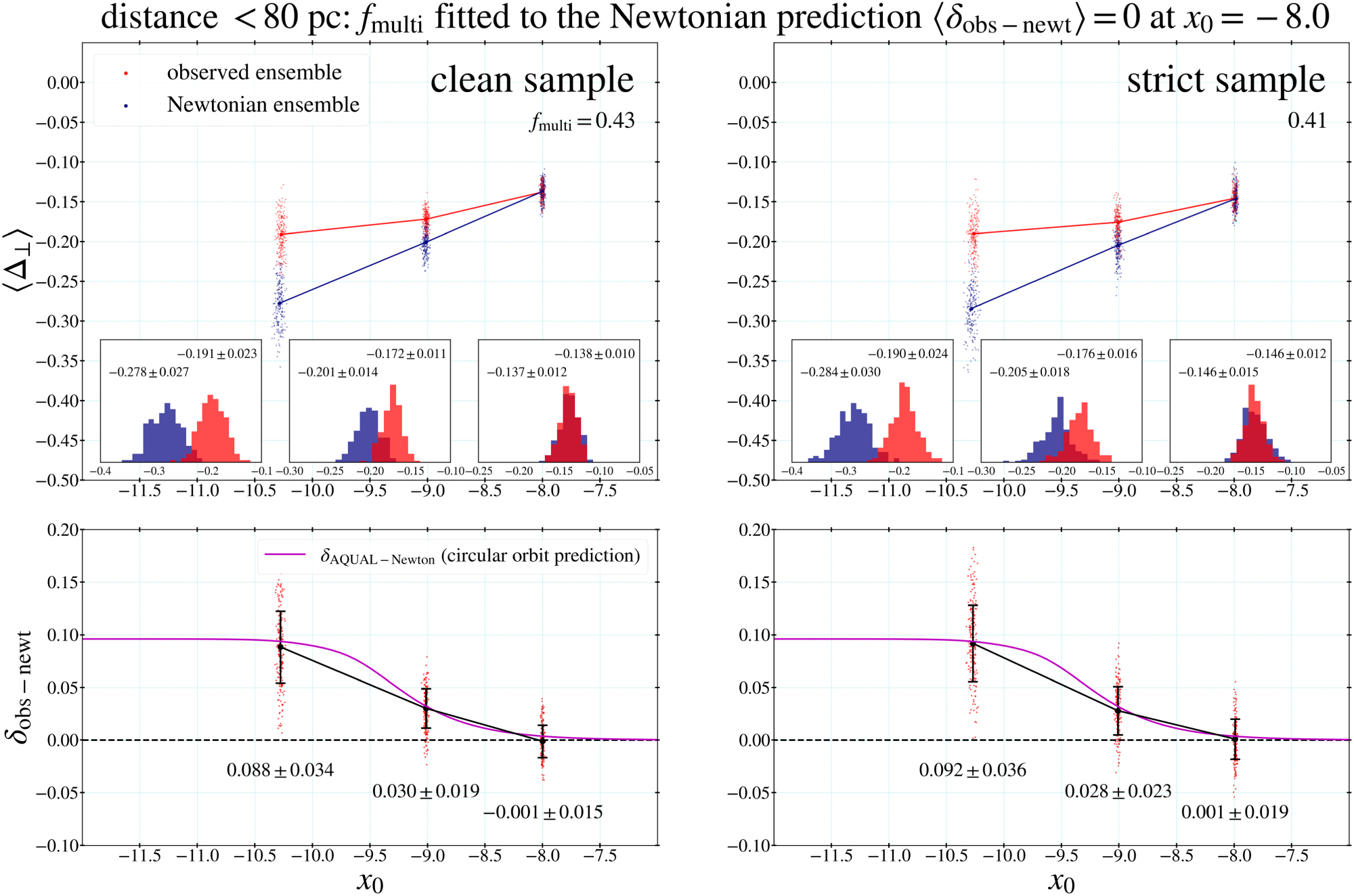