


Abstract
During the Zwicky Transient Facility (ZTF) Phase I operations, 78 hydrogen-poor superluminous supernovae (SLSNe-I) were discovered in less than 3 yr, constituting the largest sample from a single survey. This paper (Paper I) presents the data, including the optical/UV light curves and classification spectra, while Paper II in this series will focus on the detailed analysis of the light curves and modeling. Our photometry is primarily taken by ZTF in the g, r, and i bands, and with additional data from other ground-based facilities and Swift. The events of our sample cover a redshift range of z = 0.06 − 0.67, with a median and 1σ error (16% and 84% percentiles) of  . The peak luminosity covers −22.8 mag ≤ Mg,peak ≤ −19.8 mag, with a median value of
  mag. The light curves evolve slowly with a mean rest-frame rise time of trise = 41.9 ± 17.8 days. The luminosity and timescale distributions suggest that low-luminosity SLSNe-I with a peak luminosity ∼−20 mag or extremely fast-rising events (<10 days) exist, but are rare. We confirm previous findings that slowly rising SLSNe-I also tend to fade slowly. The rest-frame color and temperature evolution show large scatters, suggesting that the SLSN-I population may have diverse spectral energy distributions. The peak rest-frame color shows a moderate correlation with the peak absolute magnitude, i.e., brighter SLSNe-I tend to have bluer colors. With optical and UV photometry, we construct the bolometric luminosity and derive a bolometric correction relation that is generally applicable for converting g, r-band photometry to the bolometric luminosity for SLSNe-I.
Export citation and abstract BibTeX RIS
1. Introduction
Superluminous supernovae (SLSNe) constitute a rare class of stellar explosions that were first discovered over 15 years ago (i.e., SN 2005ap; Quimby et al. 2007). Their peak luminosities (1043−44 erg s−1) are 10–100 times higher than those of normal Type Ia and core-collapse supernovae (SNe). Their light curves (LCs) usually evolve rather slowly, with rise times of ∼20–100 days. The combination of these two features cannot be explained by conventional SN models, i.e., standard radioactive decay (Kasen 2017). With the discovery of the first few SLSNe (SN 2005ap, SN 2006gy, SN 2007bi, and SN 2008es), it was quickly recognized that, like normal SNe, SLSNe can be divided into two spectroscopic subclasses, one with hydrogen emission lines (SLSNe-II; Gezari et al. 2009; Miller et al. 2009; Inserra et al. 2018b) and the other without hydrogen (SLSNe-I; Ofek et al. 2007; Quimby et al. 2007; Smith et al. 2007; Gal-Yam et al. 2009; Gal-Yam 2012). In recent years, the subclass of H-poor but Helium-rich SLSNe (SLSNe-Ib) was first identified by Quimby et al. (2018), with a later sample from Yan et al. (2020).
Three popular models have been proposed to explain the extraordinary radiative power of SLSNe. One involves energy injection from a central engine, such as the spindown of a fast-rotating neutron star (magnetar; Kasen & Bildsten 2010; Woosley 2010). Alternatively, the interactions between the SN ejecta and dense circumstellar material (CSM) can efficiently convert kinetic energy into radiation (Chevalier & Irwin 2011; Chatzopoulos et al. 2013). Finally, some SLSNe could be powered by massive amounts of 56Ni synthesized in a pair-instability SN explosion of low-metallicity stars with masses >140 M⊙ (Woosley et al. 2007; Kasen et al. 2011). It is commonly accepted that most SLSNe-II are analogous to Type IIn SNe (Schlegel 1990; Filippenko 1997) and primarily powered by ejecta interactions with the dense CSM (Ofek et al. 2007; Miller et al. 2010; Chevalier & Irwin 2011), while a small fraction show broad Hα features with no signs of strong interaction in their spectra, e.g., SN 2008es, SN 2013hx, and PS15br (Gezari et al. 2009; Miller et al. 2009; Inserra et al. 2018b), although interactions are likely still required in these events (Kangas et al. 2022).
Between 2005 and 2009, a handful of SLSNe were discovered by several untargeted transient surveys that were not specifically targeting bright nearby galaxies. This small number of luminous events sparked a flurry of studies on both the theory and observation of SLSNe. The next big advance in this field came between 2009 and 2016, when large-area untargeted transient surveys started operating. For example, the Palomar Transient Factory (PTF; Law et al. 2009), the Pan-STARRS1 Medium Deep Survey (PS1 MDS; Chambers et al. 2016), the Catalina Real-time Transient Survey (Drake et al. 2009), the All-Sky Automated Survey for SuperNovae (ASAS-SN; Shappee 2014), the Dark Energy Survey (DES; The Dark Energy Survey Collaboration 2005), and the Gaia Photometric Science Alerts (Gaia; Hodgkin et al. 2021) made major contributions to the discoveries of several dozen SLSNe, at both low (z ∼ 0.2) and high redshift (z ∼ 1; Nicholl et al. 2015; De Cia et al. 2018; Lunnan et al. 2018; Quimby et al. 2018; Angus et al. 2019). However, with over ∼90 SLSNe-I having been discovered by the end of 2017, many questions regarding their physical nature still remain unclear. For example, the SLSN volumetric rates are poorly constrained, with only estimates from small SLSN-I samples (Quimby et al. 2013; McCrum et al. 2015; Prajs et al. 2017; Frohmaier et al. 2021). Attempts to examine the statistical distributions, such as luminosity functions, have also been quite limited, due to the small number statistics.
Assembling a large sample of low-z SLSNe with a well-defined survey volume and cadence is one of the goals of the Zwicky Transient Facility (ZTF; Bellm et al. 2019a; Graham et al. 2019; Masci et al. 2019). ZTF utilizes a 600 megapixel camera mounted on the Palomar Samuel Oschin 48 inch Schmidt telescope to reach a 47 deg2 field of view (Dekany et al. 2020). ZTF can cover the full northern sky in 3 days, down to a 5σ limiting magnitude of 20.5–20.8 mag, which is about 3.5 and 0.5 mag deeper than that of ASAS-SN (Shappee 2014) and the Asteroid Terrestrial-impact Last Alert System (ATLAS; Tonry et al. 2018), respectively. The ZTF survey offers several advantages for discovering rare transient events, such as SLSNe. It is an untargeted, all-sky, and moderately high-cadence survey, probing large volumes with its large area coverage and deep sensitivity limits. Its well-defined survey strategy—area coverage and cadence—also makes it possible to quantify the survey efficiency.
ZTF conducted several surveys with different cadences (ranging from minutes to days) and area coverages during its phase I operations (Bellm et al. 2019b). Among them, a particularly important one for extragalactic transient studies is the Northern Sky Public Survey. ZTF covered roughly the entire northern sky accessible from Palomar, corresponding to a total sky area of ∼23,675 deg2. Every 3 days, each field was observed once in the g band and once in the r band, with an interval of at least 30 minutes between the observations.
Between 2018 March 17 and 2020 October 31, ZTF Phase I 26 discovered and spectroscopically confirmed 85 SLSNe-I, 6 SLSNe-I.5 (classified as SLSNe-I, but showing H lines after the peak), and 61 SLSNe-II (defined as SNe II with peak magnitudes brighter than −20.0 mag). The numbers of SLSNe discovered by ZTF from 2018 to 2020 (about 60 per year) are roughly five to seven times higher than those detected in any previous years. The SLSN-I sample will be the focus of a series of three papers. Paper I (this paper) presents the observational data and analysis of the overall observational properties. Paper II (Chen et al. 2022) discusses the LC modeling and analysis of the LC morphology. Paper III (L. Yan et al. 2023, in preparation) will present the derived SLSN-I volumetric rates and luminosity functions at z ≤ 0.7. Several additional papers, based on some individual SLSNe discovered during the ZTF Phase I operations, have recently been published. Lunnan et al. (2020) showcased the first four SLSNe-I discovered by ZTF during its science commissioning phase. Yan et al. (2020) presented the discovery of six He-rich SLSNe-I (SLSNe-Ib), revealing additional constraints on the progenitor mass-loss history.
This paper is organized as follows. Section 2 introduces the selection and classification of this sample. Section 3 presents the photometry from ZTF and other facilities. Section 4 discusses our methodology, with various photometric corrections and the calculations of peak absolute magnitudes. The measurements of timescales, colors, blackbody temperatures, and bolometric luminosities are presented in Section 5. Section 6 summarizes the conclusions. Throughout the paper, all magnitudes are in the AB system, unless explicitly noted otherwise. We adopt a ΛCDM cosmology, with H0 = 70.0 km s−1 Mpc−1, ΩM = 0.3, and ΩΛ = 0.7.
2. The SLSN-I Sample from ZTF I
During the phase I survey, ZTF discovered 85 SLSNe-I. This paper focuses on 78 of these 85 events, whose LCs had turned over from their peaks by 2020 October 31, enabling better LC modeling. Of these 78 SLSNe-I, seven can be classified as He-rich SLSNe-Ib, including six published by Yan et al. (2020) and one by Terreran et al. (2020). For completeness, this sample paper also includes the four sources published in Lunnan et al. (2020). In addition, S. Schulze et al. (2023, in preparation) will focus on an extremely slow and peculiar SLSN-I, ZTF18acenqto (SN 2018ibb), having provided the derived parameters to include in our catalog.
Table A1 compiles the metadata for each of the targets, including the internal ZTF name, the IAU name, R.A. (R.A.), decl. (decl.), redshift, Galactic extinction E(B − V), discovery group, and additional information on spectral classification. Our sample covers the redshift z ∼ 0.06–0.67, with a median of  . All of the redshifts in our sample are determined using the narrow emission lines from the host galaxy, except for nine events without host lines. The redshifts for these nine events are estimated from template matching, by running superfit (Howell et al. 2006) over a range of z values. These redshifts are less accurate and marked with ⋆ in Table A1. There are two additional events, ZTF19abcvwrz (SN 2019aamx) and ZTF19aawsqsc (SN 2019hno), which also have less accurate redshifts because, of the low signal-to-noise ratios of the Mg ii
λλ 2796, 2803 absorption lines in their host galaxy spectra. Figure 1 displays the redshift distribution of the full sample, including those derived from template fitting. To avoid possible biases caused by the choice of histogram grids, we apply kernel density estimation on all the histograms in this paper, using a Gaussian kernel offered by the machine-learning package Scikit-learn (Pedregosa et al. 2011), as shown in Figure 1.
. All of the redshifts in our sample are determined using the narrow emission lines from the host galaxy, except for nine events without host lines. The redshifts for these nine events are estimated from template matching, by running superfit (Howell et al. 2006) over a range of z values. These redshifts are less accurate and marked with ⋆ in Table A1. There are two additional events, ZTF19abcvwrz (SN 2019aamx) and ZTF19aawsqsc (SN 2019hno), which also have less accurate redshifts because, of the low signal-to-noise ratios of the Mg ii
λλ 2796, 2803 absorption lines in their host galaxy spectra. Figure 1 displays the redshift distribution of the full sample, including those derived from template fitting. To avoid possible biases caused by the choice of histogram grids, we apply kernel density estimation on all the histograms in this paper, using a Gaussian kernel offered by the machine-learning package Scikit-learn (Pedregosa et al. 2011), as shown in Figure 1.

Figure 1. The distribution of the redshifts for the sample of 78 SLSNe-I presented in this paper. Other SLSN-I samples are plotted as hollow bars, for comparison. The dashed line and shaded area mark the median value and 1σ error (the 16% and 84% percentiles) of the ZTF sample,  . The black solid line shows the kernel density estimation of the distribution.
Download figure:
Standard image High-resolution imageSeveral SLSN-I samples from different surveys—including PS1, DES, and PTF, as well as samples collected from the literature by Nicholl et al. (2015) and Inserra et al. (2018a)—have revealed many important properties of SLSNe-I. Compared with these previous samples, our sample size is significantly larger, and the observing cadence is also better, as shown in Table 1. These two key features allow us to investigate the LC properties of SLSNe with much better statistics.
Table 1. SLSN Samples
| Source | Candidates | Redshift Range | Observing Cadence a | Reference |
|---|---|---|---|---|
| (Rest-frame Days) | ||||
| Literature | 25 b (14) | 0.10 – 1.19 | ⋯ | Nicholl et al. (2015), Inserra et al. (2018a) |
| PS1 | 17 | 0.32–1.57 | 2.30 | Lunnan et al. (2018) |
| DES | 22 | 0.22–2.00 | 3.65 | Angus et al. (2019) |
| PTF | 26 | 0.06–0.74 | 2.26 | De Cia et al. (2018) |
| ZTF | 78 | 0.06–0.67 | 1.45 | This paper |
Notes.
a The median value of the observing cadence in the rest frame. b Including 11 SLSNe-I from the PTF and PS1 samples and 14 independent SLSNe-I.Download table as: ASCIITypeset image
2.1. Photometric Selection
Here, we briefly describe the photometric selection system of our SLSN-I candidates. Daily ZTF alerts are ingested into a dynamic science portal called the GROWTH Marshal (Kasliwal et al. 2019). A filter is implemented within the Marshal to select SLSN candidates. The candidates passing the filter are not automatically saved; instead, each week, a human scanner has to visually examine the LC of each candidate selected by the filter and make a decision as to whether it is worth being saved. The subsequent spectral follow up is based on the human-saved candidates. This filter adopts several cutoff conditions, including: (1) it is not moving—the same alert is detected in two consecutive epochs with Δt > 0.02 day; (2) it is not a star, based on the Sloan Digital Sky Survey (SDSS) star–galaxy scores (Tachibana & Miller 2018); (3) the exclusion of bogus, alerts based on the scores constructed by Duev et al. (2019); (4) it is not in the galactic plane, with galactic latitude ∣b∣ > 7°; and (5) variability has not been detected at this location more than a year prior to the alert.
In addition, we assign numerical scores to several properties, including: (1) slowly rising events; (2) faint blue hosts; (3) the spatial location of the transient relative to the center of the host (against nuclear transients); (4) the brightness of the candidate relative to the host brightness (against faint transients); and (5) the time interval between the first detection and the last one (against very long-lived transients, like active galactic nuclei). This candidate filter gives high scores (thus preferences) to slowly rising events with faint blue hosts. For example, a candidate rising at least 20–25 days, with a faint host galaxy, will have a high score, pass the filter, and also be saved by the human scanner.
We note that the ZTF collaboration has multiple transient groups that also perform daily alert stream scanning, and most transient candidates can be saved by multiple groups—for example, the ZTF Bright Transient Survey (BTS; Fremling et al. 2020), the ZTF Census of the Local Universe (De et al. 2020), the fast transient group, the stripped envelope SN group, and the ZTF nuclear transient group. Therefore, the classification of a specific SLSN-I candidate can also be drawn from other classification efforts, most noticeably the BTS. A few classifications are taken from the Transient Name Server reported by external groups. But almost all of these externally classified sources were also identified as candidates by our filter. The filtering method will be described in detail in the forthcoming work.
With the above selection criteria, on the order of 50 candidates per week are saved, before going through another round of vetting when the spectral classification observations are planned. Any candidates brighter than 18.5 mag are classified by the ZTF BTS. The classification efficiency at ≤18.5 mag is very high, close to 95% (Fremling et al. 2020; Perley et al. 2020). We anticipate that our catalog is almost entirely complete for SLSNe within the ZTF footprint peaking at magnitudes brighter than 18.5 mag, and highly complete to 19.0 mag. For magnitudes fainter than 19.0 mag (44 of 78 events in total), there may be biases, primarily related to the nature of the host and/or the rising phase of the LC, which will be examined in future work. The detailed structure of the LC, e.g., the presence of bumps, was not a crucial factor for selection or triggering follow up.
Our efforts of spectroscopic classification were primarily focused on SLSN candidates fainter than 18.5 mag, using the Spectral Energy Distribution Machine (SEDM; Blagorodnova et al. 2018) and the Double Beam Spectrograph (DBSP; Oke & Gunn 1983) mounted on the Palomar 60 inch (P60) and 200 inch (P200) telescopes, respectively. Additional facilities include the Low Resolution Imaging Spectrometer (LRIS; Oke et al. 1995) on the Keck I telescope, the Alhambra Faint Object Spectrograph and Camera (ALFOSC) on the 2.56 m Nordic Optical Telescope (NOT), the SPectrograph for the Rapid Acquisition of Transients (SPRAT) on the 2 m Liverpool Telescope (LT), and the Intermediate-dispersion Spectrograph and Imaging System (ISIS) on the 4.2 m William Herschel Telescope (WHT). The basic information about the classification spectra is listed in Table A2. The spectral reduction is performed using various standard reduction pipelines. This includes the SEDM automated pipeline (Rigault et al. 2019), the pyraf-dbsp package (Bellm & Sesar 2016) and DBSP_DRP (Roberson et al. 2022) pipelines for the DBSP data, and the LPipe package (Perley et al. 2019) for the LRIS data.
Finally, we note that the SLSN project has at least 0.5–1 night of DBSP time on P200 per month for spectral classification (PI: Yan). More quantitative discussions on the completeness of the spectral classification will be included in Paper III.
2.2. Spectral Classification
Every event in our sample has at least one spectrum, and most have multi-epoch spectra. The hallmark spectral features for SLSNe-I are the five O ii absorption features in the wavelength range of 3737−4650 Å in prepeak and/or near-peak optical spectra. These were identified and discussed in Quimby et al. (2011, 2018). We utilize the large SLSN-I spectral template library assembled by Quimby et al. (2018), and update the library by adding the missing phase information to some of the templates. Our classification relies on matching with the spectral templates using SNID (Blondin & Tonry 2007) and superfit.
To determine the best-matched spectral templates, we run both superfit and SNID on the smoothed spectra, with host galaxy emission lines removed and redshifts fixed for most sources. If the spectrum of an SLSN-I has a good match with that of an SN Ic, but its g-band peak luminosity is higher than −20.0 mag, we classify this candidate as an SLSN-I, since many SLSNe-I develop spectra similar to those of SNe Ic after the peak (Pastorello et al. 2010; Quimby et al. 2018; Gal-Yam 2019).
In the Appendix, Figure A1 presents the best-fit spectral templates for each event in our sample, with the event name, phase, and template information labeled after the spectra. The phases are measured relative to the rest-frame g-band peak in this paper. We note that the phase differences between the observed spectra of our SLSNe-I and the templates in the library are not zero, but generally within 30 days (rest frame). This is not surprising, since SLSNe-I can have similar photospheric spectra, but different LC evolution timescales (see Kangas et al. 2017; Quimby et al. 2018).
The above classification procedure can sometimes give ambiguous results for a small number of events—i.e., two events for our sample. In these cases, we rely on additional LC information, such as the rise time and peak luminosity, to break the degeneracy. For example, ZTF19aacxrab (SN 2019J) and ZTF19aaqrime (SN 2019kwt) are almost equally well matched with the spectral templates of SN Ia and SLSN-I. In the case of SN 2019J, although the overall spectral features broadly match with those of SNe Ia, its spectrum lacks S ii λλ 5433, 5606 commonly seen in SNe Ia. In addition, because of their slow-rising LCs and high peak luminosities (i.e., SN 2019kwt has Mg ∼ −22.8 mag), we adopt the SLSN-I classifications corresponding to the template spectra of SN 2007bi and PTF09cnd, respectively.
In summary, the 78 sources listed in Table A1 can be classified as SLSNe-I according to the features of their spectra and LCs. The classification spectra are made available to the public as part of the electronic data at the Journal website, and they will be uploaded to the Weizmann Interactive Supernova Data Repository (Yaron & Gal-Yam 2012). 27
3. Observations and Data
3.1. ZTF Data and Forced Photometry
The bulk of the photometric data comes from ZTF, including the data from the public survey with a 3 day cadence and the ZTF partnership and Caltech surveys with a faster cadence (≤2 days) over smaller areas (Bellm et al. 2019b).
The IPAC ZTF pipeline produces reference-subtracted images using the ZOGY algorithm (Zackay et al. 2016) and aperture photometry for all transients detected at ≥5σ. However, there are two issues with the LCs produced by this pipeline. One is that the reference images built in 2018 may contain signals from transients that exploded during the same period, for which the photometric offset needs to be corrected. The second issue is that the upper limits prior to the first detection are from aperture photometry and based on the image noise measured over the entire quadrant. This can significantly underestimate the transient signals.
To fix these two issues, we perform forced point-spread function (PSF) photometry using the software provided by IPAC. 28 With a code from Yao et al. (2019), we refine the astrometric position of each event by using only the images around the peak phase. The very early- and late-time forced photometry without transient signals allows us to compute baseline offsets to the LCs. In addition, we reject bad-quality data if: (1) the image processing and instrumental calibration fail to meet predefined quality criteria; (2) the robust estimate of the 1σ value of the spatial noise per pixel in the image is over 25; and (3) the seeing is larger than 5'', similar to what was used in Yao et al. (2019). The photometry of the same transient observed with different CCD quadrants can have a systematic offset. This problem is fixed by our photometric reprocessing as well. For the final photometric collections, a detection is defined as 4σ (3σ for Swift data) above the background, and an upper limit is computed at 3σ.
The ZTF astrometric and photometric systems are calibrated using the Gaia Data Release 1 data and the PS1 catalogs, respectively (for details, see Masci et al. 2019). The output magnitudes are in the AB system. The airmass and color term corrections are included when the photometry is calibrated to the PS1 system. The color information for color corrections (g − r for the g, r bands and r − i for the i band) is obtained from the g, r, i photometry taken at the same epoch, or neighboring observations.
3.2. Supplemental Photometry
3.2.1. P60, LT, and P200 Photometry
When ZTF is not able to take observations due to scheduling conflicts, bad weather, or when the transient is fainter than the ZTF detection limits, additional data are taken with SEDM on the P60 (Blagorodnova et al. 2018), the Optical imager of the Infrared-Optical suite of instruments (IO:O) on the LT (Steele et al. 2004), or the Wafer-Scale camera for Prime (WASP) 29 on the P200. All of the P60, LT, and P200 photometric results are obtained via PSF fittings, which are calibrated with the PS1 and SDSS (for the u band and some of P60 data only) standard stars. For the P60 data, the systematic errors between the PS1 and SDSS systems may introduce an additional uncertainty of 0.01 mag in the r and i bands and a larger error (up to 0.25 mag) in the g band. The airmass and color term corrections are included in all the P60/LT/P200 data. The P60 data are processed using the software Fpipe (Fremling et al. 2016), and the image subtraction uses the SDSS references, while the LT photometric data are processed with the software specifically built for IO:O (Steele et al. 2004; Fremling et al. 2016, K. Taggart et al. 2023, in preparation). The IO:O collects data in the SDSS u, g, r, i, and z bands, and image subtraction is performed using reference images from PS1 or SDSS (for the u band only). The P200 data are processed using the software AutoPhOT (Brennan & Fraser 2022), and the PS1 reference images are used for image subtractions before performing photometry.
3.2.2. Swift Data
27 of 78 events in our sample have observations from the UV/Optical Telescope (UVOT; Roming et al. 2005) aboard the Neil Gehrels Swift Observatory (Gehrels et al. 2004). We retrieved the UVOT data from the NASA Swift Data Archive, 30 and used the standard UVOT data analysis software distributed with HEASoft version 6.19 31 (Nasa High Energy Astrophysics Science Archive Research Center 2014), along with the standard calibration data. We manually define sky background apertures devoid of any sources. Four events in our sample—namely, ZTF18aavrmcg (SN 2018bgv), ZTF18acslpji (SN 2018hti), ZTF19aawfbtg (SN 2019hge), and ZTF19abpbopt (SN 2019neq)—have bright host galaxies. We therefore requested host galaxy images at very late phases, when the SNe had faded. The photometry for these four objects was obtained by subtracting out the host galaxy fluxes. For most of the other events, their host galaxies are very faint and contribute no more than 10% of the SN fluxes in the UV bands, so no host galaxy subtractions are applied.
All the photometry data are listed in Table A3 and are available to the public in electronic format at the Journal website.
4. The Observed LCs
The observed LCs for the full sample are presented in Figures A2–A7, where the left Y-axis is the apparent magnitude and the X-axis is the rest-frame days relative to the g-band peak phase. For a small number of events without a g-band peak phase, we use the r-band peak phase as the reference. Table A3 contains the complete upper limits over much wider time ranges (early and late times) than those shown in the plots. For a better display, we plot only a small number of the photometric upper limits.
One striking feature apparent in Figures A2–A7 is that a large fraction of the LCs in our sample show significant undulations, and some have multiple peaks. In Paper II, we find that 18%–44% of the well-sampled SLSNe-I have LC undulations. Among a small subset of SLSNe-I with early phase coverage, 6%–44% show early double-peak LCs. Quantitative analysis of the LCs and discussions of these features are included in Paper II.
4.1. Magnitude Corrections
4.1.1. Extinction Corrections
The galactic reddening E(B − V) is taken from the Schlafly & Finkbeiner (2011) dust map, using the NASA/IPAC InfraRed Science Archive database. The extinction corrections at different wavelengths are computed using the empirical dust extinction laws of Fitzpatrick & Massa (2007), with RV = 3.1.
Previous studies have shown that SLSN-I hosts are mostly low-mass metal-poor dwarf galaxies (Lunnan et al. 2014, 2015; Leloudas et al. 2015; Angus et al. 2016; Perley et al. 2016; Chen et al. 2017a; Schulze et al. 2018). This is the case for most of the events in our sample. Because their LCs do not show particularly red colors at prepeak phases, we do not make any host galaxy reddening corrections to these events. However, a small fraction of the SLSN-I hosts are massive (109−10 M⊙; Perley et al. 2016; Chen et al. 2017b), and the host galaxy reddening in such cases can be large. We find that seven events in our sample (Table 2) have non-negligible host galaxy reddening. They either reside in bright hosts (Mr ≲ −18.5 mag) or have redder (g − r) colors at peak than average (see Figure 8), which are presumably due to host galaxy reddening.
Table 2. Host Galaxy Reddening
| Name |
 (mag) (mag) | Method |
|---|---|---|
| SN 2018don | 0.4 a | spec.temp |
| SN 2018kyt | 0.11 | line ratio |
| SN 2019kwt | 0.22 | line ratio |
| SN 2019aamx | 0.07 | spec.temp |
| SN 2019aamu | 0.23 | spec.temp |
| SN 2019stc | 0.18 | line ratio |
| SN 2020xkv | 0.24 | spec.temp |
Note.
a Estimated in Lunnan et al. (2020).Download table as: ASCIITypeset image
The host galaxy reddening is difficult to measure accurately, but it can be roughly estimated using two different methods. The first one uses the Balmer line ratio measured from the host galaxy spectra. Without dust attenuation, the predicted line ratio between Hα and Hβ remains constant over a wide range of temperatures and electron densities in the nebular regions (e.g., Hα/Hβ ≈ 2.86; Osterbrock & Ferland 2006). The attenuation caused by dust scattering is wavelength-dependent and stronger at shorter wavelengths. This method is affected by both stellar and SN absorption features. We remove the stellar Balmer absorption using FIREFLY (Wilkinson et al. 2017), before we measure the line flux, but we ignore the influence of SN features. This method is applied to the host spectra of ZTF18acyxnyw (SN 2018kyt) and ZTF19acbonaa (SN 2019stc). Note that the SN location may not coincide with the H ii region responsible for the Balmer lines, so the real extinction at the SN site could be different from the inferred value. But such an estimation is at least an indicator of whether the galaxy has significant dust.
The second method is to infer the host galaxy reddening by matching the observed spectrum (including the spectral continuum slope and absorption features) with an SLSN-I template with negligible extinction and at a similar phase. For this method, the assumption is that the observed red spectral color is due to the host galaxy reddening. The results from this method are very uncertain, but offer crude extinction estimates for those events without host emission lines. This method is applied to ZTF18aajqcue (SN 2018don), SN 2019aamx, and ZTF19acvxquk (SN 2019aamu), whose spectra lack distinct Balmer emission lines from host galaxies. For example, to match the near-peak spectrum of SN 2018don, the t ∼ + 54 day template spectrum of SN 2007bi is required to be reddened by E(B − V) ∼ 0.4 mag (Lunnan et al. 2020). Similarly, the +9 day spectrum of SN 2019aamu matches well with the −7 day template spectrum of PTF12gty, after considering a host galaxy reddening of E(B − V) = 0.23 mag. And the +13 day spectrum of SN 2019aamx matches well with the +22 day template spectrum of PTF09cwl with E(B − V) =0.07 mag (shown in Figure A1). Note that both PTF12gty and PTF09cwl have a faint dwarf host, so their host galaxy reddenings are assumed to be negligible (Perley et al. 2016; Quimby et al. 2018).
For SN 2019kwt and ZTF20abzaacf (SN 2020xkv), we applied both of the above methods, since their spectra contain strong SN signals and we are not able to remove the stellar absorption or SN features. The derived E(B − V) for SN 2019kwt is 0.22 mag from the host galaxy spectrum and 0.18 mag from template matching, which appear to be consistent. In the case of SN 2020xkv, the E(B − V) derived from the spectral matching ranges from 0.22–0.26 mag, in contrast to the lower value (0.17 mag) inferred from the Balmer decrement. Its spectrum has a very low signal-to-noise ratio at Hβ, and with both being highly uncertain measurements, we adopt the average value of 0.24 mag from the template matching method.
4.1.2. The K-corrections
The absolute g-band peak magnitude is one of the key parameters of SLSNe-I. Proper estimates of this value require proper K-corrections to derive reliable rest-frame values, either in the g band for sources at z ≤ 0.17 or in the r band for sources at z > 0.17. This switch is chosen because the observed r band LC at z > 0.17 is closer to the rest-frame g band in wavelength.
Most events in our sample have at least one spectrum around the LC peak (i.e., ≲20 days in the rest frame), which allow us to compute the K-corrections using the formula described in Hogg et al. (2002). For those without spectra near the peak phases, we apply a constant K-correction of  . This approximation is not too far from the spectral estimates, as shown below.
Figure 2 compares the calculated K-corrections based on the observed spectra (blue dots) and an assumed 104 K blackbody spectral energy distribution (SED; green line) with the constant correction (black line). The constant value of  appears to capture most of the corrections within a range of ±0.1 mag (the shaded region) for SLSNe-I at 0.06 < z < 0.67. We list the K-corrections for each event in Table A4.

Figure 2. K-corrections from the observed band to the rest-frame g band for SLSNe-I around the peak. The blue points represent the corrections computed from the observed spectra. The black line shows the constant correction of  , with an uncertainty of 0.1 mag shown by the gray shaded area. The green line shows the correction calculated by assuming a blackbody spectrum with a temperature of 104 K. The break at z = 0.17 is caused by the change of the observed band (from the g to the r band).
Download figure:
Standard image High-resolution image4.1.3. The S-corrections
As the g-, r-, and i-band photometry of the SLSNe-I presented in this work is obtained from four different telescopes, the errors caused by filter differences need to be evaluated. Since most of the data are from the ZTF itself, we choose to correct the LT/P200/P60 photometry to that of the ZTF filters. Following the method of Stritzinger et al. (2002, 2005), Pignata et al. (2008), and Wang et al. (2009), the correction between the different instruments (known as the S-correction) can be computed using

where Mλ1 is the SN synthetic magnitude computed with the response functions of the ZTF λ1 filter and mλ1 and mλ2 are the SN synthetic magnitudes computed with the LT/P200/P60 filters. CTλ1 is the color term and ZPλ1 is a zeropoint, which are measured by convolving the ZTF filters with a large sample of spectrophotometric Landolt standard stars from Stritzinger et al. (2005). The response function above includes filter transmission, detector quantum efficiency, and atmospheric transmission.
As S-corrections are spectrum-dependent, and accurate measurements at any given epoch require far more SLSN-I spectra than we have in this work, we use the S-correction values computed from the spectra as an additional 1σ error in photometry, and add them to the existing errors of LT/P200/P60 photometry in quadrature. The additional 1σ errors due to the S-corrections are listed in Table 3.
Table 3. The Estimated Error Caused by the S-correction
| Telescope | Filter | ||
|---|---|---|---|
| g(mag) | r(mag) | i(mag) | |
| LT | 0.018 | 0.044 | 0.030 |
| P60 | 0.042 | 0.030 | 0.026 |
| P200 | 0.023 | 0.030 | 0.025 |
Download table as: ASCIITypeset image
4.2. Empirical LC Fitting Method
The LC analysis requires estimates of various parameters—such as the peak magnitude, rise time, and rise rate—which all involve numerical interpolation and fitting. We adopt a machine-learning algorithm, Gaussian Process (GP) regression, which has various kernel functions. The GP interpolation can reduce the influence of outliers and gives robust error estimates. We use a composite kernel, which is the sum of a Matérn kernel with a white noise kernel. We tested Matérn kernels with ν parameters of 3/2 (Matérn 3/2; Inserra et al. 2018a; Angus et al. 2019; Lunnan et al. 2020) as well as ν = 5/2 (Matérn 5/2). When we compute the peak magnitudes and phases, a GP fit with Matérn 3/2 is performed in the flux space. The Python package george (Ambikasaran et al. 2016) and Scikit-learn give comparable results.
4.3. LCs in Absolute g-band Magnitudes
To set an approximate luminosity scale, we also plot the absolute magnitude on the right Y-axis of Figures A2–A7. This is calculated by assuming a constant K-correction of  . In these figures, the LCs have been corrected for galactic and host galaxy reddening, whenever possible.
To calculate the apparent peak magnitude and phase, we run the GP to interpolate the LCs in flux space. The errors are shown as 1σ uncertainties. The g-band absolute peak magnitudes are derived using Mg
= mg
− μ − KC, where μ is the distance modulus, KC is the K-correction, and mg
is the apparent g-band magnitudes, corrected for both the host (in the rest frame) and galactic extinction (in the observed frame). The rest-frame g-band absolute peak magnitudes and the peak dates are tabulated in Table A4. The peaks of some events are not well constrained, due to the poor sampling around the peak. Figure 3 shows the distribution of the g-band absolute peak magnitudes (Mg
) for the ZTF sample, ranging from −19.8 mag to −22.8 mag, with a median and 1σ error of  mag. Both our median value and dispersion are consistent with those of previous samples.

Figure 3. The distribution of the rest-frame g-band absolute peak magnitudes. The dashed line and shaded region mark the median value and 1σ dispersion,  mag. The black solid line shows the kernel density estimation of the distribution. Other SLSN-I samples are plotted in different hatching patterns for comparison. The DES and PS1 samples are measured at 400 nm, which is bluer than the g band (472 nm).
Download figure:
Standard image High-resolution imageThe weak bimodal distribution in the peak absolute magnitudes should not be overinterpreted, because this is the raw distribution function, without applying corrections for various selection biases (e.g., the Malmquist bias or the preference of our selection system for slowly rising events). Selection biases could also have a strong impact on the distribution of the timescales (e.g., Figure 5), the peak bolometric luminosities (e.g., Figure 16), and other photometric properties. The correct interpretation of these distributions requires a well-defined selection function for our sample—a detailed simulation of this, however, is well beyond the scope of this paper. Further studies (e.g., Paper III) are required to confirm these distributions.
5. LC Parameters
5.1. Rise/Decay Timescales–Fast and Slow SLSN-I Events
Traditional rise times, defined as the interval between the explosion date and the peak, are notoriously difficult to measure, especially for distant transients such as SLSNe-I. Although the ZTF detection can go down to 20.5–21.0 mag, at the median redshift of our sample it only probes an absolute magnitude of ∼−20 mag. The upper limits before the first detection cannot usually place strong constraints on the LC evolution in the very early phases, and only about one-third of our sample has high-quality early-time data. In addition, Anderson et al. (2018) show that an SLSN-I (SN 2018bsz) can have a long slowly rising "plateau," before a steeper, faster rise to the peak, which makes it harder to speculate on explosion dates without enough deep early data.
Instead of using the traditional rise time, we define trise/decay,x as the time interval between the peak and the flux when it is at a fraction x of the peak value. Here, the x factor can be 10% (Δmag = 2.5), or 1/e (Δmag ≈ 1.09). Time dilation is corrected for all timescale measurements. The derived trise,10% and trise/decay,1/e are listed in Table A4. The poorly constrained timescales are not included in the following analysis.
Figure 4 shows the direct proportionality between trise,1/e and trise,10% in the rest-frame g band. A linear fit gives trise,1/e = 0.80 trise,10% − 1.73 days with the 1σ uncertainty as small as ∼2.84 days. The small scatter implies that the LC rise rates in the very early phases do not have significant differences in our sample. The rise times trise,10% cover a wide distribution, ranging from 10 to 90 days, with the mean (median) value and a standard deviation of  days.
days.

Figure 4. The rise time measured at 10% of the peak flux trise,10% vs. that measured at 1/e of the peak flux trise,1/e. The vertical solid gray line marks the mean value of trise,10%, while the dashed and dotted lines represent the 1σ and 2σ uncertainties, respectively. The black solid line and shaded area show the linear fit to the measured timescales (trise,1/e = 0.80 trise,10% − 1.73 days) and the 1σ dispersion. The events with extreme timescales are highlighted in different colors.
Download figure:
Standard image High-resolution imageOf the total 56 SLSNe-I with trise,10% measurements, the two slowest rising events—SN 2018ibb and ZTF20aapaecd (SN 2020fyq)—stand out in Figure 4, with timescales longer than  days.
days.
For another slowly evolving event, ZTF20aadzbcf (SN 2020fvm), its trise,1/e reaches 91 days, which is suggestive of an unusually long rise time, although the trise,10% is not well constrained. SN 2020fvm has two LC peaks and we set the second—and also brighter—one as its main peak. If the first one is set as the main peak, its trise,1/e is around 48 days. The fastest event in our sample is SN 2018bgv (Lunnan et al. 2020), which rises to the peak in less than 10 days. Such a fast and luminous event is very rare, and it may be associated with the Fast Blue Optical Transients (Drout et al. 2014; Ho et al. 2021). Compared with previous SLSN-I samples, our sample contains slightly more fast-evolving events. For instance, nine of 56 events (9%–26%, calculated at a confidence level of 95%, based on Gehrels 1986) are found to have trise,1/e ≲ 15 days, while only five of 55 events (4%–18%) were reported in the previous samples.
Outside the ±1σ range, we have 10 fast-evolving events with  days and 10 slow events with
  days. The trise,10% shows a continuous distribution, and it cannot be divided into two separate fast and slow subclasses, as indicated by previous studies (Nicholl et al. 2015; De Cia et al. 2018).
Figure 5 shows a comparison of the rise and decay timescales measured at 1/e of the peak flux for 48 events. Both the rise/decay timescales show a distribution centered at ∼25–30 days, with an extended tail. For the whole sample, the rise and decay timescales show a strong positive correlation, with a Spearman correlation coefficient of ρ = 0.73 and a null probability p < 10−8; i.e., slowly rising events tend to decay slowly. Applying a linear fit, we find tdecay,1/e = (1.47 ± 0.07) trise,1/e + (0.35 ± 2.50) days, which is similar to what was found in previous studies (Nicholl et al. 2015; De Cia et al.2018).

Figure 5. Timescales measured at 1/e of the peak flux for the rising and declining portions of LCs. Normal SLSNe-I are shown with blue circles, while He-rich SLSNe-Ib are highlighted in red. The black dashed line and the shaded area show the best linear fit and 1σ error, tdecay = 1.47 trise + 0.35 days. The histograms along the horizontal and vertical axes show the distributions of the rise and decay timescales, respectively. The black solid lines show the kernel density estimation of the distributions. The timescales from other SLSN-I samples are plotted using smaller gray points, for comparison. The data from PTF are measured at 1 mag below the peak magnitude and are slightly shorter than the 1/e maximum (1.09 mag) timescales. And the data from the literature (Nicholl et al. 2015) and PS1 are measured from bolometric LCs and may have biases due to redshift and the SED.
Download figure:
Standard image High-resolution imageIt is interesting to note that four of the five SLSNe-Ib in the Yan et al. (2020) sample—namely SN 2018kyt, SN 2019hge, ZTF19acgjpgh (SN 2019unb), and ZTF20ablkuio (SN 2020qef)—have rise timescales that are 9–32 days longer than that of the rise–decay time correlation. The last SLSN-Ib, ZTF19aamhhiz (SN 2019kws), in the Yan et al. (2020) sample has a short rise time, but a much longer decay time. As noted in Yan et al. (2020), these SLSNe-Ib may have He-rich CSM, and CSM interaction may affect the LC evolution before or after the peak. Detailed modeling and discussions of the LCs are given in Paper II.
Although SNe Ic and SLSNe-I have similar postpeak spectra, they have very different peak luminosities and timescales. Figure 6 compares the peak Mg and rise times between normal SNe Ic, broad-lined SNe Ic (SNe Ic-BL), and SLSNe-I. The SLSNe-I are from our sample, while the normal SN Ic sample and the SN Ic-BL sample are taken from Barbarino et al. (2021) and Taddia et al. (2019), respectively. We exclude two bright SNe Ic from the literature, iPTF12gty and iPTF15eov, which can be better classified as SLSNe-I, as suggested by their authors. Both SN Ic samples are obtained from the (intermediate) PTF, which has a similar observation depth to ZTF. The overall distribution in Figure 6 is similar to that shown in De Cia et al. (2018). It should be noted that corrections for observational selection biases and volumetric corrections are required to interpret the distribution correctly. The peak Mg of the SLSNe-I is about 4 and 3 magnitudes brighter than those of the normal SNe Ic and SNe Ic-BL, respectively. All SLSNe-Ib have low luminosities and moderate rise times compared with normal SLSNe-I. SLSNe-I have significantly longer rise times and wider dispersions compared to those of SNe Ic. First, this is physically related to the fact that they have larger ejecta masses and more massive progenitor stars (see Paper II). Second, SNe Ic are primarily powered by radioactive decay, which has a constant timescale of energy injection. In the magnetar model proposed for SLSNe-I, the timescale of energy injection depends on the magnetic field B (∝B−2) and spin period P (∝P2). The LC width expands with the decrease of B (see Figure 2 of Kasen & Bildsten 2010). The large spread of their rise times could suggest that the magnetic field strengths of the neutron stars can vary over a wide range as well.

Figure 6. Rise times trise,10% vs. g-band absolute peak magnitudes Mg for SLSNe-I (this paper), normal SNe Ic (from Barbarino et al. 2021), and SNe Ic-BL (from Taddia et al. 2019). The Mg of the SN Ic and SN Ic-BL samples is computed from the r-band magnitudes using a color correction of ∼0.36 mag (Taddia et al. 2015; Prentice et al. 2016). The rise times of the SNe Ic and SNe Ic-BL are measured from the explosion dates in the r band, which are slightly longer than trise,10%. The SLSNe-Ib in our sample are highlighted.
Download figure:
Standard image High-resolution image5.2. Color and Blackbody Temperature
Understanding the variation and uniformity of the SLSN-I SEDs as a function of time should shed light on the physical nature of this population of stellar explosions. Although the complete characterization of the SLSN-I SEDs is beyond the scope of this paper, we can infer some basic properties by examining the distributions of the (g − r) colors and blackbody temperatures, since both parameters are determined by the transient SEDs.
Figure 7 shows the observed color evolution as a function of time. All the colors have been corrected for reddening, but not for K-corrections, since that requires better spectral coverage than we have. The overall (g − r) color trend evolves from blue (i.e., ∼−0.3 mag, hotter temperatures) at early phases to red, and reaches (g − r) ∼ + 0.8 mag at about two months after the peak. In our sample, four events have a peculiar color (temperature) evolution, and do not follow the general trend. We discuss these outliers below. We further examine the distribution of the observed (g − r) color obtained at the maximum light in Figure 8. At the peak phases, the median observed color is close to zero,  mag.
mag.

Figure 7. The observed (g − r) color evolution tracks with time. We highlight four events whose (g − r) color tracks do not follow the general trend in gray.
Download figure:
Standard image High-resolution image
Figure 8. The distribution of the (g − r) colors at the peak. Top panel: the red dotted line represents the original colors of the events with host galaxy reddening and the red area shows their corrected observed color. The blue area represents the observed colors of the events with only galactic extinction correction. After correction for host galaxy reddening, the observed (g − r) color at the peak has a median value with a 1σ dispersion of  mag, marked by the blue dashed line. The solid blue line shows the kernel density estimation of the distribution. Bottom panel: the green area represents the rest-frame colors of the events with K-correction. The rest-frame (g − r) color at the peak has a median value with a 1σ dispersion of
  mag, which is represented by the green dashed line. The solid green and blue lines show the kernel density estimations of the rest-frame colors and the observed colors (normalized to the number of rest-frame colors), respectively.
Download figure:
Standard image High-resolution imageFigures 7 and 8 show large scatters. The observed colors are not easy to interpret, because they sample different parts of the SEDs, depending on the transient redshifts. The proper measurements are the rest-frame color tracks, but reliable results would require many more spectra than our sample has. Here, we compute only the rest-frame (g − r) colors at the peak phase, using the color corrections computed from the near-peak spectra. The rest-frame (g − r) colors are corrected from the observed (g − r) for the events at z ≤ 0.17 and (i − r) for z > 0.17, if photometry data and spectra are available. All the peak colors are listed in Table A5. The green histogram in Figure 8 shows that the median rest-frame (g − r)rest,med is  mag, which is consistent with the −0.27 mag calculated from the PTF SLSN-I sample (De Cia et al. 2018). The large scatter in the peak rest-frame (g − r) indicates that the SEDs of SLSNe-I may show a diverse shape, and hence a wide range of blackbody temperatures.
Figure 9 illustrates a moderate correlation (ρ = 0.52, p < 10−3) between the peak rest-frame (g − r) colors and the g-band absolute peak magnitudes Mg,peak; i.e., brighter SLSNe-I tend to have bluer color, which was also previously found by Inserra & Smartt (2014) and De Cia et al. (2018) in smaller samples. If combined with the PTF sample from De Cia et al. (2018), the correlation becomes stronger (ρ = 0.56, p ≈ 2 × 10⁻⁵), and can be described by a linear function, Mg,peak = (11.5 ± 2.6) × (g − r) − (18.9 ± 0.5) mag, with a 1σ error of 1.7 mag. This correlation can be used in cosmological searches of SLSNe; e.g., Inserra et al. (2021). However, this is beyond the scope of this paper.

Figure 9. The correlation between the g-band absolute peak magnitudes Mg,peak and the rest-frame (g − r) colors. The linear fit and 1σ error are shown by the black line and the shaded area. The SLSN-I sample from this paper is marked in blue, while that from PTF (De Cia et al. 2018) is marked in orange.
Download figure:
Standard image High-resolution imageTo fit the blackbody temperature, we adopt a modified blackbody function, defined by ![${f}_{\lambda }=\max [\,0,\,1-A\,\times (1.0-\lambda /3000.0)]\times {B}_{\lambda }$](https://content.cld.iop.org/journals/0004-637X/943/1/41/revision1/apjaca161ieqn20.gif) , with Bλ
being the Planck function and A being the scaling factor. The modified blackbody function aims to quantitatively capture the variations in the UV spectral suppression for different events, as shown by the Hubble Space Telescope UV spectra of SLSNe-I (Yan et al. 2017, 2018). The scaling factor A is derived from the fitting at λ ≤ 3000 Å , set to zero at λ ≥ 3000 Å and fit in a range of 0–3. Larger scaling factors represent stronger suppression in UV, and A = 1 represents the SED function used in Nicholl et al. (2017). The error associated with the temperature is estimated using the Markov Chain Monte Carlo (MCMC) method.
, with Bλ
being the Planck function and A being the scaling factor. The modified blackbody function aims to quantitatively capture the variations in the UV spectral suppression for different events, as shown by the Hubble Space Telescope UV spectra of SLSNe-I (Yan et al. 2017, 2018). The scaling factor A is derived from the fitting at λ ≤ 3000 Å , set to zero at λ ≥ 3000 Å and fit in a range of 0–3. Larger scaling factors represent stronger suppression in UV, and A = 1 represents the SED function used in Nicholl et al. (2017). The error associated with the temperature is estimated using the Markov Chain Monte Carlo (MCMC) method.
Of the 78 events in our sample, only 15 have at least three epochs of Swift UV photometry for properly computing the blackbody temperatures. In Figure 10, the left panel shows the temperature evolution tracks for 12 events, and the right panel shows the other three with peculiar color/temperature evolutions. Although the statistics is not large, Figure 10 indicates the large temperature spread at any given phase, especially at the prepeak and peak phases. In the left panel, some SLSNe-I have high temperatures at ∼15,000 K at t ∼ −10 days, and cool down to ∼9000 K at +20 days. Interestingly, there are also two cooler SLSNe-I (i.e., SN 2019hge and SN 2019unb), with peak temperatures less than ∼10,000 K. Consistently, neither of them show clear O ii absorption lines in their classification spectra, which require a high ionization temperature (i.e., T ∼ 15,000 K; Quimby et al.2018). We perform a polynomial fit to the temperature tracks and derive T = 0.090201 t3 − 3.4306 t2 − 180.30 t + 13395 K and T = − 0.052720 t3 + 0.3319 t2 − 15.84 t + 9007 K for the high- and low-temperature tracks, respectively. These are shown as the blue and red shaded regions with the ±1σ uncertainty in Figure 10. Consistent with the temperature evolution, the (g − r) colors of low-temperature events are ∼0.2–0.3 mag redder than those of high-temperature ones at the peak, but become indistinguishable from those of the full sample +15 days after the peak.

Figure 10. Blackbody temperature evolution as a function of time. For comparison, we plot the temperature measurements from the PS1 sample in light gray. Left panel: we include 12 of 15 events with at least three epochs of UV data. We apply third-order polynomial fits to the temperature evolutions of two low-temperature events, SN 2019hge and SN 2019unb, and show the result with the 1σ error in the red shaded area. Similarly, the fit of 10 high-temperature events is shown by the blue shaded area. Right panel: we highlight the three extraordinary events and plot the 12 normal events in dark gray for comparison.
Download figure:
Standard image High-resolution imageMoreover, the color distribution plots suggest that there are more low-temperature SLSNe-I. For instance, 10 of 35 (29%) events are found to have redder peak rest-frame colors than the two low-temperature events (∼0.10 mag). However, these 10 events have no UV photometry available, thus no temperature measurements. It is possible that these 10 red events could also have low peak temperatures.
Combining the temperature measurements from the PS1 sample, we do see more low-temperature events. To better quantify the temperature distribution of SLSNe-I, we choose three typical epochs (i.e., t ∼ −10 days, 0 days, and +20 days relative to the rest-frame g-band peak) when sufficient data are available from the ZTF and PS1 sample. We show the temperature distribution at these epochs in Figure 11. At t ∼ −10 days, the temperature of SLSNe-I ranges from 7000 to 23,000 K for different events, while this range is 6000–20,000 K around the peak and 6000–12,000 K (excluding one special event, SN 2019szu) at t ∼ +20 days. As SLSNe-I evolve, both the median value and the spread of the temperature become smaller. This conclusion will still hold true if we expand the temporal range from −20 to +40 days, according to the temperature trend shown in Figure 10. Furthermore, the temperatures at any of the epochs in Figure 11 are found to show flat and unimodal distributions, indicating that SLSNe-I may have a continuous temperature distribution.

Figure 11. The temperature distributions (including both the ZTF and PS1 samples) at −10 days, 0 days, and +20 days relative to the rest-frame g-band peak. The dashed lines mark the median temperatures at different epochs; i.e., T ∼ 12,600 K at −10 days, T ∼ 12,000 K at the peak, and T ∼ 9200 K at +20 days. The solid lines show the kernel density estimation of the distribution.
Download figure:
Standard image High-resolution imageWe also measure the blackbody radius of the photosphere. As shown in the top panel of Figure 12, most events show a linearly expanding photosphere from explosion to 10−20 days around the peak. This is due to the recession of the photosphere being negligible during this phase. We apply a linear fit to measure the photosphere velocity, Vphot. In Paper II, we measured the velocities from the Fe ii and O ii absorption lines in the spectra. The velocity implied from the species Vion is expected to be higher than that from Vphot, since only the line features formed at higher velocity and lying outside the photosphere can be observed. As shown in the bottom panel of Figure 12, the distribution of ΔV = Vphot − Vion proves that most events have a negative ΔV and their Vphot is on average lower than Vion by about 2000–3000 km s−1. Two outliers, SN 2018bgv and SN 2018kyt, are found to have significantly higher Vphot than Vion. SN 2018bgv is the fastest-evolving event in our sample, while SN 2018kyt also exhibits relatively fast-evolving behaviors. Thus, the inconsistency between Vphot and Vion may be due to Vphot being the average velocity measured over a period of 10−20 days, while Vion is fast-evolving and measured at a single epoch. All of the measured temperature and radius values are listed in Table A6.

Figure 12. Top panel: the photosphere radius evolution as a function of time. Our measurements are plotted as open points, while those for the PS1 sample (Lunnan et al. 2018) are shown in gray lines, for comparison. For the events showing a linearly expanding photosphere before or at the peak, we apply a linear fit for them and plot the results with solid lines. Bottom panel: the distribution of the velocity difference between those derived from the photosphere radius (Vphot) and those measured from the absorption lines in the spectra (Vion). The blue and orange bars represent the values measured from Fe ii and O ii, respectively. The solid lines show the kernel density estimation of the distributions.
Download figure:
Standard image High-resolution imageIn summary, our measurements show that the SLSN-I have a wide range of temperatures, especially at early phases. While most SLSNe-I from ZTF have temperatures over 11,000 K at the peak, and cool down rapidly, there are also many lower-temperature and slowly evolving events. This indicates that the SEDs of SLSNe-I may have diverse shapes and different evolutionary tracks.
Finally, we discuss four peculiar events that have extraordinary color and temperature evolution, as shown in Figures 7 and 10.
SN 2018hti is well sampled in UV and shows notably higher temperatures and much bluer (g − r) colors compared with other events. Its LC can be well reproduced by a magnetar model (Lin et al. 2020). This event may represent some of the population with higher temperatures and bluer SEDs. However, we caution that this event has a very high galactic extinction E(B − V) = 0.4 mag. The dust extinction corrections in the UV bands are highly uncertain.
SN 2020fvm has two almost equally bright LC peaks (at phase ∼−60 and 0 days, respectively) and the longest 1/e maxima rise timescale, of 91 days. Both its color and temperature evolutions are peculiar. The (g − r) color around the two peaks shows a similar evolutionary trend, i.e., initially evolving from red to blue before the peak, and then turning red after the peak. During the phase from −75 days to +35 days, its temperature remains almost constant, at ∼10,000 K, which could be due to the absence of sampling. Such a long timescale and double-peak evolution are unexpected for a simple radiative cooling or magnetar model. Dessart (2019) examined the color evolutions for various configurations of magnetar models, and found that almost all have fairly blue colors in the early phase, with none showing a color change of ∼0.7 mag from red to blue. The ejecta interactions with an extended H-poor CSM could be a possible explanation.
ZTF19aanesgt (SN 2019cdt) has much redder color at +20 days after the peak, and it evolves much faster in comparison to the other objects in our sample. No temperature evolution is computed, due to the lack of UV data. This event is somewhat similar to SN 2018bgv, with both belonging to the fast-evolving and CSM model–favored events (see LC modeling in Paper II), though it has redder (g − r) color. Such a red color and fast LC evolution could also be consistent with a magnetar model with high kinetic energy, as shown in Figure 13 of Dessart (2019). Nevertheless, the Fe ii velocity and the kinetic energy of the ejecta derived for SN 2019cdt are ∼14,400 km s−1 and 7.6 × 1051 erg, respectively, which are both higher than the average value (see Paper II).
Finally, unlike any other SLSN-I, ZTF19acfwynw (SN 2019szu) shows unusually high temperatures that rise as the luminosity declines. In the early phases, its colors are blue, consistent with having high temperatures. Although the blackbody temperatures at late time have large errors, due to contamination from increasingly strong nebular emission lines, its spectral sequence has revealed a clear excess of UV continuum emission well past the peak phase. One possible explanation is CSM interaction, which could offer an additional heating source, boosting the emission at shorter wavelength. Another possibility is that the ejecta could be ionized by the ionizing flux from a long-lived central source (e.g., a magnetar; Margutti et al. 2017). Ionization can increase the optical opacity dominated by the electron scattering and decrease the UV opacity dominated by line transitions of metals, leading to a shift in the peak of the SED from optical to UV frequencies.
It is worth noting that SN 2020fvm and SN 2019cdt are poorly fit by simple magnetar models. It is possible that CSM interaction plays significant roles in these two systems. Additional modeling and analysis are presented in Paper II.
5.3. Bolometric Correction and Bolometric LCs
The bolometric LC is an important indicator of the total radiative energy of a transient and sets constraints on the possible explosion mechanisms. Due to the high photospheric temperatures of SLSNe-I, UV radiation contributes to a large fraction of their emission (Yan et al. 2017, 2018). Since only a small portion of the sample has UV data, we first need to derive an empirical bolometric correction (BC) relation, which can tie g- and r-band photometry to the bolometric luminosity, with  .
32
Here, Lgr
is the sum of the g- and r-band luminosities.
.
32
Here, Lgr
is the sum of the g- and r-band luminosities.
Lyman et al. (2013) derived BCs for a sample of core-collapse SNe at low redshifts, using their well-observed SEDs. We adopt a similar method and apply it to our sample. The basic concept is as follows. BC is strongly influenced by the redshift and temperature (the slope of the spectra) at each epoch. As the observed (g − r) color is also largely determined by the same two parameters, a correlation between the BC and the (g − r) color is expected to be seen. This correlation can serve as the basis for constructing bolometric LCs with only optical data.
We first compute the bolometric luminosity at the epochs when both the UV and optical data are available, using the modified blackbody SED fit described in Section 5.2. The UV scaling factor A is derived by fitting the UV to optical SEDs. For the epochs without UV data, we set A = 1.55, which is the median value of the epochs with UV data. The bolometric luminosities are shown in Figure 14 (there are only 15 events with at least three-epoch UV photometry) and listed in Table A6.
Figure 13 shows the observed (g − r) color versus the BC, i.e., logLbol/Lgr
, the luminosity ratio. We apply a third-order polynomial fit by optimizing a Gaussian likelihood function and derive an empirical relation as  , where x = (g − r). Each point is weighted by the errors of both the color and the luminosity ratio. This equation can be used to compute the BC for low-z SLSNe-I with a similar (g − r) color evolution as our sample. Note that our fit is applicable for − 0.4 < (g − r) < +0.9 mag, the phase range of −74 days < phase < + 173 days and 0.06 < z < 0.57.

Figure 13. BCs (the ratio between the bolometric luminosity and gr-band luminosity) derived from the events with both UV and gr-band photometry. The X-axis represents the (g − r) color in the observed frame, where the galactic and host galaxy reddening have been corrected. The color bar on the right indicates the redshift of each data point. The solid black line shows the result of the third-order polynomial fit and the gray area shows the 1σ uncertainty.
Download figure:
Standard image High-resolution imageAs inferred from the residuals, the systematic error for the derived bolometric luminosity is about 19%. The BC uncertainty (shown as the shaded area in Figure 13) combines the errors from the MCMC estimates and the systematic error. This error is the dominant one compared to other error sources, like host galaxy reddening and redshifts. In Figure 14, the bolometric luminosities constructed with both UV and optical photometry are consistent with the ones derived from g- and r-band photometry. This illustrates the reliability of our method.

Figure 14. Bolometric LCs for the events with at least three-epoch UV photometry. The black points present the bolometric luminosities constructed with both UV and optical photometry. The bolometric LCs derived from g- and r-band photometry are shown in solid lines, with the 1σ error marked by the shaded area. The breaks in the LCs are due to the lack of data (e.g., SN 2019szu) or the (g − r) color being 0.1 mag beyond the range where the BC is reliable (e.g., SN 2018bgv).
Download figure:
Standard image High-resolution imageThe bolometric LCs derived from g- and r-band photometry are shown in Figure 15. The errors of both photometry and BC are combined together in quadrature to represent the error of the bolometric LCs. ZTF19aauiref (SN 2019fiy) and SN 2019aamu are excluded from this figure, due to the bad photometry quality. Figure 15 illustrates a diversity in both the peak luminosities and LC widths. Bumpy LCs are commonly seen and we perform detailed analysis in Paper II.

Figure 15. The derived bolometric LCs from g- and r-band photometry for our whole sample. Due to the LC quality, SN 2019fiy and SN 2019aamu have been excluded. The LCs are plotted in different colors, line styles, and widths.
Download figure:
Standard image High-resolution imageThe peak bolometric luminosities are tabulated in Table A4 and the distribution is shown in Figure 16. The peak bolometric luminosities show a similar distribution as the absolute peak magnitudes. These are the raw distribution functions, without any corrections for selection biases. Further studies are required to confirm such bimodal distributions. The peak bolometric luminosity spans from 3.22 × 1043 to 7.80 × 1044 erg s−1, with a median value and 1σ dispersion of  . Our measurements are consistent with the results from the PTF and PS1 samples. Note that the DES sample tends to have lower luminosities, which could be due to their being pseudo-bolometric luminosities constructed from the trapezoidal integration of photometry. Compared to the median peak luminosity of SNe Ib/c (∼2 × 1042 erg s−1; Prentice et al. 2016), SLSNe-I are about 100 times more luminous, indicating different energy sources and/or explosion mechanisms from normal core-collapse SNe.

Figure 16. The distribution of the peak bolometric luminosities. The black dashed line and the gray region show the median value and 1σ dispersion of  . The solid black line shows the kernel density estimation of the distribution. Other SLSN-I samples are plotted in different hatching patterns, for comparison.
Download figure:
Standard image High-resolution image6. Conclusions
Its large sky coverage, high sensitivity, and uniform cadence have made ZTF a very efficient discovery machine for SLSNe. During the phase I operations of the ZTF survey, a total of 85 SLSNe-I were discovered. This paper presents 78 SLSNe-I whose LCs cover both the pre- and postpeak phases. The other seven SLSNe-I were still rising before 2021 October 30 and are not included in the current analysis.
This sample represents the largest sample of SLSNe-I at z < 1 discovered from a single survey. Compared with previous SLSN-I samples, our sample also has a better observing cadence, on average. The large sample size and relatively good observing cadence make it a good SLSN-I sample for statistical and detailed studies of SLSN-I LCs (e.g., the precursor peak and postpeak bump features that are investigated in Paper II).
Based on this sample, we derive a BC relation for SLSNe-I, which allows a simple conversion between the optical g- and r-band photometry to the bolometric luminosity for low-z SLSNe-I. The BC follows  /Lgr
) = − 1.093 x3 +1.244 x2 − 0.261 x + 0.410, where x is the observed color (g − r).
/Lgr
) = − 1.093 x3 +1.244 x2 − 0.261 x + 0.410, where x is the observed color (g − r).
Our other findings are summarized as follows.
- 1.The rise time trise,10% of our SLSN-I events has a mean value of 41.9 ± 17.8 days. Compared with SNe Ic, SLSNe-I have significantly longer rise times and wider dispersions (Nicholl et al. 2015; De Cia et al. 2018). In our sample, there is one fast-evolving SLSN-I, SN 2018gbv, with trise,10% shorter than 10 days; while there are only three slowly evolving events with trise,10% > 78 days, about 5% of our sample. Compared with previous samples, the observed ratio of fast-rising (trise,1/e ≲ 15 days) events in our sample is slightly higher, despite the target selection criteria disfavoring the capture of fast-rising SNe. We confirm that the trise,10% shows a continuous distribution and cannot be divided into two clearly detached subclasses (De Cia et al. 2018). And, as proven by many studies (Nicholl et al. 2015, 2017; De Cia et al. 2018), the 1/e maxima rise and decay timescales show a positive correlation; i.e., slowly rising events tend to decay slowly, and the decay timescales are about 1.4–1.6 times the rise timescales.
- 2.The observed (g − r) color at the peak has a median value of
 mag and a rest-frame (g − r) color of mag. The majority of our SLSNe-I follow a wide color trend, which evolves from blue ((g − r) ∼ − 0.3 mag) at early phases to red, and reaches (g − r) ∼ +0.8 mag at about two months after the peak. As Inserra & Smartt (2014) and De Cia et al. (2018) have proposed, we confirm that the peak rest-frame (g − r) color is moderately correlated with the g-band absolute peak magnitudes; i.e., brighter SLSNe-I tend to have bluer color.
 - 3.SLSNe-I have a wide range of temperatures at any given phase, from t ∼ −20 to +40 days relative to the peak, especially at early phases, and the spread becomes smaller as the SLSNe-I evolve. Based on the measurements from our sample and the PS1 sample, we suggest that the temperature of SLSNe-I at a given phase can have a continuous distribution.
- 4.We find four peculiar events that have extraordinary temperature and (g − r) color evolutions. SN 2018hti shows a notably high temperature and blue color. SN 2020fvm remains almost at a constant temperature of 10,000 K for over 100 days and has a double-peak color evolution, like its LC. SN 2019szu shows an unusual temperature evolution, which slowly rises from 13,000 K at −20 days to 20,000 K at +170 days. The color of SN 2019cdt turns red much faster than that of any other event.
- 5.The absolute peak magnitudes of our SLSN-I sample are −22.8 mag ≤ Mg ≤ −19.8 mag, with a median value and 1σ error of mag. On average, the peak Mg
of SLSNe-I is around 4 mag and 3 mag brighter than those of normal SNe Ic and SNe Ic-BL, respectively. The peak bolometric luminosities of our sample are distributed from 3.22 × 1043 to 7.80 × 1044 erg s−1 and have a median value with 1σ dispersion of .


We acknowledge very helpful discussions about the data processing of P200 photometry with Shengyu Yan from Tsinghua University.
Based on observations obtained with the 48 inch Samuel Oschin Telescope and the 60 inch Telescope at the Palomar Observatory as part of the Zwicky Transient Facility project. ZTF is supported by the National Science Foundation under grant No. AST-1440341 and a collaboration including Caltech, IPAC, the Weizmann Institute for Science, the Oskar Klein Center at Stockholm University, the University of Maryland, the University of Washington (UW), Deutsches Elektronen-Synchrotron and Humboldt University, Los Alamos National Laboratories, the TANGO Consortium of Taiwan, the University of Wisconsin at Milwaukee, and Lawrence Berkeley National Laboratories. Operations are conducted by Caltech Optical Observatories (COO), IPAC, and UW. The SED Machine is based upon work supported by the National Science Foundation under grant No. 1106171. The ZTF forced photometry service was funded under the Heising-Simons Foundation grant #12540303 (PI: Graham).
The Liverpool Telescope is operated on the island of La Palma by Liverpool John Moores University in the Spanish Observatorio del Roque de los Muchachos of the Instituto de Astrofisica de Canarias, with financial support from the UK Science and Technology Facilities Council. The Nordic Optical Telescope is owned in collaboration by the University of Turku and Aarhus University, and operated jointly by Aarhus University, the University of Turku, and the University of Oslo, representing Denmark, Finland, and Norway, the University of Iceland, and Stockholm University, at the Observatorio del Roque de los Muchachos, La Palma, Spain, of the Instituto de Astrofisica de Canarias. This research has made use of data obtained through the High Energy Astrophysics Science Archive Research Center Online Service, provided by the NASA/Goddard Space Flight Center. This work was supported by the GROWTH project funded by the National Science Foundation under grant No. 1545949.
Z.C. acknowledges support from the China Scholarship Council. T.K. acknowledges support from the Swedish National Space Agency and the Swedish Research Council. S.S. acknowledges support from the G.R.E.A.T research environment, funded by Vetenskapsrådet, the Swedish Research Council, project No. 2016-06012. R.L. acknowledges support from a Marie Skłodowska-Curie Individual Fellowship within the Horizon 2020 European Union (EU) Framework Programme for Research and Innovation (H2020-MSCA-IF-2017-794467). A.G.-Y. acknowledges support from the EU via the European Research Council grant No. 725161, the Israeli Science Foundation through the excellence center of the George Washington University, an IMOS space infrastructure grant, and the Binational US-Israeli Scince Foundation/Transformative and the German-Israeli Science Foundation grants, as well as the André Deloro Institute for Advanced Research in Space and Optics, the Schwartz/Reisman Collaborative Science Program, and the Norman E. Alexander Family M Foundation ULTRASAT Data Center Fund, Minerva and Yeda-Sela. The work of X.W. is supported by the National Natural Science Foundation of China (NSFC grants 12288102, 12033003, and 11633002), the Major State Basic Research Development Program (grant 2016YFA0400803), the Scholar Program of the Beijing Academy of Science and Technology (DZ:BS202002), and the Tencent XPLORER Prize.
Facilities: PO:1.2m - Palomar Observatory's 1.2 meter Samuel Oschin Telescope, PO:1.5m - , PO:Hale - , Liverpool:2m - , NOT:2.56m - , Keck:I - , WHT:4.2m. -
Software: Scikit-learn (Pedregosa et al. 2011), FIREFLY (Wilkinson et al. 2017), george (Ambikasaran et al. 2015), HEASoft (Nasa High Energy Astrophysics Science Archive Research Center 2014; https://heasarc.gsfc.nasa.gov/lheasoft/download.html), SEDM pipeline (Rigault et al. 2019), pyraf-dbsp (Bellm & Sesar 2016), DBSP_DRP (Roberson et al. 2022), LPipe (Perley et al. 2019), Fpipe (Fremling et al. 2016), AutoPhOT (Brennan & Fraser 2022).
Appendix: Information on the ZTF SLSN-I Sample
The Appendix shows the classifcation spectra, observed light curves of our full sample. Basic properties and key parameters of ZTF SLSNe-I are presented in Tables A1−A6 in the Appendix. Figure A1 presents the classification spectra and Figures A2−A7 present the light curves of the ZTF SLSN-I sample.

Download figure:
Standard image High-resolution image
Download figure:
Standard image High-resolution image
Figure A1. Spectral classification. This figure shows the comparison between our spectrum and the best-matched templates (shown in gray) from superfit. The event name, the phase of our spectrum (rest-frame days), the best-matched templates, the template phase, and the template type are labeled after each spectrum in the same color. The 78 spectra are available in individual two-column ascii tables in the dbf.tar.gz package.(The data used to create this figure are available.)
Download figure:
Standard image High-resolution image
Figure A2. The LCs of our sample. All magnitudes are in the AB system and have been corrected for Milky Way extinction. The absolute magnitude y-axis on the right-hand side is calculated by assuming a constant K-correction of  . The rings mark the data measured from the combined image of multiple nearby images. The symbol "S" at the top of each panel shows the epoch of the closest spectrum to the peak, which is used to calculate accurate K-corrections and color corrections. The X-axis shows the rest-frame days relative to the observed g-band peak. SN 2018gbw, SN 2019cca, SN 2019fiy, SN 2019xdy, SN 2019vvc, SN 2019aamu, and SN 2020ank are relative to the r-band peak.
Download figure:
Standard image High-resolution image
Figure A3. Similar to Figure A2.
Download figure:
Standard image High-resolution image
Figure A4. Similar to Figure A2.
Download figure:
Standard image High-resolution image
Figure A5. Similar to Figure A2.
Download figure:
Standard image High-resolution image
Figure A6. Similar to Figure A2.
Download figure:
Standard image High-resolution image
Download figure:
Standard image High-resolution image
Download figure:
Standard image High-resolution image
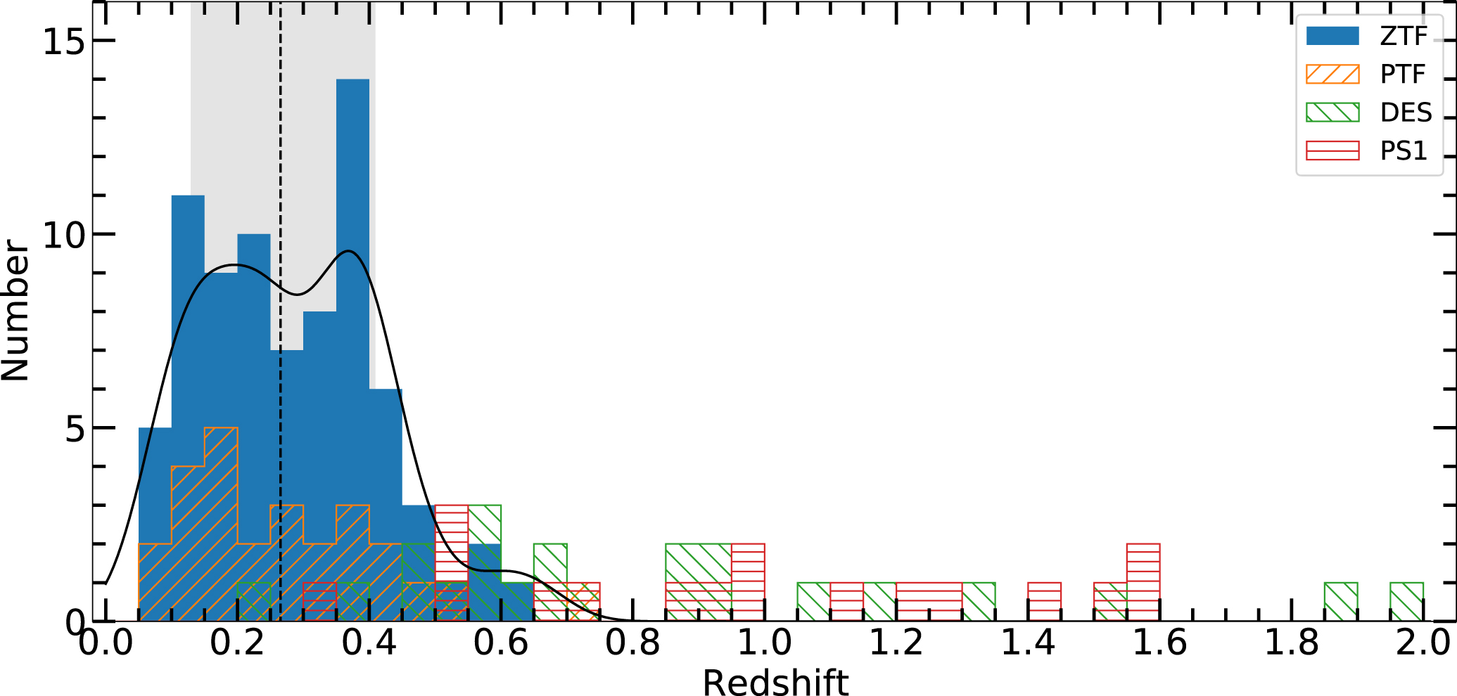
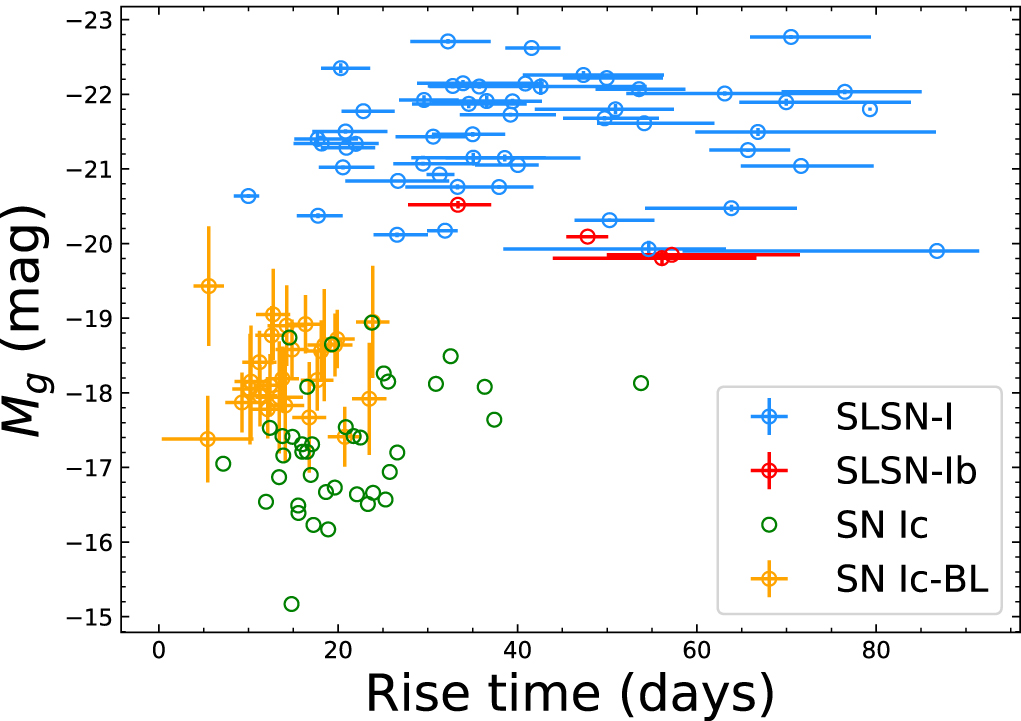
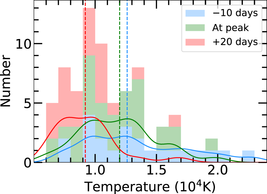
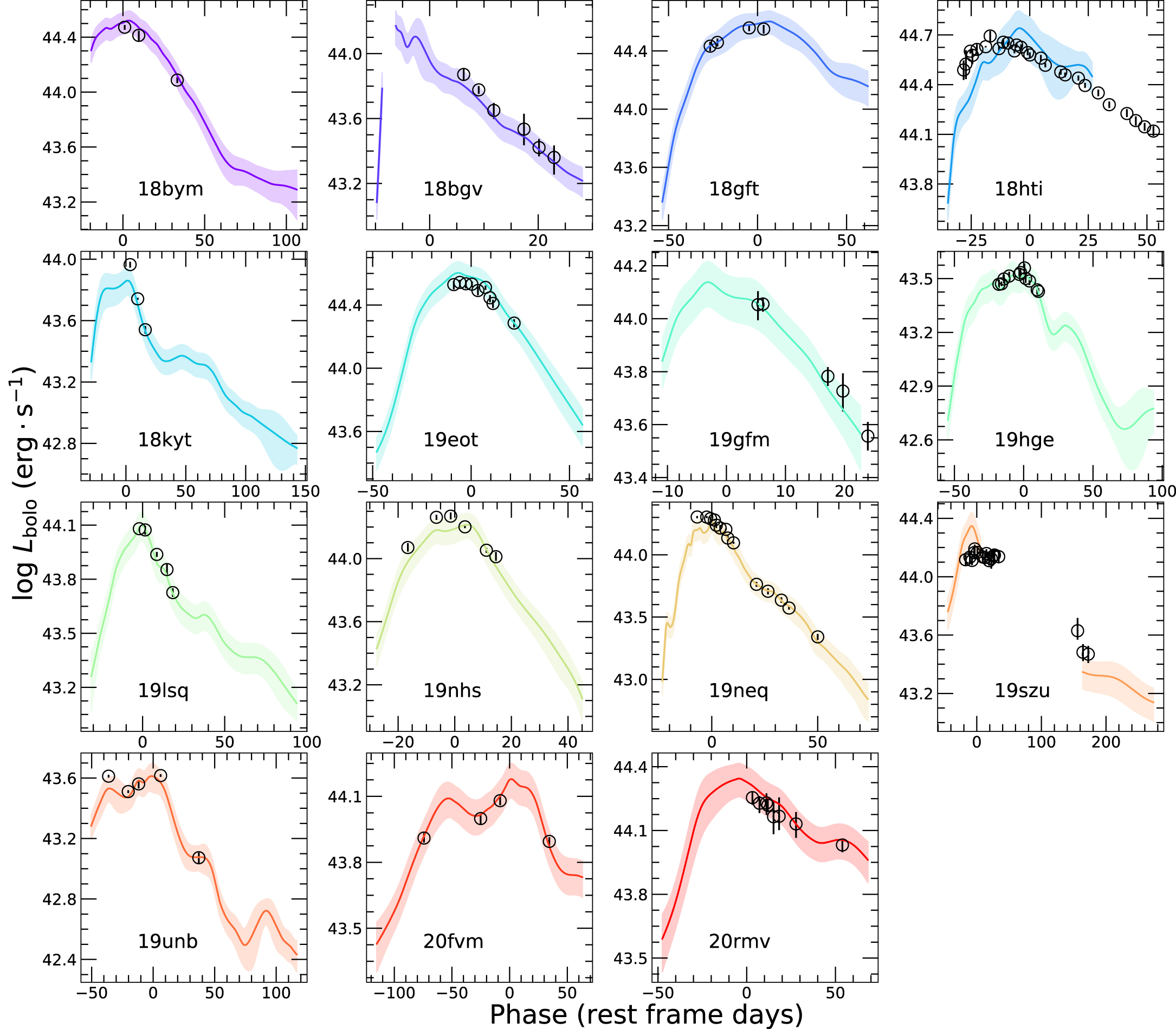
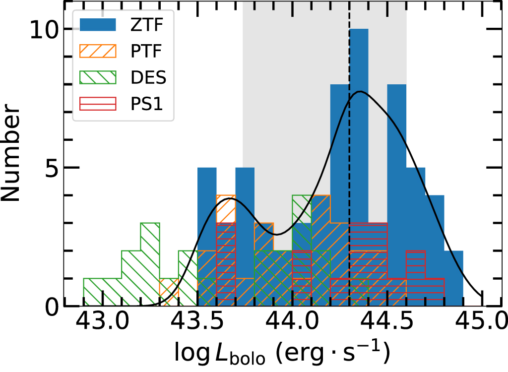
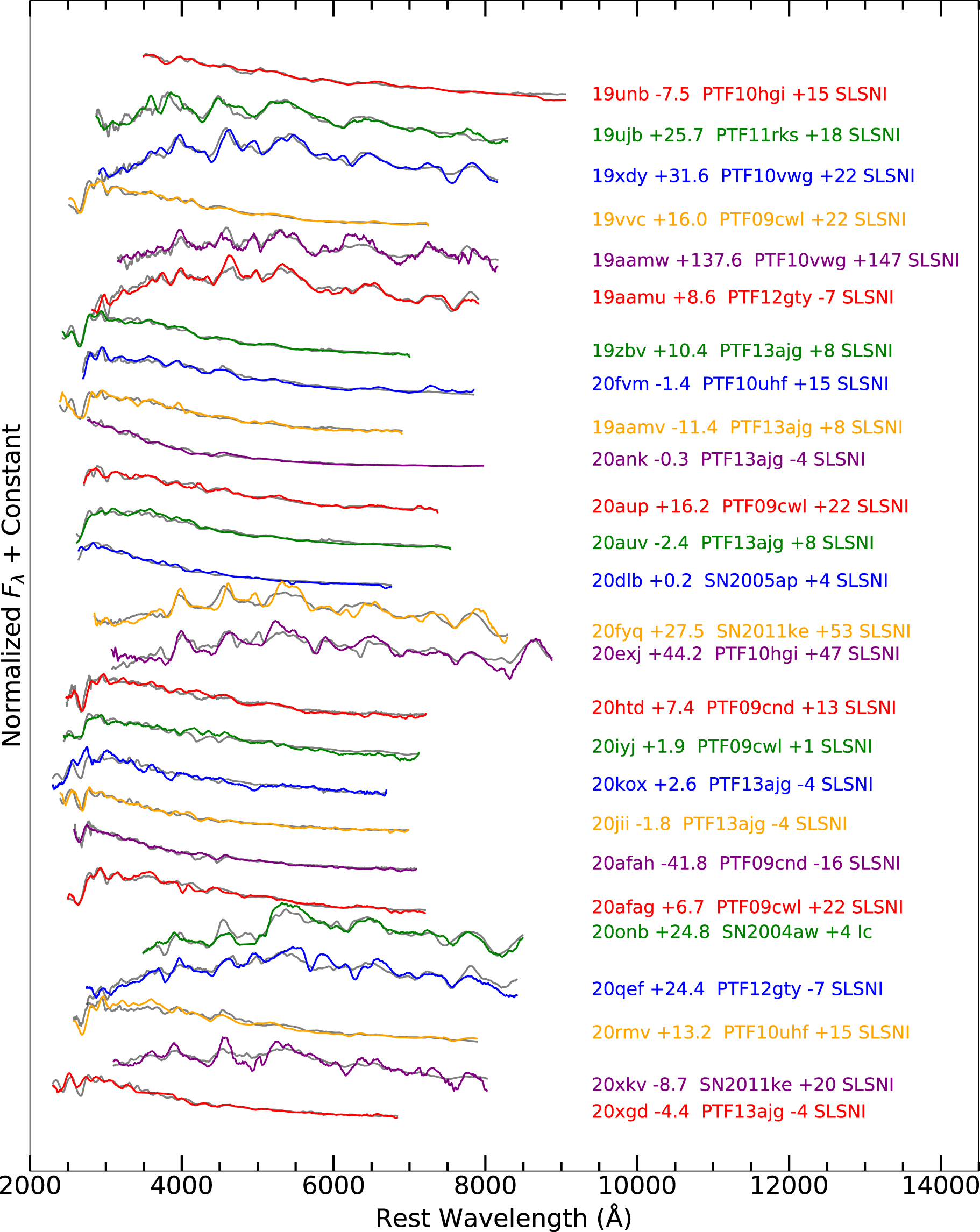
Figure A7. Similar to Figure A2.
Download figure:
Standard image High-resolution image
Table A1. The ZTF SLSN-I Sample
| ZTF Name | IAU Name | R.A. a | Decl. a | Redshift | E(B − V) b | Discovery | Template | Spectrum | Template | Template |
|---|---|---|---|---|---|---|---|---|---|---|
| (mag) | Group | Phase c | Phase c | Type | ||||||
| ZTF18aaisyyp | SN 2018avk | 13:11:27.72 | +65:38:16.7 | 0.132 | 0.011 | Gaia | PTF12gty | −13.5 | −7 | SLSN-I |
| ZTF18aajqcue | SN 2018don | 13:55:08.65 | +58:29:42.0 | 0.0735 | 0.0089 | PS1 | SN2007gr | −2.1 | −7 | Ic |
| ZTF18aapgrxo | SN 2018bym | 18:43:13.42 | +45:12:28.2 | 0.2744 | 0.0517 | ATLAS | PTF13ajg | +5.4 | +8 | SLSN-I |
| ZTF18aavrmcg | SN 2018bgv | 11:02:30.29 | +55:35:55.8 | 0.0795 | 0.0074 | Gaia | SN2011ke | +17.8 | +20 | SLSN-I |
| ZTF18aazgrfl | SN 2018lzv | 12:44:02.32 | +56:01:44.5 | 0.434 | 0.0081 | ZTF | PTF09atu | −19.1 | −20 | SLSN-I |
| ZTF18abjwagv | SN 2018gbw | 15:55:38.02 | +28:21:38.0 | 0.3454 | 0.0386 | PS1 | PTF13ajg | −4.1 | −4 | SLSN-I |
| ZTF18abmasep | SN 2018fcg | 21:09:36.78 | +33:28:59.6 | 0.1011 | 0.1435 | ZTF | PTF12dam | −4.4 | −22 | SLSN-I |
| ZTF18abrzcbp | SN 2018lzw | 07:39:32.76 | +27:44:02.7 | 0.3198 | 0.0373 | ZTF | PTF10uhf | +27.6 | +15 | SLSN-I |
| ZTF18abshezu | SN 2018gft | 23:57:17.95 | −15:37:53.3 | 0.2320 | 0.0256 | ZTF | PTF09cnd | −38.4 | −14 | SLSN-I |
| ZTF18abszecm | SN 2018lzx | 22:29:27.24 | +13:10:39.8 | 0.4373 | 0.0529 | ZTF | PTF09cnd | +19.2 | +37 | SLSN-I |
| ZTF18abvgjyl | SN 2018gkz | 07:58:11.54 | +19:31:07.9 | 0.2405 | 0.036 | ZTF | SN2007bi | +10.6 | +50 | SLSN-I |
| ZTF18acapyww | SN 2018hpq | 18:28:41.24 | +75:48:47.3 | 0.124 | 0.0868 | Gaia | PTF10nmn | +25.0 | max | SLSN-I |
| ZTF18acenqto | SN 2018ibb | 04:38:56.93 | −20:39:44.2 | 0.166 | 0.0275 | ATLAS | PTF12dam | −4.0 | +7 | SLSN-I |
| ZTF18acqyvag | SN 2018lfe | 09:33:29.56 | +00:03:08.4 | 0.3505 | 0.0286 | PS1 | SN2011ke | +59.6 | +53 | SLSN-I |
| ZTF18acslpji | SN 2018hti | 03:40:53.77 | +11:46:37.9 | 0.0613 | 0.3983 | ATLAS | PTF12dam | +21.2 | +7 | SLSN-I |
| ZTF18acxgqxq | SN 2018lfd | 23:14:59.32 | +48:45:27.6 | 0.2686 | 0.1506 | ZTF | PTF12dam | −7.5 | −22 | SLSN-I |
| ZTF18acyxnyw | SN 2018kyt | 12:27:56.23 | +56:23:35.6 | 0.1080 | 0.0091 | ZTF | PTF10hgi | +45.5 | +47 | SLSN-I |
| ZTF19aacxrab | SN 2019J | 10:03:46.78 | +06:46:24.7 | 0.1346 | 0.0229 | PS1 | PTF10gvb | +8.8 | −6 | SLSN-I |
| ZTF19aajwogx | SN 2019cca | 12:02:50.91 | −16:39:53.6 | 0.4103 | 0.0462 | ZTF | PTF10uhf | +28.5 | +15 | SLSN-I |
| ZTF19aaknqmp | SN 2019bgu | 09:57:15.34 | +32:00:05.6 | 0.1480 | 0.0123 | ATLAS | PTF12gty | +16.6 | −7 | SLSN-I |
| ZTF19aalbrph | SN 2019kwq | 17:07:58.84 | +58:42:03.9 | 0.49 d | 0.0257 | ZTF | PTF09cnd | +68.9 | +37 | SLSN-I |
| ZTF19aamhast | SN 2019dgr | 09:45:32.68 | +04:56:02.2 | 0.3815 | 0.0348 | ATLAS | PTF13ajg | +13.2 | +8 | SLSN-I |
| ZTF19aamhhiz | SN 2019kws | 14:15:04.46 | +50:39:06.8 | 0.1977 | 0.0142 | ZTF | PTF12gty | +21.7 | −7 | SLSN-I |
| ZTF19aanesgt | SN 2019cdt | 08:17:53.90 | +65:28:46.7 | 0.153 | 0.0441 | ZTF | PTF10nmn | +11.6 | +29 | SLSN-I |
| ZTF19aantokv | SN 2019aamp | 14:37:49.27 | +20:18:16.6 | 0.4040 | 0.0237 | ZTF | PTF13ajg | +8.4 | +8 | SLSN-I |
| ZTF19aaohuwc | SN 2019dlr | 11:17:34.18 | +00:30:02.6 | 0.26 d | 0.0309 | ZTF | SN2004aw | +57.7 | +11 | Ic |
| ZTF19aapaeye | SN 2019cwu | 14:51:37.29 | +48:59:13.7 | 0.32 d | 0.0186 | ZTF | SN2011ke | +27.6 | +20 | SLSN-I |
| ZTF19aaqrime | SN 2019kwt | 19:39:22.59 | +78:45:43.8 | 0.3562 | 0.0775 | ZTF | SN2007bi | +11.3 | +50 | SLSN-I |
| ZTF19aarphwc | SN 2019eot | 18:00:29.95 | +50:17:43.3 | 0.3057 | 0.0366 | ZTF | PTF13ajg | −13.8 | −4 | SLSN-I |
| ZTF19aaruixj | SN 2019kwu | 13:57:39.77 | +64:21:18.6 | 0.60 d | 0.0138 | ZTF | PTF10vqv | +28.4 | +11 | SLSN-I |
| ZTF19aasdvfr | SN 2019gqi | 14:21:11.98 | +28:54:05.9 | 0.3642 | 0.0129 | ATLAS | PTF11rks | +21.3 | +7 | SLSN-I |
| ZTF19aauiref | SN 2019fiy | 14:05:46.73 | +33:27:38.3 | 0.67 d | 0.0142 | PS1 | PTF09atu | +15.6 | +28 | SLSN-I |
| ZTF19aauvzyh | SN 2019gam | 10:19:18.32 | +17:12:42.6 | 0.1235 | 0.0272 | ATLAS | SN2011ke | +17.6 | +29 | SLSN-I |
| ZTF19aavouyw | SN 2019gfm | 15:35:46.59 | +24:03:45.0 | 0.1816 | 0.0465 | PS1 | PTF11rks | +16.8 | +18 | SLSN-I |
| ZTF19aawfbtg | SN 2019hge | 22:24:21.20 | +24:47:17.1 | 0.0866 | 0.058 | ZTF | PTF12dam | −25.7 | +2 | SLSN-I |
| ZTF19aawsqsc | SN 2019hno | 19:39:12.95 | +62:43:41.0 | 0.26 | 0.0583 | ATLAS | PTF09cnd | +1.6 | +9 | SLSN-I |
| ZTF19aayclnm | SN 2019aamq | 20:55:36.14 | −08:40:31.4 | 0.386 | 0.0636 | ZTF | PTF10bjp | +3.8 | +8 | SLSN-I |
| ZTF19abaeyqw | SN 2019kcy | 14:08:19.78 | +08:58:01.0 | 0.399 | 0.0227 | ZTF | PTF13ajg | −19.3 | −4 | SLSN-I |
| ZTF19abcvwrz | SN 2019aamx | 15:57:48.27 | +27:28:03.5 | 0.41 | 0.0362 | ZTF | PTF09cwl | +13.0 | +22 | SLSN-I |
| ZTF19abdlzyq | SN 2019aamr | 15:29:23.55 | +38:06:12.6 | 0.42 d | 0.0118 | ZTF | PTF09cwl | +8.0 | +22 | SLSN-I |
| ZTF19abfvnns | SN 2019lsq | 00:04:40.58 | +42:52:11.3 | 0.1295 | 0.0829 | ATLAS | PTF12dam | −3.3 | −22 | SLSN-I |
| ZTF19abkfshj | SN 2019otl | 02:52:21.63 | −17:48:12.4 | 0.500 | 0.0241 | ZTF | PTF13ajg | +11.2 | −4 | SLSN-I |
| ZTF19abnacvf | SN 2019nhs | 00:52:01.44 | +07:36:59.7 | 0.189 | 0.0514 | PS1 | PTF13ajg | −8.6 | −4 | SLSN-I |
| ZTF19abnqqdp | SN 2019aams | 23:43:36.16 | +12:29:01.0 | 0.6360 | 0.0448 | ZTF | PTF13ajg | +0.8 | −4 | SLSN-I |
| ZTF19abpbopt | SN 2019neq | 17:54:26.76 | +47:15:40.6 | 0.1060 | 0.0334 | ZTF | PTF11rks | +16.1 | +7 | SLSN-I |
| ZTF19abrbsvm | SN 2019obk | 22:33:54.08 | −02:09:42.3 | 0.1656 | 0.048 | PS1 | PTF12gty | +12.8 | −7 | SLSN-I |
| ZTF19abuolvj | SN 2019qgk | 22:29:57.55 | −04:06:02.2 | 0.3468 | 0.054 | ZTF | SN2010gx | +47.2 | +29 | SLSN-I |
| ZTF19abuyuwa | SN 2019sgg | 01:01:11.77 | +14:01:35.4 | 0.5726 | 0.0373 | ZTF | PTF13ajg | −18.6 | −4 | SLSN-I |
| ZTF19abzoyeg | SN 2019aamt | 21:15:08.00 | +32:43:01.3 | 0.2138 | 0.126 | ZTF | PTF12dam | +15.2 | +7 | SLSN-I |
| ZTF19abzqmau | SN 2019sgh | 01:12:39.42 | +36:28:24.8 | 0.3436 | 0.0599 | ZTF | PTF10uhf | +39.8 | +15 | SLSN-I |
| ZTF19acbonaa | SN 2019stc | 06:54:23.10 | +17:29:31.4 | 0.1178 | 0.072 | ZTF | PTF10hgi | +25.6 | +47 | SLSN-I |
| ZTF19acfwynw | SN 2019szu | 00:10:13.14 | −19:41:32.4 | 0.2120 | 0.018 | ATLAS | PTF12dam | −15.2 | +2 | SLSN-I |
| ZTF19acgjpgh | SN 2019unb | 09:47:57.02 | +00:49:36.0 | 0.0635 | 0.1045 | ZTF | PTF10hgi | −7.5 | +15 | SLSN-I |
| ZTF19ackjrru | SN 2019ujb | 09:03:15.18 | +40:14:32.6 | 0.2008 | 0.0165 | ZTF | PTF11rks | +25.7 | +18 | SLSN-I |
| ZTF19acsajxn | SN 2019xdy | 08:24:51.33 | +22:10:46.0 | 0.2206 | 0.0425 | ZTF | PTF10vwg | +31.6 | +22 | SLSN-I |
| ZTF19acucxij | SN 2019vvc | 09:13:30.13 | +44:46:26.2 | 0.3314 | 0.0115 | ATLAS | PTF09cwl | +16.0 | +22 | SLSN-I |
| ZTF19acvxquk | SN 2019aamu | 02:55:08.89 | +11:27:22.4 | 0.2590 | 0.1925 | ZTF | PTF12gty | +8.6 | −7 | SLSN-I |
| ZTF19adaivcf | SN 2019zbv | 10:15:01.10 | +43:24:53.6 | 0.3785 | 0.0119 | ZTF | PTF13ajg | +10.4 | +8 | SLSN-I |
| ZTF20aahbfmf | SN 2020ank | 08:16:14.65 | +04:19:26.9 | 0.2485 | 0.0193 | ZTF | PTF13ajg | −0.3 | −4 | SLSN-I |
| ZTF20aaifybu | SN 2020auv | 16:34:12.51 | +13:05:51.9 | 0.280 | 0.0565 | ZTF | PTF13ajg | −2.4 | +8 | SLSN-I |
| ZTF19acujvsi | SN 2019aamw | 23:48:54.54 | +24:59:59.8 | 0.22 d | 0.0526 | ZTF | PTF10vwg | +137.6 | +147 | SLSN-I |
| ZTF20aadzbcf | SN 2020fvm | 14:12:45.93 | +34:44:16.2 | 0.2428 | 0.0129 | ZTF | PTF10uhf | −1.4 | +15 | SLSN-I |
| ZTF20aagikvv | SN 2019aamv | 12:45:01.65 | +33:33:14.1 | 0.3996 | 0.0127 | ZTF | PTF13ajg | −11.4 | +8 | SLSN-I |
| ZTF20aahrxgw | SN 2020aup | 13:09:44.44 | +12:29:13.4 | 0.31 d | 0.0208 | ZTF | PTF09cwl | +16.2 | +22 | SLSN-I |
| ZTF20aaoqwpo | SN 2020dlb | 08:08:34.14 | +34:44:12.9 | 0.398 | 0.0327 | ZTF | SN2005ap | +0.2 | +4 | SLSN-I |
| ZTF20aapaecd | SN 2020fyq | 14:46:10.44 | +23:48:02.0 | 0.1765 | 0.0325 | PS1 | SN2011ke | +27.5 | +53 | SLSN-I |
| ZTF20aattyuz | SN 2020exj | 14:42:40.01 | +30:14:39.1 | 0.1216 | 0.0096 | ATLAS | PTF10hgi | +44.2 | +47 | SLSN-I |
| ZTF20aauoudz | SN 2020htd | 17:44:17.28 | +38:55:30.4 | 0.3515 | 0.026 | PS1 | PTF09cnd | +7.4 | +13 | SLSN-I |
| ZTF20aavfbqz | SN 2020iyj | 09:15:36.64 | +53:27:32.0 | 0.3690 | 0.0155 | ZTF | PTF09cwl | +1.9 | +1 | SLSN-I |
| ZTF20aavqrzc | SN 2020kox | 11:06:04.97 | +26:17:28.7 | 0.456 | 0.0166 | ATLAS | PTF13ajg | +2.6 | −4 | SLSN-I |
| ZTF20aawfxlt | SN 2020jii | 15:34:55.31 | +02:51:11.5 | 0.396 | 0.0427 | PS1 | PTF13ajg | −1.8 | −4 | SLSN-I |
| ZTF20aawkgxa | SN 2020afah | 10:20:18.32 | +53:19:21.4 | 0.3754 | 0.0086 | ZTF | PTF09cnd | −41.8 | −16 | SLSN-I |
| ZTF20abisijg | SN 2020afag | 00:15:46.25 | +47:00:08.5 | 0.3815 | 0.0898 | ZTF | PTF09cwl | +6.7 | +22 | SLSN-I |
| ZTF20abjwjrx | SN 2020onb | 14:23:00.61 | +49:10:40.7 | 0.16 d | 0.0208 | ZTF | SN2004aw | +24.8 | +4 | Ic |
| ZTF20ablkuio | SN 2020qef | 22:56:10.53 | +28:45:53.3 | 0.1831 | 0.0459 | ATLAS | PTF12gty | +24.4 | −7 | SLSN-I |
| ZTF20abpuwxl | SN 2020rmv | 00:40:00.19 | −14:35:25.1 | 0.2621 | 0.0185 | ATLAS | PTF10uhf | +13.2 | +15 | SLSN-I |
| ZTF20abzaacf | SN 2020xkv | 22:37:46.00 | +23:31:37.4 | 0.2410 | 0.0303 | ATLAS | SN2011ke | −8.7 | +20 | SLSN-I |
| ZTF20aceqspy | SN 2020xgd | 00:19:45.83 | +05:08:18.7 | 0.455 | 0.0145 | PS1 | PTF13ajg | −4.4 | −4 | SLSN-I |
Notes.
a In J2000. b From Schlafly & Finkbeiner (2011). c In rest-frame days. d This means that the redshift is fit by superfit.A machine-readable version of the table is available.
Table A2. Classification Spectra
| Name | Observing Date | Telescope + Instrument | Exposure Time a (s) |
|---|---|---|---|
| SN 2018avk | 2018-5-4 | NOT+ALFOSC | 1800 |
| SN 2018don | 2018-6-9 | P200+DBSP | 2 × 600/2 × 600 |
| SN 2018bym | 2018-6-12 | P200+DBSP | 600/600 |
| SN 2018bgv | 2018-6-4 | NOT+ALFOSC | 2 × 2400 |
| SN 2018lzv | 2018-7-14 | WHT+ISIS | 600 |
| SN 2018gbw | 2018-8-13 | P200+DBSP | 600/600 |
| SN 2018fcg | 2018-8-21 | P200+DBSP | 600/600 |
| SN 2018lzw | 2018-10-6 | P200+DBSP | 610/400 |
Notes. (This table is available in its entirety in machine-readable form.)
a The slash-separated values indicate the exposure times of the blue and red sides, respectively.Only a portion of this table is shown here to demonstrate its form and content. A machine-readable version of the full table is available.
Download table as: DataTypeset image
Table A3. Photometry Data
| Name | MJD | Filter | Mag(AB) | Errormag | Label a | Fluxratio b | Tel.+Ins. c |
|---|---|---|---|---|---|---|---|
| (days) | (mag) | (mag) | (10−9) | ||||
| SN 2018avk | 58202.30 | g | 20.48 | 0.21 | F | 6.40 | P48+ZTF |
| SN 2018avk | 58202.32 | g | 20.64 | 0.18 | F | 5.53 | P48+ZTF |
| SN 2018avk | 58202.32 | g | 20.74 | 0.16 | F | 5.04 | P48+ZTF |
| SN 2018avk | 58202.34 | g | 20.78 | 0.19 | F | 4.86 | P48+ZTF |
| SN 2018avk | 58202.36 | g | 20.92 | 0.14 | F | 4.27 | P48+ZTF |
| SN 2018avk | 58202.36 | g | 20.80 | 0.21 | F | 4.77 | P48+ZTF |
| SN 2018avk | 58203.35 | g | 20.54 | 0.15 | F | 6.06 | P48+ZTF |
| SN 2018avk | 58204.39 | g | 20.10 | 0.19 | F | 9.09 | P48+ZTF |
Notes. (This table is available in its entirety in machine-readable form.)
a F means real detection and T means upper limit. b The ratio of the observed flux and the flux zeropoint. c Telescope + Instrument.Only a portion of this table is shown here to demonstrate its form and content. A machine-readable version of the full table is available.
Download table as: DataTypeset image
Table A4. LC Properties
| Name | K-correction a | Mpeak | Lpeak | tpeak | trise,1/e | tdecay,1/e | trise,10% |
|---|---|---|---|---|---|---|---|
| (mag) | (mag) | (1043 erg s−1) | (MJD) | (days) | (days) | (days) | |
| SN 2018avk | −0.00 | −20.31 ± 0.02 | 5.5 ± 1.0 |

|

|

|

|
| SN 2018don | 0.09 | −20.06 ± 0.01 | 3.4 ± 0.6 |

|

|

| ⋯ |
| SN 2018bym | −0.22 | −22.04 ± 0.01 | 33.2 ± 5.9 |

|

|

| ⋯ |
| SN 2018bgv | −0.09 | −20.64 ± 0.02 | (14.9 ± 3.6) b |

|

|

|

|
| SN 2018lzv | −0.39 | −22.26 ± 0.05 | 52.6 ± 16.1 |

|

|

|

|
| SN 2018gbw | −0.33 | −22.11 ± 0.03 | (41.1 ± 7.6) |

|

| ⋯ |

|
| SN 2018fcg | −0.13 | −20.37 ± 0.03 | (6.0 ± 1.1) |

|

|

|

|
| SN 2018lzw | −0.30 d | (−21.75 ± 0.05) | (22.7 ± 4.6) | ( ) ) | ⋯ | ( ) ) | ⋯ |
| SN 2018gft | −0.18 | −22.22 ± 0.02 | 40.1 ± 7.2 |

|

| ⋯ |

|
| SN 2018lzx | −0.44 | −22.03 ± 0.03 | 32.6 ± 5.9 |

|

|

|

|
| SN 2018gkz | −0.24 | (−-21.79 ± 0.01) | (21.3 ± 4.3) | ( ) ) | ⋯ | ( ) ) | ⋯ |
| SN 2018hpq | −0.13 d | −20.17 ± 0.02 | 4.8 ± 0.9 |

|

| ⋯ |

|
| SN 2018lfe | −0.33 d | −21.52 ± 0.05 | 27.4 ± 9.1 |

|

|

| ⋯ |
| SN 2018hti | −0.09 | −22.10 ± 0.03 | 55.1 ± 14.9 |

|

| ⋯ |

|
| SN 2018lfd | −0.19 | −21.98 ± 0.07 | 38.6 ± 8.5 |

|

| ⋯ | ⋯ |
| SN 2018kyt | −0.13 | −20.52 ± 0.05 | 9.2 ± 0.4 e |

|

|

|

|
| SN 2019J | −0.05 | −19.93 ± 0.11 | 3.7 ± 0.9 |

|

|

|

|
| SN 2019cca | −0.37 d | −22.02 ± 0.08 | (33.3 ± 7.8) |

|

|

| ⋯ |
| SN 2019bgu | −0.14 | −20.34 ± 0.12 | 5.5 ± 1.4 |

| ⋯ |

| ⋯ |
| SN 2019kwq | −0.43 d | −22.01 ± 0.03 | 32.2 ± 5.8 |

|

|

|

|
| SN 2019dgr | −0.37 | −21.91 ± 0.07 | 33.0 ± 9.8 |

|

| ⋯ |

|
| SN 2019kws | −0.31 | −20.06 ± 0.02 | 5.1 ± 0.9 |

|

|

| ⋯ |
| SN 2019cdt | −0.04 | −20.84 ± 0.02 | 7.6 ± 1.4 |

|

|

|

|
| SN 2019aamp | −0.40 | −21.90 ± 0.03 | 30.5 ± 5.7 |

| ⋯ |

| ⋯ |
| SN 2019dlr | −0.24 | −21.15 ± 0.04 | 18.1 ± 3.7 |

|

|

|

|
| SN 2019cwu | −0.30 | −21.28 ± 0.02 | 17.8 ± 3.4 |

|

|

|

|
| SN 2019kwt | −0.34 | −22.77 ± 0.03 | 65.1 ± 11.9 |

|

|

|

|
| SN 2019eot | −0.28 | −22.14 ± 0.01 | 40.1 ± 7.1 |

|

|

|

|
| SN 2019kwu | −0.51 d | −22.35 ± 0.07 | 50.8 ± 9.4 |

|

|

|

|
| SN 2019gqi | −0.34 d | −21.46 ± 0.03 | 19.3 ± 4.8 |

|

| ⋯ |

|
| SN 2019fiy | −0.69 | −22.71 ± 0.03 | ⋯ |

|

| ⋯ |

|
| SN 2019gam | 0.32 | (−19.92 ± 0.11) | (2.6 ± 0.7) | ( ) ) | ( ) ) | ⋯ | ( ) ) |
| SN 2019gfm | −0.02 | −21.02 ± 0.03 | 13.7 ± 2.7 |

|

|

|

|
| SN 2019hge | −0.11 | −19.85 ± 0.02 | 3.6 ± 0.2 e |

|

|

|

|
| SN 2019hno | −0.21 | −21.07 ± 0.02 | 13.4 ± 2.5 |

|

|

|

|
| SN 2019aamq | −0.36 | −21.78 ± 0.02 | 32.9 ± 11.8 |

|

| ⋯ | ⋯ |
| SN 2019kcy | −0.41 | −22.10 ± 0.11 | 46.6 ± 11.8 |

|

| ⋯ |

|
| SN 2019aamx | −0.33 | −21.80 ± 0.07 | 21.7 ± 4.8 |

|

|

|

|
| SN 2019aamr | −0.41 | −21.40 ± 0.09 | 20.5 ± 4.3 |

|

|

|

|
| SN 2019lsq | −0.22 | −20.92 ± 0.01 | 12.5 ± 2.3 |

|

|

|

|
| SN 2019otl | −0.46 | −22.39 ± 0.04 | (61.2 ± 14.4) |

| ⋯ | − | ⋯ |
| SN 2019nhs | −0.05 | −21.43 ± 0.03 | 18.6 ± 0.9 e |

|

|

|

|
| SN 2019aams | −0.60 | −22.15 ± 0.04 | (47.2 ± 13.6) |

|

|

|

|
| SN 2019neq | −0.24 | −21.34 ± 0.01 | 20.1 ± 0.4 e |

|

|

|

|
| SN 2019obk | −0.10 | −19.80 ± 0.08 | 3.8 ± 1.1 |

|

| ⋯ |

|
| SN 2019qgk | −0.32 d | (−21.58 ± 0.08) | (21.2 ± 5.5) | ( ) ) | ⋯ | ( ) ) | ⋯ |
| SN 2019sgg | −0.42 | (−22.34 ± 0.05) | 56.6 ± 12.0 | ( ) ) | ( ) ) | ⋯ | ( ) ) |
| SN 2019aamt | −0.24 | −20.76 ± 0.03 | 17.0 ± 7.1 |

|

| ⋯ |

|
| SN 2019sgh | −0.34 | −21.34 ± 0.02 | 19.3 ± 3.5 |

|

|

|

|
| SN 2019stc | −0.02 | −20.56 ± 0.03 | 5.8 ± 1.0 |

|

|

| ⋯ |
| SN 2019szu | −0.06 | −21.23 ± 0.05 | 22.3 ± 5.2 |

|

| ⋯ | ⋯ |
| SN 2019unb | −0.03 | −20.13 ± 0.05 | 4.1 ± 0.1 e |

| ⋯ |

| ⋯ |
| SN 2019ujb | −0.05 | −21.15 ± 0.06 | 12.2 ± 2.6 |

|

|

|

|
| SN 2019xdy | −0.22 d | −20.76 ± 0.02 | 7.9 ± 4.2 |

|

|

|

|
| SN 2019vvc | −0.31 d | −22.07 ± 0.03 | 44.7 ± 18.1 |

|

| ⋯ |

|
| SN 2019aamu | −0.25 d | (−21.63 ± 0.09) | ⋯ | ( ) ) | ( ) ) | ⋯ | ( ) ) |
| SN 2019zbv | −0.39 | −22.01 ± 0.02 | 33.4 ± 6.0 |

|

|

| ⋯ |
| SN 2020ank | −0.22 | −21.77 ± 0.02 | 24.6 ± 4.5 |

|

|

|

|
| SN 2020auv | −0.21 | −21.87 ± 0.05 | 31.2 ± 6.7 |

| ⋯ |

| ⋯ |
| SN 2019aamw | −0.22 d | −20.47 ± 0.04 | 6.4 ± 1.3 |

|

|

|

|
| SN 2020fvm | −0.19 | −21.42 ± 0.02 | 15.1 ± 2.7 |

|
 c
c
| ⋯ | ⋯ |
| SN 2019aamv | −0.38 | −21.50 ± 0.05 | 19.6 ± 3.9 |

|

|

|

|
| SN 2020aup | −0.28 | −21.50 ± 0.03 | 24.6 ± 4.8 |

|

|

|

|
| SN 2020dlb | −0.36 d | −22.62 ± 0.03 | 78.0 ± 23.9 |

|

|

|

|
| SN 2020fyq | −0.18 d | −19.90 ± 0.02 | 3.2 ± 0.6 |

|

|

|

|
| SN 2020exj | −0.22 | −20.12 ± 0.03 | 5.2 ± 1.0 |

|

|

|

|
| SN 2020htd | −0.33 d | −21.25 ± 0.02 | 14.3 ± 2.6 |

|

|

|

|
| SN 2020iyj | −0.35 | −21.73 ± 0.03 | 23.3 ± 4.3 |

|

|

|

|
| SN 2020kox | −0.36 | −21.87 ± 0.06 | (44.6 ± 12.7) |

|

| ⋯ |

|
| SN 2020jii | −0.40 | −21.91 ± 0.03 | 44.2 ± 13.9 |

|

|

|

|
| SN 2020afah | −0.35 d | −21.89 ± 0.05 | 25.0 ± 5.3 |

|

|

|

|
| SN 2020afag | −0.37 | −21.68 ± 0.03 | 23.6 ± 4.3 |

|

|

|

|
| SN 2020onb | −0.11 | −21.05 ± 0.02 | 9.8 ± 1.8 |

|

| ⋯ |

|
| SN 2020qef | −0.26 | −20.09 ± 0.02 | 4.3 ± 0.8 |

|

|

|

|
| SN 2020rmv | −0.18 | −21.61 ± 0.02 | 22.1 ± 3.9 |

|

| ⋯ |

|
| SN 2020xkv | −0.36 | −21.04 ± 0.02 | 10.7 ± 2.0 |

|

| ⋯ |

|
| SN 2020xgd | −0.45 | −21.92 ± 0.06 | 34.7 ± 6.7 |

|

|

|

|
Notes. Mpeak, tpeak, trise,1/e, tdecay,1/e, and trise,10% are measured in the rest-frame g-band LCs.
a The K-correction to the rest-frame g-band at the peak. It equals Kg→g for z ≤ 0.17 and Kr→g for z > 0.17. b The values in parentheses mean that the values are not well constrained due to the lack of data. c SN 2020fvm has two LC peaks and its trise,1/e is days, if the first (and the fainter) one is set as the main peak.
d
This means that the K-correction is calculated by
days, if the first (and the fainter) one is set as the main peak.
d
This means that the K-correction is calculated by  .
e
This means that the Lpeak is calculated from multiband data, instead of corrected from the g- and r-band flux.
.
e
This means that the Lpeak is calculated from multiband data, instead of corrected from the g- and r-band flux.
A machine-readable version of the table is available.
Table A5. (g − r) Colors at the Peak
| Name | Observed | Rest Frame |
|---|---|---|
| (mag) | (mag) | |
| SN 2018avk | −0.03 ± 0.03 | −0.21 ± 0.03 |
| SN 2018don | 0.15 ± 0.02 | −0.01 ± 0.02 |
| SN 2018bym | −0.11 ± 0.01 | −0.32 ± 0.06 |
| SN 2018bgv | −0.23 ± 0.03 | −0.25 ± 0.03 |
| SN 2018lzv | −0.03 ± 0.07 | ⋯ |
| SN 2018gbw | −0.12 ± 0.04 | ⋯ |
| SN 2018fcg | −0.16 ± 0.04 | −0.18 ± 0.04 |
| SN 2018gft | −0.14 ± 0.03 | −0.21 ± 0.05 |
| SN 2018lzx | 0.02 ± 0.04 | ⋯ |
| SN 2018hpq | −0.11 ± 0.02 | ⋯ |
Only a portion of this table is shown here to demonstrate its form and content. A machine-readable version of the full table is available.
Download table as: DataTypeset image
Table A6. Temperatures and Bolometric Luminosities
| Name | Phase | Temperature | Lbolo | Radius |
|---|---|---|---|---|
| (days) | (104 K) | (1043 erg s−1) | (1010 km) | |
| SN 2018avk | −4.23 |

|

|

|
| SN 2018avk | 16.97 |

|

|

|
| SN 2018bym | 1.06 |

|

|

|
| SN 2018bym | 9.70 |

|

|

|
| SN 2018bym | 33.24 |

|

|

|
| SN 2018bgv | 6.26 |

|

|

|
| SN 2018bgv | 9.04 |

|

|

|
| SN 2018bgv | 11.82 |

|

|

|
| SN 2018bgv | 17.38 |

|

|

|
| SN 2018bgv | 20.16 |

|

|

|
| SN 2018bgv | 22.94 |

|

|

|
Only a portion of this table is shown here to demonstrate its form and content. A machine-readable version of the full table is available.
Download table as: DataTypeset image
Footnotes
- 26
The ZTF public survey transitioned to a 2 day cadence on 2020 October 1, but the official start of the ZTF Phase II is 2020 December 1. We picked our date range for the convenience of the sources analyzed in our sample.
- 27
- 28
- 29
- 30
- 31
- 32
Another definition of BC is Mbolo = MK + BCK for the K-band absolute magnitude MK , where Mbolo is the bolometric magnitude. Our correction is applied to two bands (g and r), and we use the definition introduced in Section 5.3.