


Abstract
We analyze the formation and three-dimensional (3D) evolution of two coronal mass ejections (CMEs) and their associated waves in the low corona via a detailed multi-viewpoint analysis of extreme-ultraviolet observations. We analyze the kinematics in the radial and lateral directions and identify three stages in the early evolution of the CME: (1) a hyper-inflation stage, when the CME laterally expands at speeds of ∼1000 km s−1, followed by (2) a shorter and slower expansion stage of a few minutes and ending with (3) a self-similar phase that carries the CME into the middle corona. The first two stages coincide with the impulsive phase of the accompanying flare, the formation and separation of an EUV wave from the CME, and the start of the metric type II radio burst. Our 3D analysis suggests that the hyper-inflation phase may be a crucial stage in the CME formation with wide-ranging implications for solar eruption research. It likely represents the formation stage of the magnetic structure that is eventually ejected into the corona, as the white-light CME. It appears to be driven by the injection of poloidal flux into the ejecting magnetic structure, which leads to the lateral (primarily) growth of the magnetic flux rope. The rapid growth results in the creation of EUV waves and eventually shocks at the CME flanks that are detected as metric type II radio bursts. In other words, the hyper-inflation stage in the early CME evolution may be the "missing" link between CMEs, flares, and coronal shocks.
Export citation and abstract BibTeX RIS

Original content from this work may be used under the terms of the Creative Commons Attribution 4.0 licence. Any further distribution of this work must maintain attribution to the author(s) and the title of the work, journal citation and DOI.
1. Introduction
Coronal mass ejections (CMEs) are the primary manifestation of explosive energy release processes on the Sun. Observations by space-borne white-light coronagraphs and extreme-ultraviolet (EUV) imagers have largely established the average physical properties of CMEs (Vourlidas et al. 2010); their connection to other energetic phenomena, such as flares, erupting prominences, and solar energetic particle (SEP) events (Webb & Howard 2012); and their central role as drivers of space weather (Temmer 2021).
The kinematic profiles of these events have been a major focus of research, as they hold clues about the eruption processes that drive CMEs by transforming magnetic into kinetic energy and about the potential effects of the event on space weather (Temmer 2016). Fast CMEs can drive coronal (and inner heliospheric) shocks that accelerate high-energy SEPs that pose a direct threat to space assets and human exploration (Temmer 2021).
Numerous analyses (e.g., Zhang et al. 2004) have established a three-phase paradigm for the CME kinetic profile in the corona (at heliocentric distances ≤30 R⊙). Namely, a slow rise (lasting from minutes to several hours to days, even) is followed by a sharp but generally short (∼minutes) acceleration phase, culminating in a usually constant speed phase. Events faster (slower) than the ambient solar wind tend to decelerate (accelerate) during the third phase. The process seems to continue beyond the typical coronagraph field of view of 15–30 R⊙, resulting in fast (slow) CMEs reaching Earth with lower (faster) speeds than their coronal speeds (e.g., Gopalswamy et al. 2000).
While this kinematic profile holds true for hundreds of CMEs, it is based on measurements of a single point (the CME front, namely, the fastest point of the event) made mostly from a single viewpoint. The sharp acceleration phase occurs below 2–3 R⊙, even lower for the fastest CMEs. However, this height range is difficult to observe because it lies at the transition from the EUV to the white-light coverage, the CME is still small, and significant foreground and background structure exists. As a result, relatively little is known about the three-dimensional (3D) evolution of CMEs below 3 R⊙. This is also the region where CME-driven waves (or shocks) develop, confusing further the analysis of the CME envelope and hindering our understanding of particle acceleration (e.g., Vourlidas 2021).
From the early comparisons of the CME size in the low EUV with the Extreme-Ultraviolet Imaging Telescope (EIT; Delaboudinière et al. 1995) and middle white-light corona with the Large Angle and Spectrometric Coronagraph (LASCO; Brueckner et al. 1995), both instruments on the Solar and Heliospheric Observatory (SOHO; Domingo et al. 1995) spacecraft, it became apparent that CMEs must expand asymmetrically in the low (EUV) corona to match the widths observed in the coronagraph field of view. This asymmetric expansion in the lateral direction was first noted by Zhang et al. (2004), who deduced scales of the order of 30–50 minutes for the duration of this non-self-similar phase. The asymmetric expansion contrasts with the largely self-similar expansion that characterizes the grand majority of CMEs in the middle-outer corona (e.g., Balmaceda et al. 2020, and references therein), suggesting that different mechanisms may be at play during the formation and initial acceleration of CMEs. However, the single viewpoint, low cadence (∼12 minutes), and coverage gap between the EIT and LASCO measurements prevented any detailed analysis of the expansion profile of CMEs in the low corona.
This is no longer true since the advent of multi-viewpoint EUV and white-light observations with the instruments of the Sun Earth Connection Coronal and Heliospheric Investigation suite (SECCHI, Howard et al. 2008) from the Solar Terrestrial Relations Observatory (STEREO; Kaiser et al. 2008) and from near-Earth orbits. The multi-viewpoint analysis can provide deprojected kinematic measurements of the CME front height, as well as its lateral size, not only for the CME but also for the associated shock wave. These analyses revealed a much different picture for the early CME expansion profile (Cremades et al. 2020).
Patsourakos et al. (2010a) showed that CMEs can reach expansion speeds of up to 1000 km s−1 in the low corona within just 5–6 minutes, a time interval too short to be detected by previous instrumentation. This was later confirmed by Olmedo et al. (2012) and Cheng et al. (2013) analyzing high-cadence data from the Atmospheric Imaging Assembly (AIA; Lemen et al. 2012) on the Solar Dynamics Observatory (SDO; Pesnell et al. 2012). It is becoming clear, therefore, that the acceleration phase of CMEs (derived from measurements of the CME front height) is connected with a "super-expansion" phase parallel to the solar surface. We define this phase as the hyper-inflation phase to express the asymmetric increase in the CME volume. The deduced speeds are sufficiently high to drive strong shocks in the low corona, which in turn can lead to energetic particle acceleration. The short duration of the hyper-inflation phase explains why it was not recognized in earlier studies. Most importantly, the characteristics of the hyper-inflation phase provide a way to connect CMEs, flares, and SEPs into a coherent picture (Patsourakos & Vourlidas 2012).
Working toward the completion of this picture is the goal of the present paper. We select two impulsive CMEs, both associated with SEPs (>25 MeV protons detected at Earth) and analyze in great detail their 3D formation and kinematic profile in the low corona, including the accompanying waves to assess the role of shock acceleration in the presence or not of SEPs. We take advantage of the multi-viewpoint, high-resolution, high-cadence observations from STEREO and SDO. Our objective is the characterization of the hyper-inflation phase of the two events and their relation to the wave formation.
The paper is organized as follows. Section 2 presents the observations and our methodology for the 3D reconstruction of the event size and kinematics. The events are described in Section 3. The results on the 3D kinematic evolution of the CME and the associated wave are presented in Section 4. We discuss these results and their implications for the flare–CME–shock paradigm in Section 5 and conclude in Section 6.
2. Methodology
2.1. Data and Event Selection
The two CMEs analyzed here were selected because they exhibited a bubble-like appearance in the EUV. An EUV "bubble" is a spherical-like dark (in the EUV) structure surrounded by a bright rim (first noted by Dere et al. 1997). As discussed in Patsourakos et al. (2010a), such structures are the low coronal counterpart of the white-light CME cavity and are strong indications of an impulsive event (i.e., events that exhibit a rapid acceleration low in the corona). Bubble-like CMEs are, hence, primary candidates for hyper-inflation studies. The two CMEs occurred on 2011 March 7 and 2011 June 7.
Both events were observed near simultaneously from different vantage points with the best available temporal cadence. This allows us to derive the low coronal 3D kinematics and volume of the expanding structures in great detail. We use images from AIA on board SDO and from the Extreme Ultra-Violet Imager (EUVI) on board STEREO-A/B. We select images in the EUV channels in which waves are best observed: 195 Å (EUVI) and 193, 211, and 335 Å (AIA). These channels capture plasmas with peak response temperatures in the range 1.0–2.5 MK (O'Dwyer et al. 2010). For the events analyzed here, the AIA data have a 12 s temporal cadence, while the EUVI data are acquired at 2.5- and 5-minute cadence for STA and STB, respectively. To better identify and distinguish the wave and the driver features, we use wavelet-processed images with the technique described by Stenborg et al. (2008) that brings out the fainter EUV structures. Fits files for the wavelet-processed EUVI images in all four wavelengths are readily available at http://solar.jhuapl.edu/Data-Products/EUVI-Wavelets.php. The AIA data are also processed with the same technique, optimized for the AIA image characteristics.
2.2. 3D Reconstruction
We analyze the low coronal CME evolution via 3D reconstructions of both the CME and the accompanying wave based on forward-modeling techniques that take advantage of multi-viewpoint observations. As in the majority of CME analyses, we assume that the CME is an erupting magnetic flux rope (MFR), reminiscent of a croissant. We use the widely known graduated cylindrical shell (GCS) model (Thernisien et al. 2009, 2011; Thernisien 2011) to determine the 3D geometry of the CME and the ellipsoid model (Kwon et al. 2014; Kwon & Vourlidas 2017) for the wave. We rely on images from three viewpoints (AIA and EUVI-A/B) to determine the best-fit parameters.
Figure 1 provides a visual description of the relevant quantities used for the 3D kinematic characterization of the CME (top) and wave (bottom). The superscripts denote the parameters of interest for the flux-rope (F) and ellipsoid (E) models. The subscripts t and c represent the measured features, i.e., the top (leading edge) and center, respectively. Thus, the heliocentric distances of the CME top and center are indicated by  and
and  , respectively, while the lateral distances (i.e., half-widths) from the main axis of symmetry in the face-on and edge-on views are indicated by
  and
and  , respectively. Similarly for the ellipsoid model (bottom panels of Figure 1), the heliocentric distances of the center and top of the ellipsoid are indicated by
  and
and  , respectively. Two of the semi-axes (a and c) are depicted in Figure 1(d), while the semi-axis b is into the page. Following the notation used for the flux-rope widths, the semi-axes a, b, and c are indicated by
  ,
,  , and
, and  . The expansion of the ellipsoid in the radial and lateral directions is given by the temporal variation of
  and
and  (i.e., the semi-axes c and a—or b), respectively. The ellipsoid is oriented so that the semi-axis a is equivalent to the CME face-on width, while the variation of c gives a measure of the expansion in the radial direction. The flux-rope model has a circular cross section along its main body, and hence there are only two directions for the expansion. In the ellipsoid model, the third semi-axis (b) can be different from the other two and is equivalent to the CME edge-on width.

Figure 1. Schematic representation of the 3D models for the flux rope (top) and the shock/wave (bottom) with the parameters of interest (see text for details). (a) Face-on view of the flux rope. (b) Edge-on view of the flux rope. (c) Ellipsoid model (adapted from Kwon et al. 2014). (d) Simplified 2D version of the shock/wave model.
Download figure:
Standard image High-resolution imageWe perform 3D reconstructions for both the CME and the wave at each time stamp. Because of the impulsive nature of the events, the accuracy of the reconstruction depends on the simultaneity of the EUVI-AIA images. Thankfully, AIA images are available at 12 s cadence, which enables us to obtain 3D reconstructions at the maximum available EUVI cadence of 2.5 minutes at the time.
2.3. Derivation of the Kinematic Profiles
After we determine the 3D location and size of the CME and the wave, we can proceed to derive their 3D kinematic and dynamic profiles as they form in the low corona. This is traditionally performed via analytical curve fitting, i.e., linear, quadratic, or exponential fits (see, e.g., Gallagher et al. 2003). More recent studies adopt a model-independent approach using regularization techniques (Temmer et al. 2010), optimized moving-average smoothing (Podladchikova et al. 2017; Veronig et al. 2018), or more traditional splines (Patsourakos et al. 2010b; Majumdar et al. 2020). A model-independent approach is more suitable for our work, since the impulsive acceleration phase of CMEs cannot easily be described by a specific analytical function. Starting from Kontar et al. (2004), Kontar & MacKinnon (2005), and Temmer et al. (2010), we implemented the approach briefly described below.
Assume a function y(t) continuous over the interval [t0, tN] such that

where the measurements hi have finite uncertainties δ hi .
The problem consists of finding the best smooth representation for the velocity, v(t), and acceleration, a(t), defined as


Kontar & MacKinnon (2005) and Temmer et al. (2010) tackled this problem by treating the derivative as an inverse problem (Craig & Brown 1986). Following this approach, we solve the system using an integral operator instead of a derivative operator. The integral operator minimizes the errors that are greatly amplified when estimating the derivatives using, for instance, finite differences. The regularization technique, described in Tikhonov et al. (1995), allows us to write the problem as

where S is the double integral operator, L is the constraint operator (first-order derivative), and λ is the regularization parameter that controls the smoothness of the solution. The system in Equation (4) is solved via the singular value decomposition (SVD) technique, where the parameter λ is adjusted to fulfill the condition ∣∣ h − S a ∣∣ ∼ ∣∣δ hi ∣∣. The velocity v is then obtained by integrating a . The solution to the system provides model-independent smooth functions for the velocity and acceleration profiles that take into account the uncertainties in the data. This solution is a piecewise function (Hanke & Scherzer 2001).
3. Analysis of the Events
3.1. The 2011 March 7 Event
The CME on 2011 March 7 originated from NOAA Active Region 11164 (N30W48). In Figure 2, we show a sequence of four pairs of running-difference images (AIA on the top and EUVI-A on the bottom) of the early evolution of the CME and the associated wave. The source region was located near the AIA west limb (Figure 2, top) and near the EUVI-A east limb (Figure 2, bottom). The eruption occurred behind the EUVI-B limb (not shown). This CME was accompanied by an M3.7 X-ray flare, peaking at around 19:43 UT. The eruption was associated with a metric type II radio burst (Table 1), which indicates the formation of a coronal shock. According to the Sagamore Hill station 5 of the Radio Solar Telescope Network (RSTN) operated by the US Air Force, the burst lasted from 19:54 to 20:15 UT, drifting from 180 down to 25 MHz with a derived speed of 1133 km s−1. A decimetric type II burst was also detected at lower frequencies (16 MHz–200 KHz) by the Wind and STA radio experiments, starting at 20:00 UT and lasting until 08:00 UT on March 8. We discuss the radio observations in Section 5.
Figure 2. 2011 March 7 event as seen by AIA (top) and EUVI-A. (a) Rising filament indicated by the arrow. (b) CME (i.e., the driver, D) early formation. (c) Lateral expansion of the CME (D) leading to the formation of the wave (W). (d) The wave separation (W; orange line) from the driver (D; purple line) is clearly observed. All frames are base-difference images. The yellow dashed lines in panels (a) and (d) indicate the direction for the radial and circular slits used to build the stackplots in Figure 3. An animation of the bottom panel of this figure is available. The animation includes the wavelet-enhanced EUVI-A 195 Å image on the left and the corresponding base-difference image on the right. The animation sequence starts at 19:25:30 UT and ends at 20:00:30 UT. The time lapse between frames is 2.5 minutes.
(An animation of this figure is available.)
Download figure:
Video Standard image High-resolution imageTable 1. Summary of the Metric Type II Radio Bursts Reported by NOAA SWPC
| Event | Start | End | Obs. | Frequency | Shock Speed |
|---|---|---|---|---|---|
| Date | (UT) | (UT) | (MHz) | (km s−1) | |
| 2011 Mar 7 | 19:54 | 20:15 | SAG | 25–180 | 1133 |
| 2011 Jun 7 | 06:25 | 06:50 | LEA | 25–120 | |
| 06:26 | 06:40 | CULG | 30–140 | 850 |
Download table as: ASCIITypeset image
To study the formation of the associated EUV wave and its relation to the early evolution of the CME, we first take a look at the sequence of EUV images from single viewpoints. The first indication of the eruption/CME onset comes from the observations of a rising filament indicated by the arrow in Figure 2(a)) between 19:38 and 19:40 UT. Starting around 19:44 UT, the CME front becomes more visible, and by 19:48 UT it can be distinguished in both AIA and STA images (Figure 2(b), top and bottom, respectively). At 19:50 UT (Figure 2(c)) the wave is seen to separate from the CME boundary at the flanks, more clearly in STA images (southeast direction).
We take advantage of the high-cadence sequence of images provided by AIA and construct stackplots from 5-pixel-width slices extracted (1) along the direction marked with the yellow dashed line in Figure 2(a) and (2) parallel to the solar limb at a height of 1.27 R⊙ as indicated in Figure 2(d). The stackplots are shown in the top left and right panels of Figure 3. The plots are composites of two AIA channels to provide a rough thermal history of the event: 171 Å (green), nominally representing 0.7 MK plasma, and 211 Å (red), representing hotter 2 MK plasma. We used base-difference images.
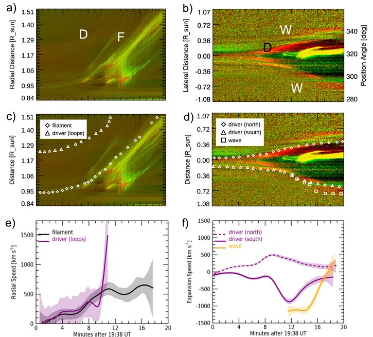
Figure 3. Top: stackplots built from base-difference SDO/AIA two-color composite images (211 Å in red, 171 Å in green), for the 2011 March 7 event. The distance–time plots are measured on a radial slit (panel (a)) and a circular slit at a distance of 1.27 R⊙ (panel (b)). The filament (F), driver (D), and wave (W) are indicated. Middle panels: distance–time plots. (c) Heliocentric distances of driver and filament; (d) distances from the center of the CME for the driver and wave. Bottom: projected speeds derived from the distance–time measurements using the regularization technique in Section 2.3. (e) Radial speed; (f) expansion speed.
Download figure:
Standard image High-resolution imageIn Figure 3(a), we indicate the filament, F, and the high-lying loops, which correspond to the top of the driver D (i.e., the rising CME). We extract the distance values over time (panel (c)) and derive the projected speed profile (panel (e)) for the two features marked as diamonds (filament) and triangles (driver). The right panels in Figure 3 show the evolution of the CME as it crosses a slit parallel to the limb at a distance of 1.27 R⊙. A similar representation was used by, e.g., Cheng et al. (2012) and is useful to visualize the expansion of the CME. In Figure 3(b) we identify the driver D (CME) and the diffuse wave W. We measure the distances of these features from the center (central position angle, CPA) of the CME (diamonds and squares for the northern and southern flanks of the driver, respectively) and the wave (southern flank; squares), as shown in Figure 3(d). From these measurements we can derive the projected expansion speed profiles shown in Figure 3(f). The derived speed and acceleration profiles in both directions, lateral and radial, are obtained via the regularization technique described in Section 2.3. We assume errors of 2% in heights and widths (Veronig et al. 2018).
The radial analysis reveals that the CME front reaches a speed of about 300 km s−1 in the first 10 minutes. The speed then abruptly increases, surpassing 1000 km s−1 within AIA's field of view. The filament, on the other hand, attains a speed of about 500 km s−1.
In the lateral direction, we can distinguish the wave from the CME in one direction only where the projected speeds are larger (bottom right panel), after ∼19:50 UT. We use purple and orange lines to denote the driver and the wave, respectively, following the color convention in Figure 2. We measure a peak projected speed of ∼900 and ∼1100 km s−1 for the driver and the wave (presumably a shock at that point), respectively. The peak in the driver speed occurs a few minutes before the wave top speed. This is the behavior seen in previous analyses and is one of the defining characteristics of EUV waves as fast magnetosonic waves (e.g., Patsourakos & Vourlidas 2012; Downs et al. 2021). The evolution of the lower CME flank in the two channels also indicates shock formation. The lower flank is primarily red, indicating hot 2 MK plasma at the wave front, which, when it separates from the CME, reveals a cooler (green) component.
We note that the sharp change in the radial and lateral kinematics occurs at the same time, at around 19:48 UT. However, these one-dimensional measurements provide only an approximation of the actual 3D kinematics. It is not immediately obvious, for example, why the shock appears only on the south side of the CME. Is the northern flank expanding at a lower rate, or is the wave obscured by a line-of-sight effect? On the other hand, a cut at a given height does not follow the same location along the CME front, since we cannot be sure that the event is expanding self-similarly relative to its expansion center. For these reasons, it is necessary to expand the analysis into three dimensions by taking advantage of our multi-viewpoint observations.
The near-quadrature AIA and EUVI-A views (separation angle of 88°) are favorable for analyzing the 3D evolution of the CME and formation of the wave. We model the 3D shape of both the driver (CME) and the wave using AIA and EUVI-A/B images with a 2.5-minute cadence. A sequence of three snapshots showing the evolution of the CME (top row) and wave (bottom row) in the low corona is shown in Figure 4, with the corresponding 3D models overlaid. The details of the evolution of the parameters derived from these 3D reconstructions are presented in Section 4.

Figure 4. 3D reconstruction of the 2011 March 7 event as seen from STA. Top row: CME (driver). The yellow mesh represents the GCS model. The white crosses and yellow line on the surface indicate the orientation of the main axis of the flux rope. Bottom: wave. The white mesh corresponds to the ellipsoid model. The blue (cyan) and red (orange) line represent the ellipsoid cross sections along the a and b semi-axes, respectively.
Download figure:
Standard image High-resolution image3.2. The 2011 June 7 Event
Figure 5 presents a sequence of four pairs of images (AIA on the top and EUVI-A on the bottom) with the early evolution of the CME and associated wave of the 2011 June 7 CME. The eruption originated in NOAA AR 11226 (S21W64) on the western solar limb as seen from Earth, on the east limb as seen from EUVI-A, and behind the west limb for EUVI-B. The event was visible in the field of view of the EUV instruments from 06:20 to 06:30 UT. A GOES M2.5-class flare began on 2011 June 7 at 06:16 UT and peaked at 06:30 UT. The onset of the CME coincides with the development of the solar flare. Both the Learmonth and Culgoora radio spectrographs report a metric type II burst in association with the flare. Culgoora, however, reports two metric type II bursts 6 in close succession. We suspect that they may be the same burst, but this requires further analysis that is beyond our current scope. We consider here the parameters of the first burst, which is close in time to the one reported by Learmonth. The burst lasted from 06:26 to 06:40 UT and was detected between 140 and 30 MHz, with a derived speed of 850 km s−1. The burst was also detected at lower frequencies (16 MHz to 250 KHz) by both the Wind and STA radio experiments between 06:45 and 18:00 UT, indicating that the shock, or subsequent shocks, lasted into the inner heliosphere. We discuss the radio observations in Section 5.
Figure 5. 2011 June 7 event as seen by AIA (top) and EUVI-A (bottom). The sequence shows different stages in the CME early evolution and wave formation. (a) Rising filament. (b) Early CME (bubble) formation. (c) Lateral expansion of the CME, D, leading to the formation of the wave, W. (d) The separation of the wave (W; orange line) from the driver (D; purple line) is clearly observed. All frames are base-difference images. The yellow dashed lines in panels (a) and (d) indicate the direction for the radial and circular slits used to build the stackplots in Figure 6. An animation of the bottom panels of this figure is available. The animation includes the EUVI-A 195 Å image on the left and the corresponding base-difference image on the right. The animation sequence starts at 06:00:30 UT and ends at 06:38:00 UT. The time lapse between images is 2.5 minutes.
(An animation of this figure is available.)
Download figure:
Video Standard image High-resolution imageFirst, we inspect the sequence of EUV images. A filament is seen to slowly rise from 06:15 to 06:21 UT, as well as the faint overlaying loops. At 06:23 UT, the front of the CME becomes clearer, particularly in the AIA images. Between 06:25 and 06:30 UT, the CME undergoes significant lateral expansion. These stages can be appreciated in the time-slice plots in Figure 6 that show the height evolution along the direction marked by the yellow dashed line in Figure 5(a) and the lateral distance measured parallel to the limb at a fixed height of 1.02 R⊙, respectively. We mark the driver D and filament F in Figure 6(a). From their distance–time measurements (panel (c)) we determine the projected radial speed shown in Figure 6(e) (squares and triangles for driver and filament) using the regularization technique in Section 2.3. In Figure 6(b) we identify the diffuse wave W and the driver D. The distances from the center of the CME are extracted and marked as triangles (driver) and squares (wave) in Figure 6(d) and used to determine the expansion speeds shown in Figure 6(f). For this event, the CME slowly reaches a speed of ∼100 km s−1 as it rises during the first 8 minutes and then increases abruptly to 1000 km s−1 within 4 minutes during the impulsive phase. The expansion speed of the CME, on the other hand, reaches a peak of ∼700 km s−1 during the same phase.
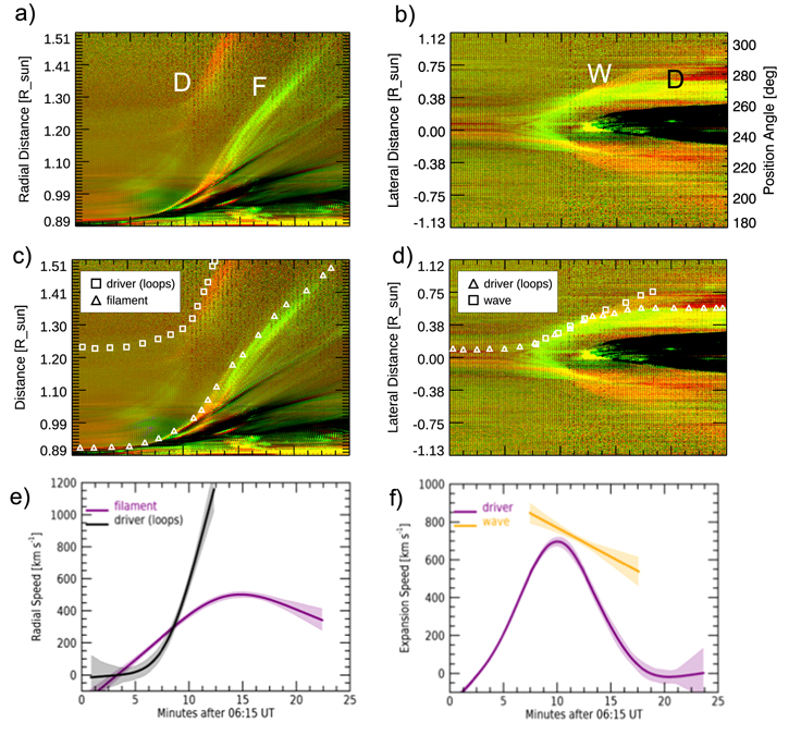
Figure 6. Top: stackplots built from base-difference SDO/AIA two-color composite images (211 Å in red, 171 Å in green), for the 2011 June 7 event. The filament (F), the driver (D), and the wave (W) are indicated. The distance–time plots are measured on a radial slit (panel (a)) and a circular slit at a distance of 1.02 R⊙ (panel (b)). Middle panels: distance–time plots. (c) Heliocentric distances of driver and filament; (d) distances from the center of the CME for the driver and wave. Bottom: projected speeds derived from the distance–time measurements using the regularization technique in Section 2.3. (e) Radial speed; (f) expansion speed.
Download figure:
Standard image High-resolution imageWe next investigate the 3D evolution of both the CME and the wave at heliocentric distances close to the Sun. For this, we take triplets of EUVI and AIA images to fit the GCS and ellipsoid model to the CME and the wave, respectively. Figure 7 shows three snapshots with the reconstruction of the CME and wave overlaid to AIA images. We analyze the evolution of the deprojected heights and widths derived from these reconstructions in the next section.

Figure 7. 3D reconstruction of the CME (yellow grid) and the shock (white grid) in the low corona for the 2011 June 7 event. The white crosses and yellow line on the surface indicate the orientation of the main axis of the flux rope. The blue (cyan) and red (orange) lines represent the ellipsoid cross sections along the a and b semi-axes, respectively. Left: AIA. Right: EUVI-A.
Download figure:
Standard image High-resolution image4. The 3D Kinematic Evolution of the CME and Associated Wave
4.1. Radial Evolution
First, we study the outward/radial propagation of the CME and the wave for both events, as shown in Figure 8. The top panels show in black the time variation of the heliocentric distances to the CME top and center ( and
and  ). The orange symbols and lines represent the heliocentric distances to the wave top and center (
 and
and  ). The symbols mark the values from the 3D reconstruction at each time stamp, along with their respective error bars. Following Kwon et al. (2014), we assume errors in the heights of ±7% for the flux rope and ±8% for the ellipsoid. The solid curves correspond to the fits from the regularization technique described in Section 2 (CME/wave front, solid lines; CME/wave center, dashed lines). The speed and acceleration profiles also from the regularization technique are shown in panels (b) and (c) and panels (d) and (e), respectively. For clarity, we plot the speed and acceleration profiles for the front and the center of the flux rope and the wave separately. The shaded bands represent the corresponding 95% CI intervals.
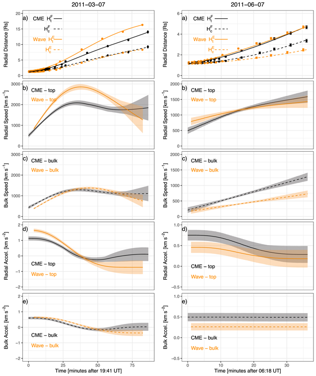
Figure 8. 3D kinematic characterization of the propagation of the CME (black) and the shock wave (orange). (a) Radial distance vs. time. (b) Speed of the top vs. time. (c) Bulk speed vs. time. (d) Acceleration of the top vs. time. (e) Acceleration of the bulk vs. time. The shaded bands represent the error bars for the derived speed and acceleration profiles.
Download figure:
Standard image High-resolution imageWe find that at heliocentric distances below 5 R⊙ the CME and the wave evolve very similarly (top panels of Figure 8) for both events, with the wave front lying close to the top of the CME ( ≃
≃  ). At these low heliocentric distances, the speed of the CME top ranges between about 1500 and 2000 km s−1 (panel (b), black line). We note that when measuring the heights of the top of the CME, the measurements include the contribution of the expansion in the radial direction in addition to the bulk speed (i.e., measured by the motion at the center of the structure). These measurements are still useful and included here because they allow for the comparison with the equivalent projected quantities shown in Section 3. The propagation of the CME, however, is more appropriately characterized by the bulk motion, i.e., the time variation of
  . For this, we find that the peak speed of the CME center (or peak bulk propagation speed) ranges between 1000 and 1200 km s−1 (panel (c)).
Although the impulsive acceleration phase in the CME propagation is not fully captured with the 3D reconstruction (Figure 8(d)), we see that the acceleration of the CME front decreases from ∼1 to ∼0.5 km s−2 within 5 R⊙, in both events. The bulk acceleration, on the other hand, exhibits much less variability with values closer to 0.5 km s−2, indicating that much of the variation in speed of the front comes from the CME expansion rather than propagation (Figure 8(e)).
4.2. Lateral Evolution
Next, we analyze the lateral expansion evolution of the CME and the wave for both events (Figure 9). We consider two main directions for the CME expansion: across and along the main axis of the MFR, i.e., the face-on and edge-on views. The top panels plot the time variation of the CME edge-on ( ) and face-on (
 ) half widths in magenta and blue, respectively. We include in orange the parameters from the ellipsoid model for the wave.
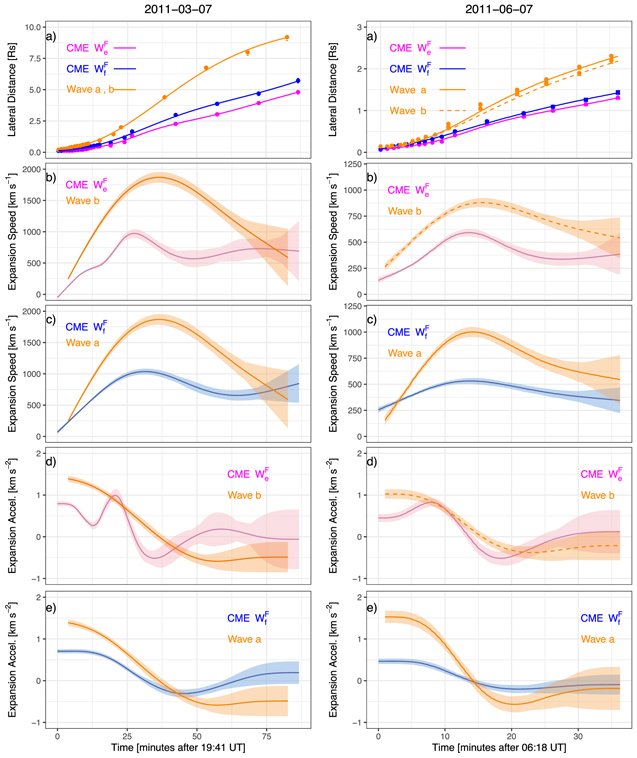
Figure 9. 3D kinematics characterization of the expansion of the CME (blue and magenta) and the shock wave (orange). (a) Distance from the center of the structure vs. time. (b) Expansion speed (across the FR main axis) vs. time. (c) Expansion speed (along the FR main axis) vs. time. (d, e) Expansion acceleration vs. time (across and along the FR main axis). The shaded bands represent the error bars for the derived speed and acceleration profiles.
Download figure:
Standard image High-resolution imageSince the cross section of the GCS model for the CME is circular, there is no difference between the expansion in the radial direction and the lateral direction for the edge-on view, which are parallel and perpendicular to the direction of propagation, respectively. For the wave, however, we can consider the expansion in three directions given by the time variation of the ellipsoid semi-axes. These are the "lateral" expansion in the two directions perpendicular to the outward motion of the CME (given by a and b) and the expansion in the radial direction (given by c). The time variations of the a and b semi-axes are shown in orange.
We plot separately the speed profiles from the distance–time fits via the regularization technique for the edge-on (in panel (b)) and face-on (in panel (c)) half widths of the CME. We then compare them with the equivalent quantities from the ellipsoid model, i.e., the semi-axes b for the edge-on view and a for the face-on view. Similarly, we plot the corresponding acceleration profiles in panels (d) and (e).
We find that in both events the wave expansion speed overtakes the CME expansion speed early in the event evolution, at heliocentric distances below 2 R⊙ as we infer when comparing with Figure 8(a)).
In the March event, the three semi-axes are similar to the edge-on and face-on half widths of the CME until about 20:07 UT (Figure 9(a)). Both CME and wave are accelerating as seen in panels (b) and (c). Between 20:09 and 20:24 UT, however, the wave continues to accelerate in the lateral directions while the CME decelerates. As a result, the wave expands rapidly, reaching a peak speed of 2000 km s−1 at 20:24 UT while the CME lateral growth slows down, having achieved a top speed of 1000 km s−1 between 20:10 and 20:11 UT. We note three interesting behaviors in the left panels: (i) the divergence in the CME/wave speeds precedes by about 2−3 minutes the separation of the wave and CME fronts, (ii) the speed and acceleration behavior of the wave follows closely the behavior of the face-on width of the CME, and (iii) the CME face- and edge-on speeds and accelerations are similar. Observations (i) and (ii) are the expected behaviors for a wave−driver pair (Lulić et al. 2013). Namely, the CME lateral expansion leads to compression of the ambient plasma and the creation of a wave front that stays close to the CME flank until the driver begins to decelerate (after about 19:55 UT). The wave (most likely a shock by that time) escapes with enough energy to reach 2000 km s−1 and begins to decelerate after 20:24 UT. This is also the time when the CME widths reach a constant, and similar, speed of about 700 km s−1.
The June event exhibits similar characteristics, albeit at lower levels, reflecting the lower impulsiveness of this event. In this case, the wave evolution seems to track the CME edge-on width slightly closer than the CME face-on width, but the behaviors are not significantly different than for the March event. The wave begins to separate from the CME flank from 06:30 UT onward (panel (a)). This is the same time that the CME face-on width begins to decelerate. By 06:32 UT, both CME widths are decelerating. The CME expansion (for both the face-on and edge-on widths) reaches ∼600 km s−1, with the wave expansion speeds almost twice as much.
5. Discussion
With the radial (Figure 8) and lateral (Figure 9) kinematic profiles for the CME and its associated wave/shock in hand, we can now proceed toward the core objective of this work. Namely, we can decouple the bulk propagation from the expansion in the different directions (radial and lateral) in order to examine whether a hyper-inflation phase does indeed occur during the early evolution of the CMEs. For that, we inspect the time profile of the aspect ratio of the CME. The aspect ratio is defined as the ratio of the CME center height to the radial/lateral width ( /
/ ).
).
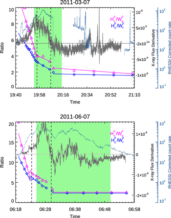
The two aspect ratios are plotted in Figure 10: radial (edge-on; magenta curve) and lateral (face-on; blue curve) for both events. For comparison, we include the time derivative of the soft X-ray (SXR) flux from GOES (black curve), which is generally used as a proxy of the energy release (Dennis & Zarro 1993). In addition, the hard X-ray emission measured by RHESSI (Lin et al. 2002) in the 12–25 keV range for both events is also shown in blue (rightmost axis). The area in green indicates the duration of the metric type II radio burst associated with each event (Table 1).
Figure 10. Variation of the CME apex height to width ratio vs. time. The derivative of the SXR flux is shown in gray. The RHESSI light curve in the 12–25 keV energy band is shown as blue circles. The area in green represents the duration of the metric type II radio burst associated with the events (reported by Sagamore Hill and Learmonth stations for the March and June events, respectively).
Download figure:
Standard image High-resolution image
The aspect ratio evolution shows many similarities in both events. The slow rise phase of the CME is marked by a strong expansion manifested by the sharp drop in both the lateral and radial aspect ratios. The radial expansion starts from a higher aspect ratio than the lateral aspect ratio. The radial dimension of the bubble may be underestimated, however, at the very early stages of the event, when the expanding EUV bubble is small and its boundaries are difficult to discern against the surrounding loop background. Since the CME MFR reconstruction is inherently cylindrical in geometry, it may underestimate the radial compared to the lateral dimensions (see also Figure 1).
Unfortunately, there is no observational way to constrain the size of the CME at those early instances owing to its small size and the confusion by intervening structures in the core of the active region.
Overall, both aspect ratios decrease drastically within a short time interval (14 and 3 minutes for the March and June events, respectively), which coincides with the energy injection phase of the flare, as inferred from the X-ray flux derivative. Another indication is given by the HXR profiles, which also show a peak during the overexpansion phase, following closely the CME evolution as suggested by Temmer et al. (2008, 2010).
Looking into the profiles in more detail, we can identify three stages in the aspect ratio evolution, indicated by the vertical dashed lines in Figure 10: (i) during the first stage, the CME experiences a rapid overexpansion both laterally and radially; (ii) the expansion slows down in the second phase, but the event continues to overexpand until (iii) the third stage, where the CME aspect ratio becomes constant (at a ratio of about 2, for both events), indicating a self-similar expansion. Interestingly, the third stage coincides with the end of the flare energy release phase (SXR derivative reaches zero) for both events.
We quantify the evolution of the aspect ratio by fitting linear curves to each of the three stages (Table 2). For the 2011 March 7 event, the radial ratio ( /
/ ) decreases at a rate of 0.53 minute−1 between 19:41 and 19:54 UT, slowing down to 0.07 minute−1 from 19:55 and 20:09 UT. The rate of change of the lateral aspect ratio reduces from 0.25 to 0.09 minute−1 in the same time intervals, respectively. The June event exhibits a more drastic hyper-inflation phase in its radial aspect ratio, but the slope may be overestimated as we discussed earlier. Within just 3 minutes (06:18–06:21 UT), the
  /
/ ratio decreases at a rate of 2.88 minute−1, slowing down to a rate of 0.41 minute−1 between 06:22 and 06:28 UT. The rate of change of the lateral aspect ratio (
 /
/ ) changes from 1.49 to 0.51 minute−1 for the same time intervals.
Table 2. Summary of the Three-stage Temporal Evolution of the CME Radial and Lateral Aspect Ratio for the Two Analyzed Events
| 2011 Mar 7 | 2011 Jun 7 | |||||
|---|---|---|---|---|---|---|
| Stage | Time | Rate of Change | Time | Rate of Change | ||
| (UT) | Radial | Lateral | (UT) | Radial | Lateral | |
| (minute−1) | (minute−1) | (minute−1) | (minute−1) | |||
| Hyper-inflation | 19:41–19:54 | −0.53 | −0.25 | 06:18–06:21 | −2.88 | −1.49 |
| Slow expansion | 19:55–20:09 | −0.07 | −0.09 | 06:22–06:28 | −0.41 | −0.51 |
| Self-similar | 20:09–21:07 | −0.01 | −3 × 10⁻³ | 06:29–06:54 | −7 × 10⁻⁵ | −4 × 10⁻⁵ |
Note. The gradients are results of linear fits to the aspect ratio measurements shown in Figure 10.
Download table as: ASCIITypeset image
Another noteworthy observation is that the metric type II radio burst starts at, or very closely after, the end of the first stage, i.e., the hyper-inflation phase (green area in Figure 10 and Table 1). An inspection of the expansion speed profiles for the CME and the wave in Figure 9 reveals that the radio emission starts when the wave expansion speed exceeds the CME expansion speed. Taking into account the uncertainties in the speed measurements, we find that the June event wave separates from the CME at 06:22 ± 1 minute along the radial and at 06:24 ± 1 minute along the lateral direction while the metric type II starts at 06:25-26 UT (Table 1). For the March event, the wave separates at 19:51 ± 1 minute along the radial and at 19:53 ± 1 minute along the lateral dimensions while the type II starts at 19:54. In other words, the start time of the type II is in excellent agreement with the time of wave−CME separation along the lateral direction and with the end of the hyper-inflation stage, for both events. Previous works (e.g., Kouloumvakos et al. 2013) have reported on the close association between metric type II radio bursts and EUV waves but have generally failed to resolve the long-standing ambiguity of whether the emission arises from the flanks of the CME (e.g., Gary et al. 1984; Patsourakos et al. 2010a; Demoulin et al. 2012) or the CME nose (as suggested by Kozarev et al. 2011; Ma et al. 2011). Our analysis provides strong support to the CME flank scenario, demonstrating that the radio emission is observed at, or near, the peak of the CME lateral hyper-inflation phase when the EUV wave becomes a shock (as indicated by the appearance of the metric type II emission). Therefore, the lateral hyper-inflation phase of the CME is driving the wave/shock formation as suggested by Patsourakos & Vourlidas (2012) and supported by simulations (see, e.g., Vršnak et al. 2016; Krause et al. 2018; Downs et al. 2021). After its separation from the CME, the expansion speed of the wave reaches a peak value that is twice that of the expansion speed, and this has been interpreted as an indication of a 3D piston mechanism from simulations (Lulić et al. 2013; Vršnak et al. 2016) and EUV observations (Veronig et al.2018).
Although detailed SEP analysis is beyond the current scope, we should briefly comment on the SEP properties of these two events. Both are associated with >25 MeV protons detected at Earth, but only the March event is associated with SEPs detections at STA and STB (Richardson et al. 2014). In a rare coincidence, the angular separations between the three locations (STA, STB, Earth) and the flare site are identical in both events. Assuming, therefore, that the transport effects are similar in these two periods (and ignoring the interplanetary conditions for the sake of this simple comparison), the increased 25 MeV intensity levels in STB (almost equal to the Earth-recorded intensities at 0.5 MeV s cm2 sr−1) must be due to a more efficient shock acceleration in the March event compared to the June event. Indeed, Figures 9–10 show that the CME and wave speeds were lower in the June event, indicating a weaker shock. The likely reason for the weaker shock may be the shorter hyper-inflation stage. It seems to terminate "prematurely" ∼3 minutes before the peak of the SXR derivative compared to the March aspect ratio profiles. While further analysis is needed to establish the dependence of the hyper-inflation phase on SEP production, these initial indications of a connection are nevertheless intriguing.
As noted by Patsourakos & Vourlidas (2012), the hyper-inflation stage could be simply driven by the magnetic pressure within the MFR as it tries to equilibrate with its ambient fields. In this case, though, we would expect the rapid expansion to occur as soon as the EUV bubble clears the active region fields and encounters the lower magnetic fields in the surrounding quiet-Sun regions. This does not seem to be the case for either of the two case studies here. Patsourakos & Vourlidas (2012) also suggested ideal and nonideal processes as potential drivers for the hyper-inflation phase. The "reverse pinch effect" (Kliem et al. 2014) could be an ideal process candidate. As the MFR begins to expand, its internal current is reduced, leading to an expansion of the flux surfaces around the MFR, which would register in the images as rapid expansion of the EUV bubble. Such an effect could possibly account for the rapid decrease in the radial aspect ratio, as the expansion of the surrounding flux surfaces should manifest itself primarily along the radial direction in the images. Furthermore, indications of abrupt changes in the EUV bubble were noted by Vourlidas et al.(2012).
However, the close relation between the energy release (via the SXR derivative and the HXR profile) and the aspect ratio decrease seen in Figure 10 points strongly to a nonideal process such as the addition, via reconnection, of poloidal flux in the erupting MFR (see Veronig et al. 2018 for a detailed analysis of a very similarly behaved event). In fact, such a process naturally explains both the lateral expansion direction (since the poloidal flux leads to the increase of the MFR major radius) and speeds (1000–1500 km s−1), which are compatible with expected reconnection rates at CME current sheets (e.g., Lin et al. 2015, and references therein). It straightforwardly connects the MFR (lateral) growth to flare ribbon expansion and provides strong support to analyses of CME and flare energetics (e.g., Zhu et al. 2020).
It is unsurprising that the hyper-inflation phase has escaped wider recognition in CME studies despite the decade since its discovery. The phase occurs within a very short interval of a few minutes, which requires high-cadence EUV observations, from the proper vantage point (to detect the bubble boundaries), to capture the formation of the EUV bubble and measure its expansion. The 5-minute cadence of our dual-viewpoint reconstructions is barely sufficient to resolve the 3D evolution and explains the difficulty in obtaining large event samples. The currently available high-cadence AIA data do not provide enough constraints on their own, although they could be used in certain cases, under some assumptions about the overall shape of the bubble. In the near term, small angular separation observations from EUVI-A, which is approaching Earth, and from Solar Orbiter may offer additional insights.
In summary, the hyper-inflation phase has broad implications for solar eruption research. In fact, we argue that this stage should be considered as the "missing link" in the connection of CMEs to flares, to shocks, and to SEPs. It represents the creation of the actual ejected MFR (although a preexisting smaller MFR is not excluded by our analysis) that comprises the CME structure images in the coronagraph heights. The process of the MFR creation (the injection of poloidal flux) drives both the EUV waves and metric type II emission. The estimated speeds during the hyper-inflation phase are sufficiently high to generate shocks and to accelerate particles concurrently with the impulsive phase of the SXR flare, thus providing a unified scenario for the origins of SEPs, as shock-accelerated particles. However, further analyses on this topic are needed.
6. Conclusions
As mentioned in the Introduction, the lateral overexpansion of CMEs in the low corona has been suspected and reported in previous studies, based either on single-viewpoint high-cadence EUV data (see, e.g., Patsourakos et al. 2010a, 2010b; Cheng et al. 2012; Veronig et al. 2018) or on 3D reconstructions (Cremades et al. 2020; Majumdar et al. 2020). While Patsourakos & Vourlidas (2012) recognized the implications of a strong low coronal expansion phase for understanding shock development, there was a dearth of reliable 3D information in that coronal region to establish the existence and properties of this hyper-inflation phase. The analysis presented here aimed at filling this gap by verifying that such a phase does indeed occur during the very early development of CMEs.
We analyzed multi-viewpoint EUV observations of the formation and early evolution of two bubble-like CMEs and their associated waves. Using forward modeling, we characterized the 3D kinematics of the nascent CME and the wave for the 2011 March 7 and 2011 June 7 CMEs. Both events were accompanied by metric type II radio emission and SEPs. From the comparison of the propagation and expansion profiles we determined the radial and lateral expansion speeds, as well as the bulk propagation speeds. The speed analysis revealed that the metric type II emission (which is a reliable coronal shock proxy) starts, for both events, at the end of the initial rapid lateral growth of the CME (hyper-inflation phase). At that moment, the EUV separates from its CME driver and continues to accelerate for a few minutes, driving presumably the shock related to the radio emission.
More importantly, we were able to construct both radial and lateral aspect ratios of the CMEs by dividing the CME center height with the radial/lateral sizes, as estimated from the GCS fits. The temporal evolution of the aspect ratio revealed intriguing behaviors and connections to the energy release rates, estimated via the SXR temporal derivative of the accompanying flare (Figure 10), as follows:
- 1.The CME expansion undergoes three distinct stages: (1) a hyper-inflation stage where the lateral (and, to a lesser degree, radial) size of the CME increases by a factor of 2–3 within 10 minutes, or less; (2) a slower expansion stage that lasts a few minutes; and finally (3) a self-similar expansion where the ratio of CME center to its flanks remains constant.
- 2.The expansion stages (stages 1 and 2) follow very closely the SXR time derivative. The expansion stops, for both events, when the flare energy release also stops.
- 3.The hyper-inflation is stronger along the lateral direction and is responsible for the formation of the EUV wave and subsequent shock and radio emission.
- 4.The difference in the SEP properties of the two events (identical observer−source configurations, but only the March event is associated with a widespread SEP event) seems to be due to the shorter hyper-inflation stage for the June event. Further studies along that direction are needed.
- 5.The end of the hyper-inflation phase coincides with the start of the metric type II radio burst, which indicates the creation of a coronal shock. In both CMEs, the hyper-inflation drives the higher speed at the CME flanks. We thus conclude that the radio emission arises at the (shocked) flanks of the erupting CME.
Our analysis leads us to the following overall conclusion. The hyper-inflation phase likely represents the formation stage of the magnetic structure that is eventually ejected into the corona, as the white-light CME. It appears to be driven by the injection of poloidal flux into the ejecting magnetic structure, which leads to the (primarily) lateral growth of the MFR. The rapid growth results in the creation of EUV waves and eventually shocks at the CME flanks. The shocks are detected as metric type II radio bursts. In other words, the hyper-inflation stage in the early CME evolution may be the "missing" link between CMEs, flares, and coronal shocks.
L.A.B., A.V., and G.S. are supported by LWS grant 80NSSC19K0069. L.A.B. also acknowledges the support from the NASA program NNH17ZDA001N-LWS (award Nos. 80NSSC19K1235 and 80NSSC20K0286). R.-Y.K. acknowledges support from the National Research Foundation of Korea (NRF-2019R1F1A1062079) grant funded by the Korea government (MSIT; project No. 2019-2-850-09). We also would like to thank the referee for their careful reading of the manuscript and useful suggestions and comments.
Footnotes
- 5
- 6