


Abstract
The MAMMOTH–Grism slitless spectroscopic survey is a Hubble Space Telescope (HST) cycle 28 medium program, which is obtaining 45 orbits of WFC3/IR grism spectroscopy in the density peak regions of three massive galaxy protoclusters at z = 2–3 discovered using the MAMMOTH technique. We introduce this survey by presenting the first measurement of the mass–metallicity relation (MZR) at high redshift in overdense environments via grism spectroscopy. From the completed MAMMOTH–Grism observations in the field of the BOSS1244 protocluster at z = 2.24 ± 0.02, we secure a sample of 36 protocluster member galaxies at z ≈ 2.24, showing strong nebular emission lines ([O III], Hβ, and [O II]) in their G141 spectra. Using the multi-wavelength broadband deep imaging from HST and ground-based telescopes, we measure their stellar masses in the range of [109, 1010.4] M⊙, instantaneous star formation rates (SFR) from 10 to 240 M⊙ yr−1, and global gas-phase metallicities ![$[\tfrac{1}{3},1]$](https://content.cld.iop.org/journals/0004-637X/926/1/70/revision1/apjac3974ieqn1.gif) of solar. Compared with similarly selected field-galaxy samples at the same redshift, our galaxies show, on average, increased SFRs by ∼0.06 dex and ∼0.18 dex at ∼1010.1M⊙ and ∼109.8M⊙, respectively. Using the stacked spectra of our sample galaxies, we derive the MZR in the BOSS1244 protocluster core as
of solar. Compared with similarly selected field-galaxy samples at the same redshift, our galaxies show, on average, increased SFRs by ∼0.06 dex and ∼0.18 dex at ∼1010.1M⊙ and ∼109.8M⊙, respectively. Using the stacked spectra of our sample galaxies, we derive the MZR in the BOSS1244 protocluster core as  ×
×  , showing a significantly shallower slope than that in the field. This shallow MZR slope is likely caused by the combined effects of efficient recycling of feedback-driven winds and cold-mode gas accretion in protocluster environments. The former effect helps low-mass galaxies residing in overdensities retain their metal production, whereas the latter effect dilutes the metal content of high-mass galaxies, making them more metal-poor than their coeval field counterparts.
Export citation and abstract BibTeX RIS

Original content from this work may be used under the terms of the Creative Commons Attribution 4.0 licence. Any further distribution of this work must maintain attribution to the author(s) and the title of the work, journal citation and DOI.
1. Introduction
Mapping galaxy properties in different environments across cosmic time is essential to forming a complete picture of galaxy formation and evolution. Galaxy protoclusters at z = 2–3 provide a direct probe of the rapid assembly of large-scale structures at cosmic noon, making them ideal laboratories to test the environmental dependence of galaxy mass assembly and chemical enrichment at the peak of cosmic star formation (e.g., Overzier 2016; Shimakawa et al. 2018). The relative abundance of oxygen compared to hydrogen in the interstellar medium—gas-phase metallicity (hereafter referred to as metallicity for simplicity)—provides a crucial diagnostic of the past history of star formation and complex gas movements driven by galactic feedback and tidal interactions (Lilly et al. 2013; Maiolino & Mannucci 2019). Therefore, measuring the metallicity of galaxies undergoing active star formation in the cores of protoclusters at cosmic noon can probe the effects of galactic feedback versus environment in shaping galaxy chemical evolution (Oppenheimer & Davé 2008; Kulas et al. 2013; Ma et al. 2016).
It is well established that metallicity correlates strongly with galaxy stellar mass (i.e., the mass–metallicity relation: MZR) in both the local and distant universe (Tremonti et al. 2004; Erb et al. 2006; Maiolino et al. 2008; Andrews & Martini 2013; Henry et al. 2021; Sanders et al. 2021). There is also a growing consensus about the role that environment plays in galaxy metal enrichment at z ∼ 0: galaxies situated in overdensities are observed to be more metal enriched than coeval field galaxies of the same mass (Cooper et al. 2008; Ellison et al. 2009). However, at cosmic noon, the situation is highly uncertain, with little or conflicting evidence of the existence of any environmental effects (Kacprzak et al. 2015; Shimakawa et al. 2015; Valentino et al. 2015), primarily due to small number statistics.
In this paper, we present the first attempt to measure the high-z MZR in overdense environments using space-based slitless spectroscopy from a sample of 36 protocluster member galaxies showing prominent nebular emission lines. The high throughput of the Wide-Field Camera 3 (WFC3) grism channels on board the Hubble Space Telescope (HST) and the low infrared (IR) sky background in space enable us to probe the metal enrichment in protocluster member galaxies down to a very low stellar mass of M* ∼ 109 M⊙ at z = 2.24. In addition, we measure a pure emission-line-selected sample unbiased by photometric preselection due to the slitless nature of WFC3's grism spectroscopy. Throughout this work, we adopt the AB magnitude system and the standard concordance cosmology (Ωm = 0.3, ΩΛ = 0.7, H0 = 70 kms−1Mpc−1). The metallic lines are denoted in the following manner, if presented without wavelength: [O III]λ5008: = [O III], [O II]λ λ3727, 3730: = [O II], [Ne III] 3869: =[Ne III], [N II] λ6585: = [N II].
2. Grism Observation of the MAMMOTH Protocluster BOSS1244
The BOSS1244 protocluster (z = 2.24 ± 0.02) was discovered via the MAMMOTH (MApping the Most Massive Overdensity Through Hydrogen) technique, which identifies the extreme tail of the matter-density distribution at high redshifts using coherently strong intergalactic Lyα absorption in background quasar spectra (Cai et al. 2016, 2017a, 2017b). This identification is drawn from the entire SDSS-III quasar spectroscopic sample (Alam et al. 2015) over a sky coverage of 10,000 deg2, suggesting that BOSS1244 is one of the most massive galaxy protoclusters at cosmic noon. Deep CFHT broad+narrowband imaging has revealed pronounced overdensities of Hα emitters (HAEs), most of which are spectroscopically confirmed by LBT/MMT IR spectroscopy (Shi et al. 2021; Zheng et al. 2021, also see the left panel of Figure 1). Within a (15 cMpc)3 volume, the density peak region of BOSS1244 in the southwest has a galaxy overdensity of δgal = 22.9 ± 4.9, where the galaxy overdensity is defined as δgal = Σcluster/Σfield − 1 with Σcluster/field corresponding to the HAE number counts per arcmin2 in the protocluster/blank fields at the protocluster redshift. The derived δgal of BOSS1244 is a factor of ≥ 2 larger than that measured in other protoclusters at similar redshifts, e.g., SSA22 at z = 3.1, which is estimated to have δgal = 9.51 ± 1.99 within a (16 cMpc)3 volume (Topping et al. 2018). This high δgal of BOSS1244 corresponds to a present-day total enclosed mass of (1.6 ± 0.2) × 1015 M⊙. BOSS1244 will likely evolve into a galaxy cluster more massive than Coma at z ∼ 0; therefore, it is an excellent example of the most extremely overdense environments at z ≥ 2.

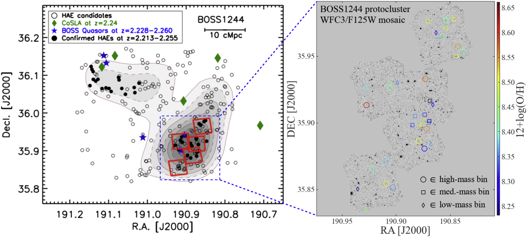
Figure 1. The BOSS1244 protocluster center field targeted by the MAMMOTH–Grism program and presented in this work. Left: the density map for the massive protocluster BOSS1244 at z = 2.24 ± 0.02. The density contours (shown in brown and filled in gray) for Hα emitters (HAEs) are shown in steps of 0.2 arcmin−2, with the inner density peak reaching ∼2 arcmin−2. The green diamonds are the groups of Lyα absorption systems from background high-z BOSS quasars, and the blue stars are the quasars at the protocluster redshift. The black circles are the HAE candidates selected through CFHT broad+narrowband imaging and the black solid points are spectroscopically confirmed by ground-based IR spectroscopy (Shi et al. 2021). It is expected to have a present-day total enclosed mass of ≳ 1.6 × 10¹⁵ M⊙, likely evolving into a local Coma-like supercluster. The density peak regions of the BOSS1244 protocluster in the southwest are targeted by MAMMOTH–Grism, with 5 pointings of WFC3/G141+F125W, each pointing at 3 orbit depth, highlighted by the red squares. Right: A zoom-in view of the BOSS1244 density peak regions (marked by blue dashed box in the left panel) on the F125W image mosaics acquired by MAMMOTH–Grism. This F125W imaging is a coaddition of the pre-imaging component (with an average depth of 1800 sec) to the G141 grism exposures. Using the deep G141 grism spectroscopy, we secure a total of 36 star-forming protocluster member galaxies at z ∼ 2.24, showing extreme emission lines of [O III], Hβ, and [O II]. They are color-coded by their inferred metallicity assuming the (Bian et al. 2018, B18) strong line calibrations as described in Section 3.5, and represented by three sets of symbols corresponding to the three mass bins, chosen for the stacking analysis (see Section 3.4).
Download figure:
Standard image High-resolution imageWe are conducting the MAMMOTH–Grism slitless spectroscopic survey to obtain followup slitless spectroscopy of three MAMMOTH protoclusters (with BOSS1244 being one of them). MAMMOTH–Grism is an HST cycle-28 medium program (GO-16276, P.I.: X. Wang), awarded 45 primary orbits to acquire deep WFC3/G141-F125W observations in the centers of three of the most massive galaxy protoclusters at z = 2–3. The observations in the BOSS1244 field were completed in 2021 February, with a total of 5 different pointings, each at 3 orbit depth. To mitigate the spectral collision effect of crowded fields, for each pointing, we design a set of 3 individual visits of 1 orbit G141 grism + F125W direct imaging exposures, with an incremental orient offset of 10–15 degrees among the three visits. This results in ∼6 ks of G141 spectroscopy (covering 1.1–1.7 μm) and ∼1.8 ks of F125W imaging, useful for the astrometric alignment and wavelength calibration of the paired grism exposure. In total, MAMMOTH–Grism acquired 30 ks of G141 and 9 ks of F125W exposures in the field of the BOSS1244 protocluster (see the right panel of Figure 1).
3. Measurements
3.1. Grism Redshift and Emission-line Flux
We utilize the Grizli 8 software (Brammer & Matharu 2021) to reduce the WFC3/G141 data. Briefly, Grizli analyzes the paired direct imaging and grism exposures in five steps: 1) pre-processing of the raw WFC3 exposures (e.g., relative/absolute astrometric alignment, flat-fielding, variable sky background subtraction due to helium air glow, etc.), 2) forward-modeling full-FoV grism exposures at the visit level, 3) redshift fitting via spectral template synthesis, 4) full-FoV grism model refinement, and 5) 1D/2D grism spectrum and emission-line map extraction for individual extended objects.
Our deep grism spectroscopy allows robust redshift measurements following the method detailed in Appendix A of Wang et al. (2019). In brief, we fit linear combinations of spectral templates to the observed optimally extracted 1D grism spectra of sources to search for their best-fit grism redshifts. The source's grism redshift fit is considered to be secure only if all the following goodness-of-fit criteria are met (i.e., the reduced χ2, the width of the redshift posterior, and the Bayesian information criterion):  . As a result, we obtain a sample of 284 galaxies in the redshift range of z ∈ [0.15, 4], whose grism redshifts are deemed secure according to the above joint selection criteria. Their redshift histogram is shown in Figure 2. There are in total 55 galaxies (shown in orange in Figure 2) with secure grism redshifts of z ∈ [2.15, 2.35], corresponding to the likely member galaxies of the BOSS1244 protocluster spectroscopically confirmed at z ∼ 2.24 (Shi et al. 2021, marked by the vertical red dotted line in Figure 2). Note that the spectroscopic confirmation of BOSS1244's redshift was performed using the ground-based MMT/MMIRS and LBT/LUCI K-band multi-object spectroscopy of HAE candiates, with high-wavelength resolution of R ∼ 1200–1900 (Shi et al. 2021). Albeit with lower wavelength resolution (R ∼ 130), our grism analysis independently confirms the extremely overdense nature of the BOSS1244 center field, as shown in Figure 2.

Figure 2. Redshift histograms of galaxies along the line of sight to the BOSS1244 protocluster density peak regions probed by MAMMOTH–Grism. Here we only include galaxies whose grism redshifts (zgrism) are considered to be secure according to the joint criteria mentioned in Section 3.1. The vertical red dotted line denotes the measured spectroscopic redshift of BOSS1244 as zspec = 2.24 ± 0.02 reported by Shi et al. (2021). Note that zspec was measured with ground-based multi-object spectroscopic instruments with higher wavelength resolution than that of WFC3/G141, so zspec is usually deemed more precise than zgrism (see, e.g., Matharu et al. 2019). The orange histogram marks the redshift range of z ∈ [2.15, 2.35] where the protocluster member galaxies are selected. The entire line-of-sight structure is mapped out by our deep WFC3/G141 slitless spectroscopy, which independently confirms the extremely overdense nature of the BOSS1244 center field.
Download figure:
Standard image High-resolution imageWhen deriving the best-fit grism redshifts of our targets of interest, we also fit for their intrinsic nebular emission lines with 1D Gaussian profiles centered at the corresponding wavelengths, and thus obtain their line fluxes. We thereby obtain flux measurements of multiple emission lines ([O II], [Ne III] 9 , Hδ, Hγ, Hβ, [O III]) in the sample of secure protocluster member galaxies. To secure accurate metallicity estimates, we select sources with strong detections of [O III] and [O II] (both with SNR ≳ 3). This results in a final sample of 39 protocluster member galaxies showing prominent nebular emission features for the subsequent analyses. Their measured line fluxes are presented in Table 1.
3.2. Stellar Mass and Star Formation Rate
There has been a wealth of multi-wavelength deep imaging data in the field of BOSS1244. In addition to the F125W imaging acquired by MAMMOTH–Grism, we take advantage of the archival HST/WFC3 F160W imaging at 1 orbit depth (obtained by GO-15266, P.I.: Z. Cai). Both the F125W and F160W imaging data have been reduced using the AstroDrizzle software, drizzled onto a common pixel grid with 0 06 pixel scale and pixfrac
=
0.8, astrometrically aligned to the GAIA DR2 astrometry frame (Brown et al. 2018).
06 pixel scale and pixfrac
=
0.8, astrometrically aligned to the GAIA DR2 astrometry frame (Brown et al. 2018).
We also utilize the existing ground-based imaging data in the field, which includes LBT/LBC Uspec imaging (exposure time: 4.65 hr, 5σ limiting magnitude: 26.67 mag for a slightly extended source with a 2'' diameter), LBT/LBC z-SLOAN imaging (exposure time: 3.92 hr, 5σ limiting magnitude: 25.12 mag for an extended source with a 2'' diameter), and CFHT Ks imaging (exposure time: 7.50 hr, 5σ limiting magnitude: 23.29 mag for an extended source with a 2'' diameter). The typical seeing condition during the data acquisition of these ground-based data is 06–09 (D.D. Shi 2021, in preparation).
We run SExtractor in dual mode to perform aperture photometry of the HST imaging data, with the stacked F125W and F160W mosaics as the detection image to increase the depth. The total magnitudes in F125W and F160W are then measured from the corresponding isophotal fluxes with proper aperture correction. To account for the large difference between the HST and ground-based imaging resolutions, we adopt the T-PHOT software (Merlin et al. 2016) that does template fitting of low-resolution images using a priori knowledge of object position/morphology from high-resolution images. By minimizing the low-resolution image residuals after removing a combination of models built from high-resolution templates, we obtain accurate photometric measurements from the ground-based imaging data compatible with the isophotal fluxes measured from HST images (Laidler et al. 2007). As a consequence, we obtain broadband photometry over a wide wavelength range of [1000, 7000] Å in the rest frame for the 39 selected protocluster member galaxies at z ∈ [2.15, 2.35].
To estimate the stellar masses (M*) of our sample galaxies, we use the BAGPIPES software (Carnall et al. 2018) to fit the BC03 (Bruzual & Charlot 2003) models of spectral energy distributions (SEDs) to the photometric measurements derived above. We assume the Chabrier (2003) initial mass function, a metallicity range of Z/Z⊙ ∈ (0, 2.5), the Calzetti et al. (2000) extinction law with Av in the range of (0, 3) and an exponentially declining star formation history with τ in the range of (0.01, 10) Gyr during the SED fitting. The redshifts of our galaxies are fixed to their best-fit grism values, with a conservative uncertainty of Δz/(1 + z) ≈ 0.003, following Momcheva et al. (2016). Note that we also obtain the actual measurements of Δz/(1 + z) for our galaxies, where Δz is given by the half width between the 16th and 84th percentiles of the redshift posteriors calculated by Grizli. The median, minimum, and maximum values of Δz/(1 + z) for our sample is 5.5 × 10⁻⁴, 1.3 × 10⁻⁴, 2.0 × 10⁻³, respectively. This is in fair agreement with the finding by Momcheva et al. (2016). Our smaller redshift errors are primarily driven by the fact that our sample sits on a sweet spot of z ∼ 2.2–2.3 where G141 is particularly efficient and accurate at measuring redshifts of prominent line emitters whose multiple emission features (i.e.,[O III], Hβ, [O II]) are covered simultaneously by this grism element. For simplicity, we adopt Δz/(1 + z) = 3 × 10⁻³ throughout the entire sample as a conservative uncertainty on galaxy redshift in SED fitting. The nebular emission component is also added into the SED during the fit, since our galaxies are exclusively strong line emitters by selection.
We use the Balmer line luminosities to estimate the instantaneous star formation rate (SFR) of our sample galaxies. This approach provides a valuable proxy of the ongoing star formation on a timescale of ∼10 Myr, highly relevant for galaxies displaying strong nebular emission lines. From our forward-modeling Bayesian method described in Section 3.5, we can put stringent constraints on the de-reddened Hβ flux. Assuming the Kennicutt (1998) calibration and the Balmer decrement ratio of Hα/Hβ = 2.86 from the case B recombination for typical H II regions, we calculate

suitable for the Chabrier (2003) initial mass function. The derived M* and SFR values for our entire galaxy sample are given in Table 1.
In the left panel of Figure 3, we show the loci of our protocluster member galaxies in the SFR–M* diagram. The individual galaxies are represented by gray diamonds, whereas the median values within the three mass bins (defined in Section 3.4) are shown by red diamonds. To facilitate a comparison with field galaxies in the similar M* range at the same z, we rely on the galaxy sample at z ∼ 2.3 from the MOSDEF survey (Kriek et al. 2015; Shapley et al. 2015) because the MOSDEF galaxies are also emission-line-selected with SFRs estimated from Balmer line fluxes. The best-fit SFR–M* relation for the z ∼ 2.3 MOSDEF galaxies is shown as the blue dashed line in the left panel of Figure 3, with the cyan shaded band representing its 1σ uncertainty. Sanders et al. (2021) show that the MOSDEF sample is representative of galaxies on the star-forming main sequence (SFMS) at z ∼ 2.3 in the stellar mass range of 109–1010.75
M*. The median values from our protocluster galaxy sample show enhanced SFRs by 0.06, 0.18, and 0.37 dex as compared to the MOSDEF SFR–M* relation. To make a fair comparison, we also need to account for the different line flux limits from the two surveys. The 3σ limiting line flux for our 3 orbit G141 MAMMOTH–Grism exposures is 1.7 × 10⁻¹⁷ ergs−1cm−2 (also see Atek et al. 2010; Momcheva et al. 2016). This is 0.28 dex higher than the MOSDEF detection limit, which is 1.5 × 10⁻¹⁷ ergs−1cm−2 at 5σ within a 2 hr observation reported by Kriek et al. (2015). Our Hβ line flux detection threshold thus translates into an SFR limit of 9.2 M⊙ yr−1, represented by the dotted–dashed line in Figure 3. Comparing our SFR threshold with the 1σ spread of the MOSDEF galaxies, we see that our detection threshold allows complete sampling of the SFMS at z ∼ 2.24 down to M* ∼ 109.7
M⊙. We therefore argue that the SFR increases detected in our intermediate- and high-mass bins are robust and primarily stem from the environmental effect. We also tentatively observe that the star formation enhancement induced by overdense environments is more prominent for lower-mass galaxies: ΔSFR ≈ +0.18 dex in our galaxies with  and ΔSFR ≈ +0.06 dex in our galaxies with
  . Koyama et al. (2013) also found similarly small SFR offset between the cluster and field environments from galaxies with
  at z ∼ 2.2. The increase in SFR from our sample is likely due to the extremely overdense nature of the BOSS1244 protocluster, which boosts star formation in the member galaxies, through continued gas supply replenished by cold-mode accretion from the cosmic web (Dekel et al. 2009b; Kereš et al. 2009) and/or by the recycling of metal pre-enriched gas blown out by galactic feedback (Oppenheimer & Davé 2008). This environmental effect is also stronger in lower-mass galaxies since more massive galaxies intrinsically live in a denser environment.

Figure 3. Sample properties of the star-forming member galaxies of the BOSS1244 protocluster at z ≈ 2.24 analyzed in this work. Left: the SFR–M* relation for our galaxy sample, where the individual measurements are in gray and the median results within the three mass bins are in red. The 3σ Hβ detection threshold of our grism survey is marked by the horizontal dotted–dashed line. As a comparison, we also show the loci of similarly selected emission-line galaxies in the blank field from the MOSDEF survey at z ∼ 2.3 (Sanders et al. 2021). The dashed line and shaded band denote the best-fit power law and 1σ uncertainty intervals of the MOSDEF SFR–M* relation. Our median values lie 0.37, 0.18, and 0.06 dex above the MOSDEF relation for the galaxies in low, intermediate, and high-mass bin, respectively. As seen in Koyama et al. (2013), we observe elevated SFRs in overdense environments compared with those in the field. Right: the mass–excitation diagram for our galaxy sample. The majority of our galaxies have negligible contamination from AGN ionization given the modified demarcation scheme by Coil et al. (2015) as an updated version of the Juneau et al. (2014) to account for redshift evolution of [O III]/Hβ. The three galaxies marked by hollow diamonds reside in the AGN loci and are therefore eliminated from the subsequent stacking analysis.
Download figure:
Standard image High-resolution image3.3. AGN Contamination
Before carrying out the stacking analysis and metallicity inference of our sample galaxies, we make sure that the individual galaxies selected for stacking are primarily photoionized by massive stars in the H II regions rather than by active galactic nuclei (AGNs). The galaxies in our sample have measured [O III] and Hβ fluxes from grism spectroscopy and Hα from ground-based LBT/MMT IR spectroscopy, yet not always [N II] fluxes due to its intrinsic faintness, which precludes us from using the BPT diagram (Baldwin et al. 1981) to separate the loci of AGNs and star-forming galaxies. Juneau et al. (2014) proposed an effective approach coined the mass–excitation (MEx) diagram, using M* as a proxy for [N II]/Hα, which functions well in differentiating H II regions from AGNs in emission-line galaxies at z ∼ 0 from SDSS DR7. Coil et al. (2015) further modified the MEx demarcation by shifting the separation curves to the high-M* end by 0.75 dex, which is shown to be more applicable to the MOSDEF sample at z ∼ 2.3. We thus rely on this modified version of MEx to prune AGN contamination from our galaxy sample. As shown in the right panel of Figure 3, there are three galaxies that pass the previous selection criteria (secure grism redshift at z ∈ [2.15, 2.35], [O III] and [O II] having SNR ≳ 3) that are categorized as AGNs, which are hence removed from the stacking analysis below.
3.4. Spectral Stacking
From the previous procedures, we secured in total 36 spectroscopically confirmed member galaxies of the BOSS1244 massive protocluster, which are undergoing active star formation. We first divide our entire galaxy sample into three mass bins:  [10.0, 10.4) (high-mass bin), [9.7, 10.0) (intermediate-mass bin), and [9.0, 9.7) (low-mass bin). There are 17, 11, and 8 galaxies in the high-, intermediate- and low-mass bins, respectively.
Then we adopt the following stacking procedures, similar to those utilized in Henry et al. (2021).
- 1.Subtract continuum models from the observed grism spectra, combined from multiple orients. The continuum models are constructed using the Grizli software.
- 2.Normalize the continuum-subtracted spectrum of each object using their measured [O III] flux, to avoid excessive weighting toward objects with stronger line fluxes.
- 3.De-redshift each normalized spectrum to its rest frame on a common wavelength grid.
- 4.Take the median value of the normalized fluxes at each wavelength grid.
- 5.Re-create the stacked spectra 1000 times with bootstrapping replacement, and adopt the standard deviation as the measurement uncertainty.
Next we fit multiple Gaussian profiles to the stacked spectra to derive line flux ratios within each mass bin. The multiple Gaussian profiles are centered at the corresponding rest-frame wavelengths of emission lines of [O II], [Ne III], Hδ, Hγ, Hβ, and the [O III] λ
λ 4960, 5008 doublets (whose amplitude ratio is fixed to 1:2.98 following Storey & Zeippen 2000). We use the LMFIT software
10
to perform the nonlinear least-squares minimization
11
, yielding a  for the fits. The resultant stacked grism spectra for the three mass bins are shown in Figure 4 with the best-fit emission-line models marked by the red dashed curves. The measured quantities within each mass bin are summarized in Table 2. Interestingly, we see a clear increase in [O III]/Hβ as the median M* decreases, reflecting the MEx demarcation scheme shown in Figure 3.

Figure 4. Stacked grism spectra for galaxies residing in the three mass bins. For the high-, intermediate-, and low-mass bins, we secured a number of 17, 11, and 8 galaxies at z ≈ 2.24, respectively, with the corresponding mass range highlighted above the spectra. In each set of spectra, the blue curves represent the median stacked spectrum, the cyan bands mark the bootstrapped flux uncertainties, and the red dashed curves show the best-fit Gaussian fits to multiple emission lines (i.e., the [O III] λ λ 4960, 5008 doublets, Hβ, Hγ, Hδ, [Ne III], and [O II]). The details of the stacking procedures are presented in Section 3.4.
Download figure:
Standard image High-resolution image3.5. Gas-phase Metallicity
We follow our previous series of work (Wang et al. 2017, 2019, 2020) to constrain jointly metallicity ( ), nebular dust extinction (Av
), and de-reddened Hβ flux (fHβ
), using our forward-modeling Bayesian inference method. This method is superior to the conventional way of first calculating line flux ratios and then converting the ratios to metallicity because it can marginalize faint lines (e.g., Hβ) with low SNRs, as demonstrated in Figure 6 of Wang et al. (2020). The likelihood is defined as
), nebular dust extinction (Av
), and de-reddened Hβ flux (fHβ
), using our forward-modeling Bayesian inference method. This method is superior to the conventional way of first calculating line flux ratios and then converting the ratios to metallicity because it can marginalize faint lines (e.g., Hβ) with low SNRs, as demonstrated in Figure 6 of Wang et al. (2020). The likelihood is defined as

where  and
and  represent the emission-line (e.g.,[O II], Hγ, Hβ, [O III]) flux and its uncertainty, corrected for dust attenuation using the Calzetti et al. (2000) extinction law with Av
drawn from the parameter sampling. In practice, this extinction correction is performed on-the-fly with the parameter-sampling process, since each sampled value of Av
is given by each random draw in the three-dimensional parameter space spanned by (
represent the emission-line (e.g.,[O II], Hγ, Hβ, [O III]) flux and its uncertainty, corrected for dust attenuation using the Calzetti et al. (2000) extinction law with Av
drawn from the parameter sampling. In practice, this extinction correction is performed on-the-fly with the parameter-sampling process, since each sampled value of Av
is given by each random draw in the three-dimensional parameter space spanned by ( , Av
, fHβ
) from the likelihood using the Markov Chain Monte Carlo (MCMC) algorithm. Ri
refers to the expected line flux ratios, being either the Balmer decrement of Hγ/Hβ = 0.47 or the metallicity diagnostics of [O III]/Hβ and [O II]/Hβ, with
, Av
, fHβ
) from the likelihood using the Markov Chain Monte Carlo (MCMC) algorithm. Ri
refers to the expected line flux ratios, being either the Balmer decrement of Hγ/Hβ = 0.47 or the metallicity diagnostics of [O III]/Hβ and [O II]/Hβ, with  being their intrinsic scatters. There exists a wide range of approaches in converting the strong line diagnostics to metallicities (see Appendix C in Wang et al. 2019 for a summary). Different choices of metallicity calibrations can result in normalization offsets as high as 0.7 dex (see, e.g., Kewley & Ellison 2008). In this work, we adopt the purely empirical strong line calibrations prescribed by Bian et al. (2018, hereafter B18), based on a sample of local analogs of high-z galaxies according to the location on the BPT diagram. The coefficients for these strong line calibrations are given in Table 3. These calibrations are shown to reproduce well the observed ratios of [O III]/Hβ and [O II]/Hβ for a sample of 18 galaxies at z ∼ 2.2 whose metallicities are derived using the direct electron temperature method (Sanders et al. 2021). Furthermore, the B18 km calibrations are also employed in the metallicity measurements for the MOSDEF galaxies, so that it is straightforward to derive the metallicity offset between galaxies in cluster and field environments. We thus refer to our metallicity estimates obtained with the B18 calibrations as our default results. In addition, we also provide our metallicity estimates assuming the Curti et al. (2017, hereafter C17) strong line calibrations, whose coefficients are also given in Table 3. An advantage of using oxygen lines rather than nitrogen lines in inferring metallicity is that the result is free from the systematics of using locally calibrated [N II]/Hα as a high-z metallicity diagnostic, given the locus offset of star-forming galaxies at z ∼ 0 and z ≳ 2 in the BPT diagram, whose origin is still under debate (Steidel et al. 2014; Shapley et al. 2015). The Emcee software (Foreman-Mackey et al. 2013) is employed to perform the MCMC parameter sampling. As a result, we have obtained the key physical properties (
 , M*, and SFR) of our sample galaxies as well as the stacked spectra within three mass bins. The measured properties for the individual galaxies and the stacked mass bins are shown in Tables 1 and 2 respectively.
Table 1. Measured Properties of Individual Sources in the BOSS1244 Protocluster Member Galaxy Sample
| ID | R.A. | Decl. | zgrism | HST Photometry [ABmag] | Observed Emission-line Fluxes [10−17ergs−1cm−2 ] | Derived Physical Properties | |||||||||
|---|---|---|---|---|---|---|---|---|---|---|---|---|---|---|---|
| (deg.) | (deg.) | ||||||||||||||
| F125W | F160W | f[OII] | f[NeIII] | fHγ | fHβ | f[OIII] |

| AV | SFR [M⊙/yr] |
 a
a
|
 a
a
| ||||
| High-mass Bin | |||||||||||||||
| 00313 | 190.902894 | 35.851659 | 2.23 | 24.45 | 23.68 | 8.56 ± 1.25 | ⋯ | 1.29 ± 1.31 | 4.50 ± 0.78 | 18.42 ± 0.69 |

|

|

|

|

|
| 00381 | 190.909141 | 35.854547 | 2.18 | 23.91 | 23.63 | 5.38 ± 0.95 | ⋯ | 0.33 ± 0.90 | 1.56 ± 0.63 | 5.16 ± 0.57 |

| < 0.40 |

|

|

|
| 00613 | 190.921119 | 35.865813 | 2.24 | 24.30 | 23.78 | 5.16 ± 1.26 | 0.38 ± 2.23 | 2.29 ± 1.22 | 2.05 ± 0.82 | 8.99 ± 0.72 |

| < 0.79 |

|

|

|
| 00769 | 190.909740 | 35.871348 | 2.24 | 23.43 | 23.05 | 15.72 ± 2.34 | 6.72 ± 4.83 | 1.17 ± 2.80 | 4.52 ± 1.61 | 24.76 ± 1.84 |

| < 0.40 |

|

|

|
| 00996 | 190.873758 | 35.880726 | 2.32 | 23.96 | 23.41 | 2.82 ± 0.89 | 2.01 ± 1.09 | 1.31 ± 0.79 | 1.47 ± 0.69 | 7.81 ± 0.73 |

| < 1.28 | < 58.62 |

|

|
| 01112 | 190.879330 | 35.886279 | 2.30 | 23.05 | 22.64 | 8.89 ± 1.53 | ⋯ | ⋯ | 4.46 ± 1.16 | 9.82 ± 1.07 |

| < 0.55 |

|

|

|
| 01335 | 190.871757 | 35.895697 | 2.24 | 23.04 | 22.72 | 10.42 ± 1.64 | 3.06 ± 3.35 | 1.65 ± 1.66 | 2.70 ± 0.79 | 6.96 ± 0.70 |

| < 0.25 |

|

|

|
| 01464 | 190.873403 | 35.901270 | 2.21 | 23.81 | 23.40 | 4.40 ± 0.67 | 2.05 ± 0.88 | ⋯ | 2.32 ± 0.44 | 6.20 ± 0.40 |

|

|

|

|

|
| 01998 | 190.868202 | 35.916375 | 2.21 | 22.83 | 22.49 | 10.84 ± 2.36 | ⋯ | 2.20 ± 2.70 | 5.58 ± 1.62 | 22.81 ± 1.45 |

|

|

|

|

|
| 02090 | 190.920739 | 35.918966 | 2.23 | 24.89 | 24.44 | 7.66 ± 1.56 | ⋯ | 1.58 ± 1.72 | 4.14 ± 0.85 | 7.42 ± 0.70 |

| < 0.53 |

|

|

|
| 02327 | 190.927963 | 35.926164 | 2.24 | 23.99 | 23.52 | 13.91 ± 2.04 | ⋯ | 0.31 ± 1.94 | 5.18 ± 1.41 | 22.46 ± 1.36 |

| < 0.48 |

|

|

|
| 02330 | 190.905581 | 35.926178 | 2.29 | 22.78 | 22.39 | 6.85 ± 0.78 | 0.56 ± 1.01 | 0.97 ± 0.74 | 5.81 ± 0.60 | 19.46 ± 0.60 |

|

|

|

|

|
| 02588 | 190.872857 | 35.933017 | 2.24 | 23.18 | 22.78 | 9.85 ± 1.39 | 4.32 ± 2.40 | 1.84 ± 1.44 | 3.96 ± 1.32 | 9.34 ± 1.33 |

| < 0.36 |

|

|

|
| 03061 | 190.838668 | 35.953087 | 2.23 | 23.07 | 22.73 | 12.00 ± 1.37 | ⋯ | 0.69 ± 1.27 | 5.33 ± 0.90 | 19.14 ± 0.80 |

| < 0.48 |

|

|

|
| 03155 | 190.842877 | 35.957764 | 2.32 | 23.48 | 23.02 | 6.76 ± 1.31 | ⋯ | 1.38 ± 1.41 | 4.12 ± 0.97 | 9.49 ± 0.90 |

| < 0.78 |

|

|

|
| 03276 | 190.857451 | 35.964185 | 2.21 | 22.48 | 22.18 | 17.43 ± 1.79 | 8.21 ± 3.44 | 1.58 ± 1.88 | 5.41 ± 1.26 | 24.53 ± 1.09 |

| < 0.27 |

|

|

|
| 03495 | 190.853920 | 35.977367 | 2.23 | 23.72 | 23.22 | 7.72 ± 1.13 | ⋯ | 1.99 ± 1.04 | 2.26 ± 0.63 | 10.71 ± 0.57 |

| < 0.32 |

|

|

|
| Intermediate-mass Bin | |||||||||||||||
| 01397 | 190.884983 | 35.898280 | 2.32 | 25.21 | 24.57 | 4.37 ± 1.09 | 0.49 ± 1.49 | ⋯ | 0.71 ± 0.74 | 7.13 ± 0.74 |

| < 0.77 |

|

|

|
| 01435 | 190.869813 | 35.900036 | 2.21 | 23.46 | 23.13 | 5.09 ± 0.70 | 1.32 ± 0.84 | 1.22 ± 0.61 | 2.72 ± 0.46 | 11.28 ± 0.46 |

|

|

|

|

|
| 01467 | 190.869254 | 35.901455 | 2.21 | 24.00 | 23.51 | 2.94 ± 0.51 | 2.33 ± 0.66 | 1.02 ± 0.45 | 2.12 ± 0.33 | 10.62 ± 0.33 |

|

|

|

|

|
| 01573 | 190.882538 | 35.905175 | 2.23 | 24.44 | 24.11 | 2.52 ± 0.76 | 1.68 ± 1.03 | ⋯ | 1.86 ± 0.78 | 4.51 ± 0.68 |

| < 0.92 |

|

|

|
| 01902 | 190.930795 | 35.913727 | 2.23 | 23.51 | 23.25 | 10.22 ± 0.88 | 1.16 ± 1.32 | 2.84 ± 0.99 | 4.54 ± 0.72 | 23.31 ± 3.05 |

| < 0.44 |

|

|

|
| 01999 | 190.868601 | 35.916441 | 2.22 | 23.34 | 22.94 | 7.85 ± 1.81 | 7.95 ± 3.35 | 0.17 ± 1.97 | 4.35 ± 1.29 | 6.09 ± 1.09 |

| < 0.57 |

|

|

|
| 02992 | 190.843993 | 35.949979 | 2.35 | 23.84 | 23.29 | 6.47 ± 0.93 | 0.65 ± 1.35 | 1.55 ± 0.90 | 3.71 ± 0.74 | 10.48 ± 1.12 |

|

|

|

|

|
| 03385 | 190.853893 | 35.971115 | 2.30 | 24.05 | 23.53 | 4.75 ± 0.87 | ⋯ | 1.29 ± 0.88 | 0.79 ± 0.68 | 5.14 ± 0.65 |

| < 0.43 |

|

|

|
| 03480 | 190.870737 | 35.975923 | 2.15 | 23.02 | 22.77 | 10.53 ± 1.58 | 1.86 ± 3.91 | 3.98 ± 1.62 | 3.86 ± 0.88 | 11.55 ± 0.86 |

| < 0.36 |

|

|

|
| 03496 | 190.846119 | 35.977685 | 2.24 | 23.79 | 23.47 | 7.51 ± 1.34 | ⋯ | 0.78 ± 1.28 | 0.71 ± 0.83 | 4.95 ± 0.81 |

| < 0.33 |

|

|

|
| 03516 | 190.851775 | 35.979114 | 2.23 | 23.79 | 23.46 | 5.49 ± 1.23 | 1.34 ± 1.79 | 1.01 ± 1.15 | 3.17 ± 0.80 | 9.89 ± 0.79 |

|

|

|

|

|
| Low-mass Bin | |||||||||||||||
| 00478 | 190.921015 | 35.858885 | 2.23 | 23.67 | 23.34 | 3.41 ± 0.70 | 1.29 ± 0.78 | 1.81 ± 0.54 | 1.38 ± 0.36 | 5.20 ± 0.33 |

|

|

|

|

|
| 01070 | 190.886114 | 35.883869 | 2.30 | 24.43 | 24.07 | 7.21 ± 1.32 | 0.60 ± 2.09 | 0.69 ± 1.24 | 2.45 ± 0.68 | 17.81 ± 0.60 |

| < 0.55 |

|

|

|
| 01071 | 190.867795 | 35.884012 | 2.24 | 25.11 | 24.36 | 3.62 ± 0.96 | ⋯ | ⋯ | 0.69 ± 0.71 | 5.41 ± 0.63 |

| < 0.92 |

|

|

|
| 01394 | 190.877806 | 35.898194 | 2.21 | 23.81 | 23.61 | 5.19 ± 0.61 | 0.45 ± 0.86 | 1.07 ± 0.53 | 2.58 ± 0.34 | 6.86 ± 0.31 |

|

|

|

|

|
| 01890 | 190.865939 | 35.913638 | 2.25 | 25.08 | 24.36 | 6.71 ± 1.74 | 0.66 ± 2.52 | 0.11 ± 1.71 | 1.77 ± 1.22 | 14.78 ± 1.19 |

| < 0.92 |

|

|

|
| 02258 | 190.854129 | 35.924026 | 2.21 | 25.45 | 24.63 | 5.63 ± 1.59 | 2.65 ± 2.26 | ⋯ | 1.87 ± 0.81 | 8.91 ± 0.70 |

| < 1.14 |

|

|

|
| 02474 | 190.905843 | 35.929694 | 2.19 | 24.16 | 23.92 | 5.00 ± 1.55 | ⋯ | 1.80 ± 1.54 | 1.40 ± 1.01 | 6.73 ± 0.90 |

|

|

|

|

|
| 03331 | 190.862922 | 35.967686 | 2.22 | 24.04 | 23.71 | 4.12 ± 0.99 | ⋯ | 0.13 ± 0.90 | 0.86 ± 0.63 | 7.89 ± 0.59 |

| < 0.76 |

|

|

|
| AGNs b | |||||||||||||||
| 00262 | 190.938355 | 35.849177 | 2.22 | 22.59 | 21.83 | 8.51 ± 1.40 | 0.88 ± 2.69 | ⋯ | 1.69 ± 1.01 | 15.24 ± 0.77 |

| < 0.46 |

|

|

|
| 00467 | 190.918225 | 35.858265 | 2.22 | 23.37 | 22.73 | 4.36 ± 1.32 | 5.97 ± 2.67 | 1.15 ± 1.42 | 3.26 ± 0.94 | 6.98 ± 0.76 |

|

|

|

|

|
| 01165 | 190.897279 | 35.888298 | 2.35 | 24.17 | 23.34 | 5.99 ± 1.07 | 0.46 ± 1.48 | ⋯ | 2.39 ± 1.08 | 21.10 ± 1.69 |

| < 1.14 |

|

|

|
Notes. The error bars shown in the table correspond to 1σ confidence intervals, whereas the upper/lower limits denote 2σ confidence limits. The table consists of four sections, corresponding to the three mass bins selected for stacking, and the AGN sample. The high-, intermediate-, and low-mass bins are defined as  [10.0, 10.4), [9.7, 10.0), and [9.0, 9.7), respectively (see Section 3.4).
 estimates are not trustworthy since their nebular emissions are dominated by AGN ionization and therefore strong line calibrations are no longer applicable.
Table 2. Measured Properties of the Stacked Spectra
| Mass Bin | Ngal | log(M*/M⊙) |
 a
a
| SFR | [O III]/Hβ | [O II]/Hβ | Hγ/Hβ | [O III]/[O II] | f[O III] |
 b
b
|
 c
c
|
 d
d
|
|---|---|---|---|---|---|---|---|---|---|---|---|---|
| Range | [M⊙] | [M⊙/yr] | [10−17ergs−1cm−2 ] | using B18 calibrations | using C17 calibrations | |||||||
| high | 17 | [10.0, 10.4) | 1010.13 | 40.0 ± 12.7 | 2.99 ± 0.26 | 2.02 ± 0.28 | 0.30 ± 0.11 | 1.48 ± 0.16 | 9.82 ± 1.68 |

| −0.06 ± 0.07 |

|
| intermediate | 11 | [9.7, 10.0) | 109.83 | 30.9 ± 3.8 | 3.97 ± 0.43 | 2.66 ± 0.40 | 0.62 ± 0.13 | 1.49 ± 0.16 | 9.89 ± 1.52 |

| 0.00 ± 0.07 |

|
| low | 8 | [9.0, 9.7) | 109.38 | 22.1 ± 2.8 | 4.98 ± 0.78 | 2.93 ± 0.54 | 0.41 ± 0.22 | 1.69 ± 0.19 | 7.37 ± 1.52 |

| 0.13 ± 0.08 |

|
Notes. The multiple emission-line flux ratios are measured from the stacked spectra shown in Figure 4. The f[O III] and SFR results refer to the median value of galaxies within each mass bin, with 1σ uncertainty represented by the standard deviation.
a The median stellar mass of galaxies within each mass bin. b The metallicity inference derived from the measured line flux ratios in the stacked spectra presented in each corresponding row, using the method described in Section 3.5. Here we use the strong line calibrations prescribed by (Bian et al. 2018, B18) as our default results. See Table 3 for the relevant coefficients. c The difference in metallicity between our galaxies in overdense environments and the field measurements inferred from the fundamental metallicity relation prescribed by Sanders et al. (2021). The intrinsic scatter of 0.06 dex has been combined in quadrature into the measurement uncertainties. d The metallicity inference derived using the strong line calibrations given by Curti et al. (2017). All other assumptions and data are the same as our default results using the B18 calibrations.Download table as: ASCIITypeset image
4. The Mass–Metallicity Relation in the BOSS1244 Protocluster Environment
In this section, we present our key result, the measurement of gas-phase metallicities as a function of galaxy stellar mass in the density peak region of the massive protocluster BOSS1244 at z ∼ 2.24. This is to our knowledge the first ever effort to derive the MZR at z ≳ 2 in overdense environments using grism slitless spectroscopy. The high throughput and sensitivity of the WFC3/G141 channel, coupled with the relatively low IR sky background in space, allow us to measure the MZR down to M* as low as ∼ 109
M⊙ at z ≈ 2.24. The left panel of Figure 5 shows the loci of our protocluster member galaxies in the M* versus  diagram, again with individual sources marked in gray, while the stacked results are in red. We perform linear regression to the stacks to derive the following MZR in the M* range of [109, 1010.4] M⊙:
  ×
× , shown as the red dashed line. We stress that these measurements are obtained assuming the Bian et al. (2018, B18) strong line calibrations for the sake of a straightforward comparison with the MOSDEF metallicity measurements, which are derived under the same set of calibrations. In Tables 1 and 2, we also provide our metallicity estimates for individual galaxies and stacks, using the C17 calibrations instead. The C17 MZR for our sample galaxies reads
  × log (M*/M⊙) +
  , showing similar values of slopes and intercepts with our default results.

Figure 5. Metallicity measurements for the star-forming member galaxies of the BOSS1244 protocluster at z ≈ 2.24, analyzed in this work. Left: the mass–metallicity relation (MZR) for our galaxy sample (see Section 3.5 for our method of inferring metallicities) where the individual measurements are in gray and the stacked results are in red. As in Figure 3, the hollow diamonds mark the three AGNs categorized according to the modified MEx diagram and thus do not contribute to the stacked results. We also show the MZR measured in field from the MOSDEF survey at z ∼ 2.3 (Sanders et al. 2021). Note that all the metallicity measurements shown here are derived using the same set of strong line calibrations by Bian et al. (2018, B18) to facilitate a direct comparison. We find a significantly shallower MZR slope from our galaxy sample in overdense environments compared with the field result at similar redshifts. Right: the metallicity offset between protocluster and field galaxies at z ≥ 2, as a function of stellar mass. To compensate for the SFR differences and isolate the environmental effect for our protocluster member galaxies, we compute their reference values of field metallicity according to the fundamental metallicity relation established in Sanders et al. (2021) given the measurements of M* and SFR for our sample galaxies (see Section 4 for more details). Our results show an enhancement of metallicity in low-mass galaxies and a slight deficiency of metallicity in high-mass galaxies residing in overdense environments, which is in accordance with the literature results. The detailed properties of these high-z overdense environments where the literature results on metallicity offsets have been made are presented in Table 4.
Download figure:
Standard image High-resolution image
As a comparison, we plot the MZR measured in blank fields at a similar redshift to that of the MOSDEF sample (Sanders et al. 2021), using the same set of metallicity diagnostics as our default results. The best-fit single power-law form of the MOSDEF MZR at z ∼ 2.3 is  =
=  ×
×  +
+  over the M* range of [109, 1010.75] M⊙, represented by the blue dashed line. We also compare with the most up-to-date grism MZR analysis in blank fields by Henry et al. (2021) in the redshift range of z ∼ 1–2. By stacking a large number of galaxies, those authors are able to extend the metallicity determinations to very low M*. Here we focus on the M* range in overlap with our protocluster MZR measurement and derive a best-fit single power-law relation of
  =
=  ×
×  +
+  . Note that the metallicities presented in Henry et al. (2021) are derived assuming the C17 calibrations. In both cases, the slope of the field MZR is significantly steeper than that of our MZR measured in arguably the most extremely overdense environment at cosmic noon.
As discussed in Section 3.2, we are aware of the SFR differences between our stacks and those of the MOSDEF sample at the same redshift. There is growing consensus about the existence of a redshift-invariant three-parameter relation among M*, SFR,  —termed the fundamental metallicity relation (FMR)—that governs the behaviors of the MZR, such that at fixed stellar mass, galaxies with higher SFRs display lower metallicities (Mannucci et al. 2009; Sanders et al. 2018; Curti et al. 2019). Since our galaxies in the low-mass bin (M*/M⊙ ∈ [109, 109.7]) lie ∼0.37 dex above the SFMS on average, it is expected that they should be more metal-poor by ∼0.07 dex than the MOSDEF stack of the same mass, following O/H ∝ SFR−0.19±0.04 (Sanders et al. 2021). However, the metallicity in our low-mass bin is estimated to be more metal-rich by ∼0.06 dex, due to the fact that our galaxies reside in an overdense environment. To isolate this environmental effect, we calculate the reference value of field metallicity for our galaxy sample using the FMR prescribed by Sanders et al. (2021, i.e., their Equation (10)) to derive the metallicity offsets from our stacked measurements in the BOSS1244 protocluster core. The resultant metallicity differences between the cluster and field environments after correcting for the SFR differences are shown in the right panel of Figure 5. We found that our galaxies in the low-mass bin (M*/M⊙ ∈ [109, 109.7]) are on average metal enriched by 0.13 ± 0.08 dex than the coeval galaxies in the field of the same mass, whereas the galaxy sample in our high-mass bin (M*/M⊙ ∈ [1010, 1010.4]) shows a very small metal deficiency compared with their field reference value calculated from the FMR, albeit not significant given the measurement uncertainty (−0.06 ± 0.07 dex).
We also collect a large sample of z ≳ 2 measurements of metallicity offset between cluster and field from the literature. The detailed properties of these overdense environments where the metallicity offsets have been measured are summarized in Table 4. Sattari et al. (2021) analyzed a sample of 19 member galaxies in a spectroscopically confirmed protocluster CC2.2 at z = 2.23 (Darvish et al. 2020) and found that CC2.2 member galaxies with M*/M⊙ ∈ [109.9, 1010.9] are metal deficient by 0.10 ± 0.04 dex. Similarly, Valentino et al. (2015) detected a 0.25 dex metal deficiency in a sample of 6 galaxies in the mass range of M*/M⊙ ∈ [1010, 1011] in an X-ray-selected cluster CL J1449+0856 spectroscopically confirmed at z = 2. In contrast, other works show the opposite trend: galaxies residing in overdensities with M* ≳ 1010
M⊙ are more metal-rich by as much as 0.16 dex than their field counterparts (see e.g., Kulas et al. 2013; Shimakawa et al. 2015). The only paper pre-dating our work that attempts to probe the metallicity offset down to 109
M⊙ suffers from low SNR (Kacprzak et al. 2015). Using grism spectroscopy, for the first time we measure the environmental effect in metal enrichment at cosmic noon down to ∼2 × 10⁹
M⊙, detecting a metallicity increase in protocluster member galaxies at 1.6σ significance. In Table 4, we also list the clustercentric radius range for each protocluster member galaxy sample, normalized by the virial radius of the corresponding protocluster. The virial radius can be estimated by  (Carlberg et al. 1997), with the caveat that it likely underestimates the size of the clustercentric region if the system is far from virialization—rightfully so for protoclusters. Here
  and σlos represent the dynamical mass and the line-of-sight velocity dispersion of the protocluster. We see that the clustercentric radius range for our galaxies is in general agreement with those where the literature metallicity offset analyses were undertaken. This verification is important since the physical conditions (e.g., merger rates and gas supply through the cosmic web) will likely be different for regions close to or afar from the cores of clusters, which can affect the measurements of the MZR (Shimakawa et al. 2018).
Table 3. Coefficients for the Emission-line Flux Ratio Diagnostics Used in This Work

| c0 | c1 | c2 | c3 |
|---|---|---|---|---|
| Strong line calibrations of Bian et al. (2018, B18) a | ||||
| [O III] λ λ 4960,5008/Hβ | 43.9836 | −21.6211 | 3.4277 | −0.1747 |
| [O II]/Hβ | 78.9068 | −45.2533 | 7.4311 | −0.3758 |
| Strong line calibrations of Curti et al. (2017, C17) b | ||||
| [O III]/Hβ | −0.277 | −3.549 | −3.593 | −0.981 |
| [O II]/Hβ | 0.418 | −0.961 | −3.505 | −1.949 |
| Balmer decrement | ||||
| Hγ/Hβ | −0.3279 | ⋯ | ⋯ | ⋯ |
Notes. The empirical flux ratios are computed in the polynomial functional form of  , where
  for the Curti et al. (2017) calibrations and
  for the Bian et al. (2018) ones.
Download table as: ASCIITypeset image
Table 4. Basic Properties of the z ≥ 2 Overdense Environments Where the Metallicity Offsets between Protocluster and Field Galaxies Have Been Measured in the Literature
| Reference | Instrument a | Galaxy Protoclusters | Protocluster Member Galaxies | |||||||
|---|---|---|---|---|---|---|---|---|---|---|
| Name | z | δgal b |
 c
c
|
 d
d
|
 e
e
| Number Counts | M* Range | Clustercentric Radius | ||
| [1015 M⊙ ] | [1014 M⊙ ] | [Mpc] |
![$[\mathrm{log}({M}_{* }/{M}_{\odot })]$](https://content.cld.iop.org/journals/0004-637X/926/1/70/revision1/apjac3974ieqn49.gif)
|
![$[r/{R}_{200}^{\mathrm{cl}}]$](https://content.cld.iop.org/journals/0004-637X/926/1/70/revision1/apjac3974ieqn50.gif)
| ||||||
| Kulas et al. (2013) | Keck/MOSFIRE | HS 1700+643 | 2.3 | 6.9 | 1.2 | ⋯ | ⋯ | 23 | [10.0, 10.6] | ⋯ |
| Kacprzak et al. (2015) | Keck/MOSFIRE | ⋯ | 2.095 | ⋯ | ⋯ | 0.94 | 0.44 | 43 | [9.1,10.3] | <6.8 |
| Shimakawa et al. (2015) | Subaru/MOIRCS | PKS 1138-262 | 2.156 | ⋯ | ⋯ | 1.71 | 0.53 | 27 | [9.8,11.15] | <4.5 |
| USS 1558-003 | 2.533 | ⋯ | ⋯ | 0.87 | 0.38 | 36 | [9.8,11.15] | <4.5 | ||
| Valentino et al. (2015) | Subaru/MOIRCS | CL J1449+0856 | 1.99 | ⋯ | ⋯ | 0.53 | 0.40 | 6 | [10.0, 11.0] | <2.0 |
| Chartab et al. (2021) | Keck/MOSFIRE | ⋯ | [2.1, 2.6] f | 1.48 f | ⋯ | ⋯ | ⋯ | 110 | [9.8, 10.7] | ⋯ |
| Sattari et al. (2021) | Keck/MOSFIRE | CC2.2 | 2.23 | 6.6 | 0.9 | 1.4 | 0.49 | 19 | [9.6,10.2] | <4.9 |
| This work | HST/WFC3 | BOSS1244 | 2.24 | 22.9 ± 4.9 | 1.6 ± 0.2 | 0.3 ± 0.5 | 0.30 ± 0.15 | 36 | [9.0,10.4] | <6.0 |
Notes.
a The spectroscopic instruments used in the respective works to obtain metallicity measurements. Our work presents the first ever effort using space-based grism spectroscopy afforded by HST/WFC3. b The galaxy overdensity δgal = Σcluster/Σfield − 1 where Σcluster/field correspond to the galaxy surface densities measured in the overdense/blank fields. c The present-day total enclosed mass derived from δgal. d The dynamical mass at the epoch of observation derived from the line-of-sight velocity dispersion measured in member galaxies. Note that underestimates the total mass if the system is far from virialization.
e
The virial radius of galaxy cluster given by its dynamical mass and line-of-sight velocity dispersion, i.e.,
underestimates the total mass if the system is far from virialization.
e
The virial radius of galaxy cluster given by its dynamical mass and line-of-sight velocity dispersion, i.e.,  .
f
The overdense environments analyzed in this work are identified from the CANDELS fields across a wide redshift range. The quoted value of δgal here is the average density contrast measured in their overdense galaxy sample.
.
f
The overdense environments analyzed in this work are identified from the CANDELS fields across a wide redshift range. The quoted value of δgal here is the average density contrast measured in their overdense galaxy sample.Download table as: ASCIITypeset image
A possible explanation for this metallicity enhancement observed in our low-mass galaxies is efficient recycling of wind material ejected by galactic feedback. Using cosmological hydrodynamic simulations, Oppenheimer & Davé (2008) found that the environmental density is the primary factor that controls the recycling of gas and metals ejected by momentum-driven winds: a denser environment slows the wind particles, allowing them to be re-accreted on a shorter timescale. As our low-mass galaxies (with M*/M⊙ ∈ [109, 109.7]) reside in a more overdense environment compared with field galaxies of the same mass, they are more capable of retaining their stellar nucleosynthesis yields. Meanwhile, once this "galactic fountain" material gets re-accreted onto galaxy disks, it provides metal pre-enriched gas as fuel for star formation and elevates the SFR as observed in Figure 3.
However, more massive galaxies are intrinsically less prone to the ejective feedback mechanism due to deeper potential wells (El-Badry et al. 2018). This explains why galaxies in our higher mass bins do not show increased metallicities. Instead, we observe a slight metal deficiency together with a ∼0.3 dex increase in SFR from our high-mass galaxy sample. This is likely ascribed to cold-mode gas accretion (Dekel et al. 2009a), driven by the massive dark matter halo associated with the BOSS1244 protocluster. The southwest region of BOSS1244 (targeted by MAMMOTH–Grism and shown in Figure 1) has a galaxy overdensity of δgal = 22.9 ± 4.9, and is predicted to become a Coma-type cluster at z ∼ 0 with a total enclosed mass of (1.6 ± 0.2) × 1015 M⊙. However at the time of observation its measured line-of-sight velocity dispersion is σlos = 405 ±202 km s−1, translated into a dynamical mass of M200 =(3.0 ± 5.0) × 1013 M⊙ (Shi et al. 2021). This means that the BOSS1244 protocluster is likely in an early evolutionary stage, far from virialization (Shimakawa et al. 2018; Shi et al. 2021). During this phase, the funneling of pristine/low-metallicity cool gas through the filamentary structures can reach the local peaks of the underlying massive dark matter halos, where massive member galaxies reside (Dekel & Birnboim 2006; Kereš et al. 2009). These cool gas streams thus dilute their metallicities and stimulate their star formation, consistent with our findings (also see Chartab et al. 2021).
5. Conclusion and Discussion
We have presented the first measurement of the MZR in an overdense environment at z ≳ 2 using grism slitless spectroscopy. The grism data presented in this work are acquired by MAMMOTH–Grism, an HST cycle 28 medium program to target three of the most massive galaxy protoclusters at z ∼ 2.2–2.3 identified using the MAMMOTH technique. Using the complete MAMMOTH–Grism observations in the southwest region of the spectroscopically confirmed massive protocluster BOSS1244 at z = 2.24 ± 0.02, we selected a sample of 36 protocluster member galaxies with M*/M⊙ ∈ [109, 1010.4], SFR ∈ [10, 240] M⊙ yr−1, and ![$12+\mathrm{log}({\rm{O}}/{\rm{H}})\in [8.2,8.7]$](https://content.cld.iop.org/journals/0004-637X/926/1/70/revision1/apjac3974ieqn225.gif) assuming the B18 strong line calibrations. We divide our galaxy sample into three mass bins: high (M*/M⊙ ∈ [1010, 1010.4)), intermediate (M*/M⊙ ∈ [109.7, 1010.0)), and low (M*/M⊙ ∈ [109, 109.7)) containing 17, 11, and 8 galaxies, respectively. Our deep 3 orbit G141 grism exposures reach a 3σ SFR threshold of 9.2 M⊙ yr−1, complete in sampling the z ∼ 2.24 SFMS down to the intermediate-mass bin at M* ≳ 109.7
M⊙. The median SFR measurements in our intermediate- (high-) mass bin shows a ∼0.18(0.06) dex increase, as compared with the SFMS, revealing the environmental effect of boosting the SFR. Applying our forward-modeling Bayesian metallicity inference method to the stacked spectra within the three mass bins, we derive the MZR in the BOSS1244 protocluster core as
assuming the B18 strong line calibrations. We divide our galaxy sample into three mass bins: high (M*/M⊙ ∈ [1010, 1010.4)), intermediate (M*/M⊙ ∈ [109.7, 1010.0)), and low (M*/M⊙ ∈ [109, 109.7)) containing 17, 11, and 8 galaxies, respectively. Our deep 3 orbit G141 grism exposures reach a 3σ SFR threshold of 9.2 M⊙ yr−1, complete in sampling the z ∼ 2.24 SFMS down to the intermediate-mass bin at M* ≳ 109.7
M⊙. The median SFR measurements in our intermediate- (high-) mass bin shows a ∼0.18(0.06) dex increase, as compared with the SFMS, revealing the environmental effect of boosting the SFR. Applying our forward-modeling Bayesian metallicity inference method to the stacked spectra within the three mass bins, we derive the MZR in the BOSS1244 protocluster core as  ×
× +
+  , assuming the B18 strong line calibrations. After accounting for the SFR differences utilizing the FMR relation, we find that in comparison to the coeval galaxies of the same mass, our low-mass galaxies with M*/M⊙ ∈ [109, 109.7) are more metal-rich by 0.13 ± 0.08 dex (1.6σ), whereas our high-mass galaxies with M*/M⊙ ∈[1010, 1010.4) are more metal-poor by −0.06 ± 0.07. This is likely caused by the combined effect of efficient recycling of wind material ejected by galactic feedback in overdense environments and cold-mode gas accretion driven by massive cluster-scale dark matter halos. The former helps low-mass galaxies retain their metal production and leads to a metal enhancement, whereas the latter results in dilution of the metal content in high-mass galaxies, while both effects boost star formation in the protocluster environment.
With the ongoing data acquisition of our MAMMOTH–Grism program in the other two massive protocluster fields, i.e., BOSS1542 and BOSS1441 (Cai et al. 2017b; Shi et al. 2021), our statistics on protocluster member galaxies will greatly improve—by a factor of 3—once all the data from the MAMMOTH–Grism program are acquired and analyzed. Furthermore, the true legacy of the MAMMOTH–Grism campaign will likely be the compilation of a unique sample of galaxies at the peak of cosmic star formation (2 ≲ z ≲ 3) in extremely overdense environments. This unique galaxy sample, spectroscopically confirmed by HST spatially resolved grism spectroscopy, can offer a valuable opportunity to explore the role that environment plays in a multitude of galaxy mass assembly processes when followed up by further multi-wavelength observations. For instance, with similar integration time as in the MOSDEF observations (Kriek et al. 2015), Keck/MOSFIRE can provide ground-based K-band spectroscopy on our protocluster member galaxies with high spectral resolution to detect numerous emission lines (e.g., Hα, [N II], [S II], [O I]). These data will be crucial in testing the environmental effects on the BPT offset, the electron density, and excitation properties of the interstellar medium, and the dynamical masses inferred from the velocity dispersion of galaxies at z ≳ 2 (Shapley et al. 2015; Price et al. 2016; Sanders et al. 2016). Keck/KCWI can probe the scenario of the cold-mode accretion through detection of Lyα nebulae and interstellar absorption lines in the rest-frame ultraviolet (Cai et al. 2017a, 2019). While it is not feasible to obtain Hα maps for our sample galaxies with HST grisms, JWST is equipped with the NIRISS instrument which is capable of performing K-band (F200W) slitless spectroscopy. Combined with our existing MAMMOTH–Grism G141 grism spectroscopy, the NIRISS/F200W exposures can offer spatially resolved dust maps and accurate star formation maps at subkiloparsec scales, which are key to constraining the role of environment in the inside-out mass assembly of galaxies at cosmic noon (Nelson et al. 2016b, 2016a). Multi-wavelength followup of these grism-selected protocluster member galaxies will open up new key windows on the exploration of environmental effects on galaxy evolution at high redshifts.
We thank the anonymous referee for a careful read and useful comments that helped improve the clarity of this paper. This work is supported by NASA through HST grant HST-GO-16276. We acknowledge the technical support from Tricia Royle and Norbert Pirzkal in scheduling our observations. X.W. is greatly indebted to Gabriel Brammer for his help in designing the observing strategy of this grism program, and his guidance in reducing the grism data. X.W. thanks Adam Carnall, Ranga-Ram Chary, Tucker Jones, and Ryan Sanders for useful discussion. D.D.S. and X.Z.Z. thank the support from the National Science Foundation of China (11773076 and 12073078), the National Key Research and Development Program of China (2017YFA0402703), and the science research grants from the China Manned Space Project with NO. CMS-CSST-2021-A02, CMS-CSST-2021-A04, and CMS-CSST-2021-A07.
Facilities: HST (WFC3) - , LBT (LBC) - , CFHT (WIRCam). -
Software: SExtractor (Bertin & Arnouts 1996), Grizli (Brammer & Matharu 2021), BAGPIPES (Carnall et al. 2018), AstroDrizzle (Hack et al. 2021), T-PHOT (Merlin et al. 2016), LMFIT (Newville et al. 2021), Emcee (Foreman-Mackey et al. 2013).
Footnotes
- 8
- 9
With WFC3/G141 spectral resolution, [Ne III]λ3869 is blended with H9 on the blue side and He i λ3889+H8 on the red side. We thus exclude [Ne III] in our metallicity inference.
- 10
- 11
Albeit not utilized here, the Grizli software package also includes some functionalities for least-squares minimization.