


Abstract
Plasma outflow or wind against a gravitational potential under the influence of cosmic rays is studied in the context of hydrodynamics. Cosmic rays interact with the plasma via hydromagnetic fluctuations. In the process, cosmic rays advect and diffuse through the plasma. We adopt a multi-fluid model in which, besides thermal plasma, cosmic rays and self-excited Alfvén waves are also treated as fluids. We seek possible, physically allowable steady-state solutions of three-fluid (one Alfvén wave) and four-fluid (two Alfvén waves) models with given boundary conditions at the base of the potential well. Generally speaking, there are two classes of outflows—subsonic and supersonic (with respect to a suitably defined sound speed). A three-fluid model without cosmic-ray diffusion can be studied in the same way as the classic stellar wind problem, and is taken as a reference model. When cosmic-ray diffusion is included, there are two categories of solutions. One of them resembles the three-fluid model without diffusion, and the other behaves like thermal wind at large distances when the waves wither and cosmic rays are decoupled from the plasma. We also examine the effect of wave damping mechanisms (such as nonlinear Landau damping). Roughly speaking, the effect is much smaller in supersonic outflow than in subsonic outflow.
Export citation and abstract BibTeX RIS
1. Introduction
High-energy regions, such as supernovae, energetic winds, and compact objects, produce energetic charged particles (i.e., cosmic rays) in our Galaxy and others. Although the energy per nucleon of the cosmic-ray particles with the highest energy can be up to 1020 eV, the energy density of cosmic rays in our Galaxy is dominated by low-energy cosmic rays (of the order of hundreds of MeV). Interestingly enough, in our Galaxy the cosmic-ray energy density and the energy density of other components of the interstellar medium (ISM) (e.g., different phases of gas, magnetic field) are of the same order of magnitude (e.g., Parker 1969; Ginzburg & Ptuskin 1976; Ferrière 2001; Cox 2005). The apparent equipartition of energy indicates that there are significant interactions among the components of the interstellar medium. Thus, cosmic rays are expected to play a dynamical role in the structure and evolution of the interstellar medium. However, the issue has not generated a lot of interest until fairly recently. For instance, in the last few decades, efforts have been made to understand the influence of cosmic rays on instabilities related to the interstellar medium (such as Parker instability, Jeans instability, magnetorotational instability; see, e.g., Parker 1966; Kuznetsov & Ptuskin 1983; Hanasz & Lesch 2000, 2003; Ryu et al. 2003; Kuwabara et al. 2004; Kuwabara & Ko 2006, 2015; Ko & Lo 2009; Lo et al. 2011; Heintz & Zweibel 2018; Heintz et al. 2020), and on structures and outflows modified by cosmic rays (e.g., shocks, galactic halo, stellar and galactic winds; see, e.g., Ipavich 1975; Drury & Völk 1981; McKenzie & Völk 1982; Ghosh & Ptuskin 1983; Ko et al. 1988, 1991, 1997; Ko 1991a, 1991b, 2001; Zirakashvili et al. 1996; Everett et al. 2008; Dorfi & Breitschwerdt 2012; Yang et al. 2012; Girichidis et al. 2016; Recchia et al. 2016; Ruszkowski et al. 2017; Farber et al. 2018; Mao & Ostriker 2018; Dorfi et al. 2019; Holguin et al. 2019; Yu et al. 2020). Especially, in the past ten years or so, a lot of attention has been paid to cosmic-ray-modified galactic wind.
Winds driven by cosmic rays were first discussed by Ipavich (1975). He mentioned the importance of cosmic rays coupling with thermal plasma and hydromagnetic waves. Breitschwerdt et al. (1991, 1993) studied the role played by cosmic rays in the structure of galactic winds in detail and concluded that wind can be launched at some distance from the galactic disk. Zirakashvili et al. (1996) examined the coupling between cosmic rays and plasma in more detail. They investigated the effect of Alfvén wave damping on the heating of thermal gas. They also studied how the rotation of the galactic disk affected the flow. These works were further extended by Everett et al. (2008). They found that both cosmic rays and thermal gas pressure are necessary to describe the observed soft galactic X-ray and radio emissions. Recchia et al. (2016) explained the implications and evolution of the cosmic-ray-driven wind by solving the hydrodynamical equations for the wind and transport equation of the cosmic rays under the assumption of self-generated diffusion, i.e., advection with self-excited Alfvén waves. Ruszkowski et al. (2017), Wiener et al. (2017), and Farber et al. (2018) underlined the importance of cosmic-ray streaming and its consequences for galactic winds. Wiener et al. (2017) discussed in detail the differences between outflows driven by cosmic-ray diffusion and those driven by advection. These issues will be addressed in this work but with less elaborate models. For a summary of the development of galactic wind, the reader is referred to the nice review by Zhang (2018, and references therein).
In this work we would like to explore possible fluid outflows from a gravitational potential well in the presence of cosmic rays (e.g., galactic wind). We systematically investigate all possible solutions with specific boundary conditions at the base of the potential well (e.g., properties of the ISM), and examine the influence of cosmic rays. Cosmic rays interact with magnetized plasma through embedded magnetic irregularities. In the process they generate waves and exert feedback on the plasma. The dynamics of the system is best studied under a hydrodynamic model (e.g., Drury & Völk 1981; McKenzie & Völk 1982; Ko 1992). The most comprehensive hydrodynamic model for a cosmic-ray–plasma system is the four-fluid model introduced by Ko (1992) (see also Zweibel 2017), which includes thermal plasma, cosmic rays, and both forward and backward propagating self-excited Alfvén waves. The cosmic rays and waves are considered as a massless fluid but with comparable energy density to the thermal plasma. The system has several energy exchange mechanisms among the four components. Even for one-dimensional flow without external potential there exists quite a variety of flow profiles (Ko 2001).
In this article, we focus mainly on a reduced system: a three-fluid or one-wave system (in particular, a forward propagating wave), but some examples of the four-fluid system will still be touched upon. Basically, our outflow model is similar to the three-fluid model introduced by Breitschwerdt et al. (1991, 1993). Yet we do have some additional features that lead to some rather intriguing flow profiles. For instance, a wave-dependent diffusion coefficient of cosmic rays provides the possibility of cosmic rays decoupling from the flow, and the flow may transit to a pure thermal outflow. Under the right conditions, wave damping can significantly affect the flow profile. Several wave damping mechanisms will be studied, including the very special (and kind of artificial) "completely local wave dissipation" proposed by Breitschwerdt et al. (1991), and other more typical ones, such as nonlinear Landau damping (e.g., Kulsrud 2005).
The paper is organized as follows. In Section 2 we present the four-fluid model of the cosmic-ray–plasma system in flux-tube formation. The four fluids refer to thermal plasma, cosmic rays, and forward and backward propagating Alfvén waves. In Section 3, the one-wave (or three-fluid) system without cosmic-ray diffusion is studied analytically. Section 4 shows examples and comparisons of different possible cases, including one-wave systems with and without diffusion, with and without damping, and two-wave systems. A summary and some concluding remarks are provided in Section 5.
2. Hydrodynamic Model for the Cosmic-Ray–Plasma System
When cosmic rays propagate through a plasma, they can excite hydromagnetic waves through streaming instabilities. There are energy exchanges among the thermal plasma, cosmic rays, and waves. If the energy density of the cosmic rays (and waves) is comparable to that of the thermal plasma (e.g., in the ISM of our Galaxy), the dynamics of the plasma will be affected by the cosmic rays (and waves). It is convenient to study the dynamics of the system under a hydrodynamical model. We adopt a four-fluid model, which comprises thermal plasma, cosmic rays, and two Alfvén waves (forward and backward propagating), where the cosmic rays and waves are considered as a massless fluid but with pressure comparable to the thermal plasma (Ko 1992, see also Zweibel 2017).
It is a formidable task to find general solutions to the full system. Here we restrict ourselves to a special situation by assuming that the magnetic field of the system is in a prescribed smooth configuration, and we only consider the dynamics along the magnetic field. We call this the flux-tube formulation. In this formation, the plasma flow is along the magnetic field and there is no cross-field line diffusion of cosmic rays. In a steady state, the governing equations are


where the energy fluxes are


Here ξ is the coordinate along the magnetic field, Δ(ξ) is the cross-sectional area of the flux tube, ρ and U are the density and flow velocity of the plasma, Pg, Pc, and  are the pressures of thermal plasma, cosmic rays, and waves (± denote forward and backward propagating Alfvén waves). Ψ is the external gravitational potential. κ is the diffusion coefficient of cosmic rays along magnetic field line, and Pc/τ and
  represent stochastic acceleration and wave damping, respectively. Equations (1) and (2) arise because the magnetic field and mass continuity are divergence-free, and ψB and ψm are called the magnetic flux and the mass flow rate, respectively. The terms ∓e±VAdPc/dξ in Equation (6) represent wave excitation by cosmic-ray streaming instability. Thus a negative cosmic-ray pressure gradient promotes/restrains forward/backward propagating waves and vice versa. Note that
  and e± can be considered as the weighting of forward and backward propagating waves (they are related to ν±, the collision frequencies of cosmic rays with forward and backward waves). The Alfvén speed is given by
where MA is the Alfvén Mach number. Here  ,
,  , and
, and  (Equations (1) and (2)).
The system has a useful integral and we call it the energy constant (the ratio of total energy flux to mass flux, cf. Bernoulli's equation):
Moreover, if  (and
(and  ), we have two more integrals, the entropy integral of the thermal gas

and the wave action integral
2.1. Outflow Equation for a Two-wave System
To discuss possible outflow from a gravitational potential well, it is useful to express Equation (3) for momentum in the form of a wind equation (cf. classic stellar wind, e.g., Parker 1958). In the presence of cosmic-ray diffusion, the outflow or wind equation must include the dPc/dξ term explicitly:
The outflow equation is supplemented by

Here the effective sound speed is
where
As long as diffusion is included then the solutions of the system (whether it is a two-wave, or one-wave, or even "no-wave" system) cannot be presented simply in the plane of (ξ, U) as in the classical case of stellar wind.  is not a function of ξ and U only, and the sonic point or critical point becomes a line or plane depending on the running variables (Ko & Webb 1987).
The problem is simpler if there is only one wave in the system because the stochastic acceleration term vanishes automatically. Moreover, {e+, e−} = {1, 0} for a forward propagating wave and {e+, e−} = {0, 1} for a backward propagating wave. It is particularly simple if cosmic-ray diffusion can be neglected and the wave damping term  is of some specific form (see below). The problem can then be reduced to a problem similar to the classic stellar wind problem (Parker 1958). In Section 3, we consider two specific forms of wave damping in one-wave systems without cosmic-ray diffusion. The first is no wave damping
  . The second is where the damping is just strong enough to negate the excitation by streaming instability
  (e.g., Breitschwerdt et al. 1991; Everett et al. 2008; Heintz & Zweibel 2018). This is called completely local wave dissipation (CLWD) (Breitschwerdt et al. 1991). We point out that
  may not be positive definite in this model, i.e., it may act as a sink or a source.
3. One-wave System without Cosmic-Ray Diffusion
Without diffusion in a one-wave system the cosmic-ray pressure can be written in terms of density analytically. Putting either {e+, e−} = {1, 0} or {0, 1}, and κ = 0 (1/τ = 0 for a one-wave system) into Equation (5), we get

where the inverse Alfvén Mach number  (see Equation (10)). Here and in the following, the upper/lower sign corresponds to the forward/backward propagating wave system.
3.1. No Wave Damping Case
If there is no wave damping ( ), then Equation (4) gives

With the expression for Pc in Equation (20), Equation (6) gives (this is basically the wave action integral)
Thus all the pressures can be expressed as a function of density.
3.2. Completely Local Wave Dissipation Case
For the case of completely local wave dissipation,  , and Equation (6) gives

and the thermal pressure can be expressed as

where
and  is the hypergeometric function. For example, if γg = 5/3 and γc = 4/3, then
3.3. Outflow Equation for the One-wave System without Cosmic-Ray Diffusion
Since all the pressures (Pg, Pc,  ) can be expressed as functions of density ρ, which in turn can be expressed as a function of U and ξ (Equation (2)), the problem is similar to the classic stellar wind problem (Parker 1958, 1963, see also Bondi 1952). The solution is given by Bernoulli's equation, Equation (11) (with only one wave energy flux), which gives a relation between U and ξ for a particular set of parameters
  . To understand the qualitative behavior of the solutions, we rely on the outflow or wind equation. For a one-wave system without cosmic-ray diffusion, the outflow equation is (see Equation (14))
where the effective Mach number Meff = U/aeff. Here  represents wave damping mechanisms other than CLWD. The effective sound speed aeff is given by
and

where q = 1 for CLWD and q = 0 for no wave damping or other damping mechanisms (NLLD, INF, see Section 4). We are interested in outflows against gravity, i.e., U > 0 and −dΨ/dξ ≤ 0. Even if −dΨ/dξ ≤ 0, the right-hand side of Equation (27) can be positive for a divergent flux tube (i.e., dΔ/dξ > 0). When the solution passes through the curve defined by the right-hand side of Equation (27) being equal to zero, dU/dξ = 0; and when the solution passes through the curve defined by Meff = 1,  (i.e., unphysical). The intersection point(s) of the two curves, if it exists, is called the fixed point, critical point, or in our case the sonic point.
For illustration, let us take
We plot the solution curves of forward propagating wave systems without wave damping with d = 2 (a divergent flux-tube geometry) in the left panel of Figure 1 and d = 0 (i.e., constant flux tube of one-dimensional geometry) in the right panel. In the figures, we set γg = 5/3, γc = 4/3, a = 1, ξd = 1. Furthermore,  =
=  in both panels. Different curves correspond to different values of the energy constant
  . We also note that for each
  there are two solution curves, one subsonic and one supersonic. In the left panel of Figure 1, the two curves passing through the sonic point are called transonic solutions (blue curves in the figure).
  increases from the unphysical regions to the subsonic and supersonic regions, and the surface of
  (as a function of (ξ, U)) resembles a saddle (and in fact the sonic point is a saddle point). The same applies to the right panel of Figure 1 except that the sonic point is at infinity.
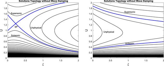
Figure 1. Solution curves expressed as velocity against position for the case of a one-wave system without cosmic-ray diffusion and without wave damping. In this figure, γg = 5/3, γc = 4/3, GM = 1, a = 1, ψB = 1, ψm = 1.2, Ag = 0.5, Ac = 0.5, and  . Left: in a divergent flux-tube geometry with d = 2 and ξd = 1. Right: in a constant flux-tube geometry (or one-dimensional geometry) with d = 0 and ξd = 1. The solutions are divided into subsonic branch, supersonic branch, and unphysical regions (regions where two different velocities occur at the same location in one solution). The blue curves are called transonic solutions. In the divergent flux-tube case (left panel) the two transonic solutions pass through the sonic point, while in the constant flux-tube case (right panel) the two transonic solutions will meet at the sonic point at infinity.
Download figure:
Standard image High-resolution imageIn passing we mention that the corresponding figures for CLWD damping look very similar to Figure 1.
As shown in the right panel of Figure 1, the velocity profile in the subsonic (supersonic) branch increases (decreases) monotonically from the boundary value at the base of the potential well to some asymptotic value at large distances. Clearly, the asymptotic velocity depends on the boundary value of various quantities at the base of the potential well, such as Ub, ρb, Pgb, Pcb,  , Bb, Ψb, etc. To illustrate the idea, suppose an outflow is launched at a height of 1 kpc above the midplane of our Galaxy at the position of the Sun. From Ferrière (2001), at this height the density and pressure of hot gas are ∼0.0065 cm−3 and ∼2 × 10⁻¹² erg cm−3, the pressures of cosmic rays and magnetic field are ∼0.7 × 10⁻¹² erg cm−3 and ∼0.5 × 10⁻¹² erg cm−3, respectively. We adopt the gravitational potential model of the disk by Barros et al. (2016) (see Table 3 of their paper). We take the distance of the Sun from the center of the Galaxy as ∼8.5 kpc. If we pick the units for pressure, density, and velocity as 10−12 erg cm−3, 10−26 g cm−3 and 100 km s−1, respectively, then ρb = 1, Pgb = 2, Pcb = 0.7,
  , and Ψb = −2.4. We plot the asymptotic velocity
  against the velocity at the base Ub in the left panel of Figure 2. In the figure, the dashed, long-dashed, and solid lines correspond to
  and 0.5, respectively. The blue ones belong to the subsonic branch and the red ones to the supersonic branch. The region between them corresponds to those values of velocity at the base that give unphysical solutions. This region will be larger if the potential well is deeper.
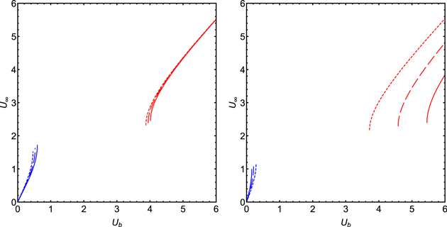
Figure 2. Asymptotic velocity vs. velocity at the base of the potential well. The subsonic branch is blue and the supersonic branch is red. The parameters used in both panels are γg = 5/3, γc = 4/3, d = 0, ξd = 1, Ψb = −2.4, and  . Left: the case of a one-wave system (i.e., three-fluid model) without diffusion and without wave damping (see Sections 3.3 and 4.1). The boundary conditions are ρb = 1, Pgb = 2, and Pcb = 0.7. Right: the case of quasi-thermal outflow without wave damping (see Section 4.3). The boundary conditions are ρb = 1, Pgb = 2, and
  . In both panels, the dashed, long-dashed, and solid lines correspond to forward wave pressures at the base of
  , and 0.5 respectively.
Download figure:
Standard image High-resolution imageWe point out that the case of a backward propagating wave is more complicated because solutions for super-Alfvénic flow and sub-Alfvénic flow can be qualitatively different (as indicated by the lower sign in the above expressions). For instance, it can be shown from Equation (6) that the contribution of the wave damping term  to
to  is positive for sub-Alfvénic flow. Note also that the energy flux of a backward propagating wave is in the negative ξ-direction if MA < 2/3.
In the following discussions on one-wave systems, we focus on a forward propagating wave only. Moreover, we consider super-Alfvénic flow only.
4. Possible Cases
Outflows with cosmic rays and waves can be considered in models of different sophistication, from a one-wave system without diffusion and without wave damping to a two-wave system with diffusion and wave damping. In this section, we compare results of different models with the same boundary conditions at the base of the potential well, e.g., the conditions at the galactic disk for outflow into the galactic halo. Although there are many cases worth discussing, for simplicity, we restrict ourselves mainly to constant flux-tube geometry. Physically allowable solutions refer to those having finite velocity and pressures at large distances. We compare a one-wave system (specifically, a forward propagating wave system) with and without cosmic-ray diffusion and with and without wave damping, for both the subsonic and supersonic branches. Moreover, we also compare results for a two-wave system to those for a one-wave system.
For two-wave systems, we adopt the following working model for e±, κ, and 1/τ (e.g., Skilling 1975; Ko 1992):
where ν± are the collision frequencies of cosmic rays with forward and backward propagating waves. We take  .
.
Besides CLWD damping described in Section 3.2, one can consider other wave damping mechanisms, such as ion–neutral friction (INF) or nonlinear Landau damping (NLLD). Approximately, in terms of the present variables,  for INF, and
  for NLLD (e.g., Kulsrud 2005).
In the following we will discuss a number of cases in three categories. For convenience, we summarize the parameter sets corresponding to different cases (Figures 3–8) in Table 1.
Table 1.
Parameters in Figures 3–8. γg = 5/3, γc = 4/3, GM = 1, a = 1, 
| Figures | Branch | Ub | Pgb | Pcb |

|

|
NLLD (δ±) | Diffusion (κ) |
|---|---|---|---|---|---|---|---|---|
| 3 | Subsonic | 1.2 | 3 | 1 | 0.25 | 0 | 1 | 0 |
| Supersonic | 4 | 3 | 1 | 0.25 | 0 | 1 | 0 | |
| 4 | Subsonic | 1.2 | 3 | 1 | 0.25 | 0 | 1 | κ* |
| Supersonic | 4 | 3 | 1 | 0.25 | 0 | 1 | κ* | |
| 5 | Subsonic | 1.2 | 3 | 1 | 0.25 | 0, 0.125 | 0 | 0, κ*, κ** |
| Supersonic | 4 | 3 | 1 | 0.25 | 0, 0.125 | 0 | 0, κ*, κ** | |
| 6 | Subsonic | 1.2 | 3 | 1 | 0.25 | 0, 0.125 | 1 | 0, κ*, κ** |
| Supersonic | 4 | 3 | 1 | 0.25 | 0, 0.125 | 1 | 0, κ*, κ** | |
| 7 | Subsonic | 1.2 | 5 | 1 | 0.25 | 0 | 0 | 0, κ* |
| Supersonic | 4 | 1 | 1 | 0.25 | 0 | 0 | 0, κ* | |
| 8 | Subsonic | 1.2 | 5 | 1 | 0.25 | 0 | 0, 1, 2 | κ* |
| 1.2 | 5 | 0.2, 0.5, 1 | 0.25 | 0 | 1 | κ* | ||
| 1.2 | 5 | 1 | 0.15, 0.25, 0.35 | 0 | 1 | κ* | ||
| Supersonic | 4 | 1 | 1 | 0.25 | 0 | 0, 1, 2 | κ* | |
| 4 | 1 | 0.2, 0.5, 1 | 0.25 | 0 | 1 | κ* | ||
| 4 | 1 | 1 | 0.15, 0.25, 0.35 | 0 | 1 | κ* | ||
Note.  (for a one-wave system);
  (for a two-wave system).
Download table as: ASCIITypeset image
4.1. One-wave Systems without Diffusion
First, let us consider typical cases of a system with one forward propagating wave without cosmic-ray diffusion and in constant flux-tube geometry (i.e., d = 0 in Equation (30)). In general, physically allowable solutions can be divided into two branches: subsonic and supersonic (see the right panel of Figure 1). We would like to compare velocity and pressure profiles of different cases (say, with and without wave damping) of the same boundary conditions,  at ξb (the base of the potential well). Thus they have the same mass flow rate and magnetic flux, ψm and ψB (note that
  ), and also the same energy constant
  .
.
It can be shown from Equations (27) and (28) that when compared with the case of no wave damping we have the following:
- 1.if γg > 3/2 for the super-Alfvénic regime (MA > 1), or if γg > 5/4 for the sub-Alfvénic regime (MA < 1):
- (a)subsonic branch: CLWD and other wave damping mechanisms (e.g., INF, NLLD) increase U and Pg and decrease Pc and

- (b)supersonic branch: CLWD increases U and and decreases Pg and Pc, while other wave damping mechanisms decrease U and and increase Pg and Pc;
- 2.if γg < 5/4 for the super-Alfvénic regime, or if γg is close enough to one for the sub-Alfvénic regime:
- (a)subsonic branch: CLWD and other wave damping mechanisms decrease U and and increase Pg and Pc;
- (b)supersonic branch: CLWD decreases U and Pg and increases Pc and, while other wave damping mechanisms increase U and Pg and decrease Pc and .


Figure 3 shows the cases of γg = 5/3. The upper row of the figure is the subsonic branch and the lower row is the supersonic branch. In each row the profiles of velocity and pressures of three cases are shown: (1) without wave damping  (no WD, solid line), (2) with completely local wave dissipation
  (CLWD, dashed line), and (3) with nonlinear Landau damping
  (NLLD, dotted–dashed line). We choose GM = 1 and a = 1 in Equation (30) for the potential, and pick ξb = 0 as the base of the potential well.
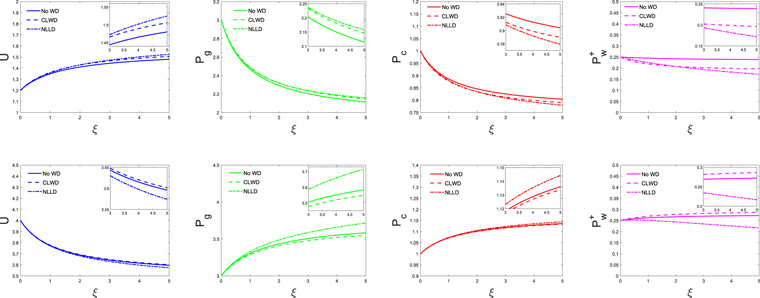
Figure 3. Profiles of outflow of a one-wave system without cosmic-ray diffusion. In this example, γg = 5/3, γc = 4/3, GM = 1, a = 1, and  .
.  for nonlinear Landau damping (NLLD). Upper row: subsonic branch with boundary conditions
  , Ub = 1.2, Pgb = 3, Pcb = 1, and
  . Lower row: supersonic branch with boundary conditions
  , Ub = 4, Pgb = 3, Pcb = 1, and
  . The columns from left to right represent velocity, thermal pressure, cosmic-ray pressure, and forward propagating wave pressure. The solid, dashed, and dotted–dashed lines represent no damping (no WD), completely local wave dissipation (CLWD), and nonlinear Landau damping (NLLD), respectively. Some of the profiles closely resemble each other and almost overlap. The insets are enlarged versions of the figures in order to make the differences more discernible.
Download figure:
Standard image High-resolution imageAs shown in the figure, the effect of CLWD on the profiles of velocity and pressures (in comparison with those of the no-damping case) is not that great, in particular for the supersonic branch. On the other hand, NLLD has a comparably larger effect and significantly alters the profile of  . Of course, if we pick a smaller δ+, the effect will be reduced proportionally. Moreover, if we use INF
  (or even a constant damping rate,
  ), the profiles are more or less similar to those of NLLD.
For the convenience of discerning the slight differences between profiles of different cases (especially the supersonic branch), we provide enlarged versions of parts of each profile as insets in Figure 3 (and Figures 4–8 as well).
4.2. Cosmic-Ray-accompanied Outflows
When cosmic-ray diffusion cannot be neglected, one more condition is needed besides the boundary conditions  mentioned in Section 4.1. We are only interested in physically allowable solutions, thus the extra condition is simply the requirement of finite velocity and pressures at large distances. This requirement imposes restrictions on the cosmic-ray pressure gradient (or the cosmic-ray diffusive flux) at ξb. It turns out that, depending on the parameters, the requirement has two rather distinct possible outcomes. We will discuss these two categories in separate subsections. In the first category (which we call cosmic-ray-accompanied outflow and study in this subsection), the requirement demands a specific value of cosmic-ray pressure gradient at ξb for a given set of
  . The resulting solution is unique. In the second category (which we call quasi-thermal outflow and discuss in Section 4.3), the requirement allows a range of cosmic-ray pressure gradient at ξb for a given set of
  . As a result, there is a set of solutions satisfying the same given set of boundary conditions
  .
.
Once again we would like to compare results of different cases (with and without diffusion, or with and without wave damping). Now the cosmic-ray pressure gradient at ξb will not be the same for different cases. While ψm and ψB (or  ) are the same for different cases,
  is not the same because they will have different cosmic-ray energy diffusive flux (
 ).
).
Here we discuss solutions of the parameter regime in the first category. Figure 4 shows the cases with  and γg = 5/3. All the other parameters and boundary conditions are the same as in Figure 3. To ensure a physically allowable solution, dPc/dξ at ξb is suitably adjusted in each case. As a result
  is slightly different in each case. In general, the trend is the same as the cases without diffusion (see Figure 3). If we use a constant diffusion coefficient, say κ = 1/3, the resulting profiles are very similar to those of Figure 4.
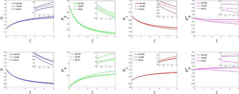
Figure 4. Profiles of outflow of a one-wave system with cosmic-ray diffusion. In this example,  , and γg = 5/3, γc = 4/3, GM = 1, a = 1, and
  . δ+ = 1 for NLLD. Upper row: subsonic branch with boundary conditions
  , Ub = 1.2, Pgb = 3, Pcb = 1, and
  . Lower row: supersonic branch with boundary conditions
  , Ub = 4, Pgb = 3, Pcb = 1, and
  . The columns from left to right represent velocity, thermal pressure, cosmic-ray pressure, and forward propagating wave pressure. The solid, dashed, and dotted–dashed lines represent no damping, completely local wave dissipation, and nonlinear Landau damping, respectively. The insets are enlarged versions of the figures in order to make the differences in profiles more discernible.
Download figure:
Standard image High-resolution imageIn Figure 5, we compare the result of a one-wave system without wave damping and without cosmic-ray diffusion to the same system but with diffusion (i.e., compare the solid lines of Figures 3 and 4). In the figure, solid and dashed lines correspond to the one-wave system without and with diffusion. They both have the same boundary conditions  at ξb, except dPc/dξ. As shown in the figure, in the subsonic branch (upper row), the system with diffusion has larger U, smaller Pg, larger Pc, and smaller
  . In the supersonic branch (lower row), the system with diffusion has larger U, smaller Pg, smaller Pc, and larger
  (cf., e.g., Wiener et al. 2017).
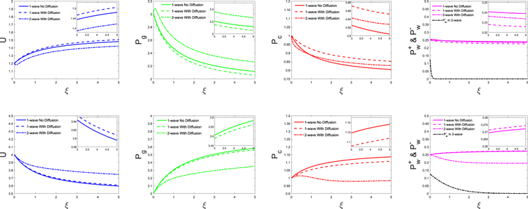
Figure 5. This is an example of different systems without wave damping. Here the solid, dashed, and dotted–dashed lines represent the one-wave system without diffusion, the one-wave system with diffusion, and the two-wave system with diffusion, respectively. The black dotted–dashed curve in the rightmost column denotes backward propagating wave pressure for the two-wave system. In this example, γg = 5/3, γc = 4/3, GM = 1, a = 1, and  . Upper row: subsonic branch with boundary conditions
  , Ub = 1.2, Pgb = 3, Pcb = 1, and
 for the one-wave systems and
  for the two-wave system. Lower row: supersonic branch with boundary conditions
  , Ub = 4, Pgb = 3, Pcb = 1, and
 for the one-wave systems and
  for the two-wave system. The insets are enlarged versions of the figures in order to make the differences in profiles more discernible.
Download figure:
Standard image High-resolution imageWe also give an example of a two-wave system in Figure 5 for comparison. The two-wave system adopts Equation (31) (with  ) and has the same boundary conditions
  as the one-wave system, but with an extra condition
  for both subsonic and supersonic branches. As shown in the figure, there are notable differences in the subsonic branch, but only tiny differences in the supersonic branch. The insets in the figure are enlarged versions underscoring the differences. The upper row of Figure 5 shows that in the subsonic branch, the velocity of the two-wave system with
  is smaller (while the thermal pressure is larger) with respect to the one-wave system without diffusion. In fact, in this case as
  increases from 0 (one-wave system) to 0.125, the profile of U (Pg) decreases (increases) from above (below) the case without diffusion to below (above) it. On the other hand, in the supersonic branch, the profile of U (Pg) increases (decreases) further from above (below) the case without diffusion as
  increases from 0 to 0.125.
Figure 6 is the same as Figure 5 except that the NLLD wave damping mechanism is considered ( ).
).
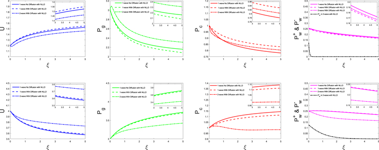
Figure 6. This is an example of different systems with nonlinear Landau damping. Here the solid, dashed, and dotted–dashed lines represent the one-wave system without diffusion, the one-wave system with diffusion, and the two-wave system, respectively. The black dotted–dashed curve in the rightmost column denotes backward propagating wave pressure for the two-wave system. In this example, γg = 5/3, γc = 4/3, GM = 1, a = 1,  , and
, and  . Upper row: subsonic branch with boundary conditions
  , Ub = 1.2, Pgb = 3, Pcb = 1, and
 for the one-wave systems and
  for the two-wave system. Lower row: supersonic branch with boundary conditions
  , Ub = 4, Pgb = 3, Pcb = 1, and
 for the one-wave systems and
  for the two-wave system. The insets are enlarged versions of the figures in order to make the differences in profiles more discernible.
Download figure:
Standard image High-resolution image4.3. Quasi-thermal Outflows
Here we discuss solutions of the parameter regime in the second category mentioned in Section 4.2. This is the regime where the waves in the system wither (through streaming instability, stochastic acceleration, or other damping mechanisms). When waves die cosmic rays will be decoupled from the thermal gas (the diffusion coefficient becomes infinite, see Equation (31)), and the outflow becomes a thermal outflow, which we called quasi-thermal outflow.
For the purpose of illustration, we consider systems with  . Suppose at large distances (subscript a) the wave pressures vanish and cosmic rays are decoupled from the thermal gas, then the energy constant
  of the quasi-thermal wind is

As  , thus
  (Equation (12)). As the waves wither at large distances, the cosmic-ray flux at large distances is related to the boundary conditions by the wave action integral, Equation (13):
Hence
where Ucrit is given by Equation (A2). By the argument given in the Appendix, the boundary conditions for a physically allowable solution for the quasi-thermal outflow are constrained by (see Equation (A5) and the argument that follows)

If this criterion is satisfied, then the asymptotic velocity  is given by Equations (32) and (34). It is interesting that the criterion and the asymptotic velocity are independent of Pcb (and its gradient).
The dependence of the asymptotic velocity of the quasi-thermal outflow on the boundary value at the base of the potential well is shown in the right panel of Figure 2. This is the same example described near the end of Section 3 on an outflow from 1 kpc above the midplane of our Galaxy, except that the model for the outflow is different. Recall that if the units for pressure, density, and velocity are 10−12 erg cm−3, 10−26 g cm−3, and 100 km s−1, the values at the base of the potential well are ρb = 1, Pgb = 2,  ,
,  , and Ψb = −2.4. The dashed, long-dashed, and solid lines correspond to
  and 0.5, respectively. As shown in the figure, the supersonic branch in the case of quasi-thermal outflow is more sensitive to
  than in the case of a one-wave system (i.e., three-fluid model) without diffusion.
Figure 7 shows the profiles of a one-wave system (forward propagating wave) with  . The upper row is an example of a subsonic flow and the lower row a supersonic flow. The left column shows the velocity profile and the right column the pressure profiles. The dotted–dashed line is the quasi-thermal outflow (diffusive case). For comparison we show the one-wave system without diffusion (see Section 4.1) as a solid line. Both cases have the same boundary conditions
  at ξb (the only difference is that the one system has diffusion and the other does not). In the figure, we also show the pure thermal outflow with the same boundary conditions {Ub, Pgb, ρb, Bb} (dashed line).
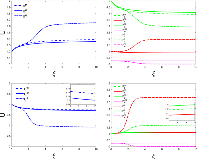
Figure 7. Comparison of one-wave quasi-thermal outflow with the one-wave system without diffusion in the parameter regime in the first category. Both cases are without wave damping. In this example, γg = 5/3, γc = 4/3, GM = 1, a = 1, and  . Upper row: subsonic branch with boundary conditions
  , Ub = 1.2, Pgb = 5, Pcb = 1, and
  . Lower row: supersonic branch with boundary conditions
  , Ub = 4, Pgb = 1, Pcb = 1, and
  . Velocity profiles are shown in the left column and pressure profiles in the right column. The dotted–dashed and solid lines denote quasi-thermal outflow and the one-wave system without diffusion, respectively. In addition, dashed lines show the profiles of velocity and thermal pressure of pure thermal outflow with Ub = 1.2 and Pgb = 5 in the subsonic branch, and Ub = 4 and Pgb = 1 in the supersonic branch. Note that in the supersonic branch the solid line almost overlaps the dashed line. The insets are enlarged versions of the figures to emphasize the slight differences between the profiles in the supersonic branch.
Download figure:
Standard image High-resolution imageOne can see in the subsonic flow that the diffusive case follows the non-diffusive case near the base. Somewhere along the flow a transition occurs: the diffusive case diverges from the non-diffusive case. The wave dies, the cosmic-ray pressure increases (and becomes constant), the thermal pressure decreases, the velocity increases, and the flow becomes a quasi-thermal outflow. For the case with diffusion, the cosmic-ray pressure gradient at the base must be larger than a specific minimum value to have physically allowable solutions. When we tune the cosmic-ray pressure gradient at the base from the minimum value to some larger values the transition region occurs closer and closer to the base, but the asymptotic velocity and thermal pressure ( and Pg∞) do not change. The asymptotic cosmic-ray energy flux changes according to the change in diffusive flux at the base. Supersonic flow has similar behavior, except that in the transition region the thermal pressure increases while the velocity decreases.
If  (e.g., with INF or NLLD), the system is more complicated and cannot be analyzed as nicely as the case of
  . In any case, parameter regions for quasi-thermal outflow exist. However, in contrast to the simple case of no wave damping, the asymptotic velocity and thermal pressure depend on the cosmic-ray pressure (and its gradient) at the base, and of course on the strength of damping (δ±).
An example of a one-wave quasi-thermal outflow with NLLD is shown in Figure 8. (In fact, the result is qualitatively the same with INF or a constant damping rate.) The figure illustrates how the velocity profile is affected by changing δ+, Pcb, and  . In the subsonic branch, as δ+ increases, the velocity becomes smaller (except in regions close to the base, in which the velocity becomes larger by a small amount). As Pcb or
  increases, the velocity becomes larger. In the supersonic branch, as δ+ increases, the velocity becomes larger (but by a minute amount). As Pcb increases, the velocity becomes larger (more noticeable in the transition region but only a small increase at large distances). As
  increases, the velocity becomes quite a lot smaller.
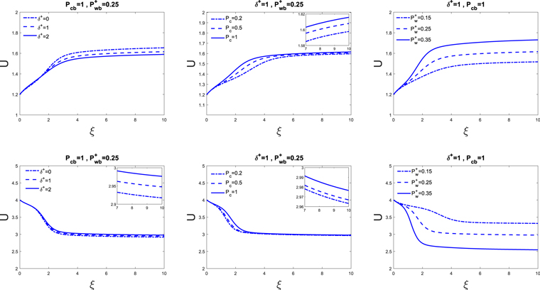
Figure 8. Velocity profiles of one-wave quasi-thermal outflow with nonlinear Landau damping. In this example, γg = 5/3, γc = 4/3, GM = 1, a = 1, and  . Upper row: subsonic branch boundary conditions
  , Ub = 1.2, Pgb = 5, κdEc/dξ = 0. Lower row: supersonic branch boundary conditions
  , Ub = 4, Pgb = 1, κdEc/dξ = 0.4. Different profiles correspond to different δ+, Pcb, and
  (see annotation in the figures for the values, or see Table 1). The insets are enlarged versions of the figures to emphasize the slight differences between the velocity profiles.
Download figure:
Standard image High-resolution imageThe characteristic of the outflows described in this section is that they becomes pure thermal outflows at large distances. If cooling is not negligible then the thermal outflow or wind will be significantly affected. For instance, if we consider cooling only (and nothing else) then a one-dimensional subsonic flow will stall (see the Appendix). However, it is well known that if other effects are included then one-dimensional thermal wind can have interesting flow profiles, such as transonic solutions (see, e.g., Bustard et al. 2016). The models described here (with wave damping or not) also possess transonic solutions. A systematic and thorough discussion of these possible solutions warrants further investigation in the future.
5. Summary and Discussion
We study plasma outflow from a gravitational potential well with cosmic rays and self-excited Alfvén waves. We explore models of different levels of complexity. The most complicated model is the four-fluid system (also called the two-wave system), which comprises thermal plasma, cosmic rays, and forward and backward propagating Alfvén waves, with wave damping (such as stochastic acceleration, ion–neutral friction, nonlinear Landau damping). In principle, outflow or wind is driven by various pressure gradients against gravity (e.g., Equation (3)). Yet there are intricate interactions between the components. In general it is difficult to analyze the four-fluid system analytically even in the so-called flux-tube formation (i.e., assume a prescribed magnetic flux tube and the flow moves along the tube). However, for simpler systems some analytical work can be done.
We start from the simplest system we have: the three-fluid system (or one-wave system) without diffusion of cosmic rays in the flux-tube formulation. In this system we consider only forward propagating wave and assume zero cosmic-ray diffusion coefficient. The system can be analyzed in exactly the same way as the classic Parker's stellar wind (Parker 1958). The outflow velocity can be expressed (implicitly) in terms of ξ, the coordinate along the flux tube. Both panels of Figure 1 show the solution curves of the outflow. For convenience we focus on the one-wave system (forward wave) in constant flux-tube geometry (the right panel of Figure 1). We are interested in physically allowable solutions (i.e., where quantities have finite values at large distances). Figure 3 shows the solution profiles of a typical set of boundary conditions  at ξb (the base of the potential well). For the case without wave damping, whether the set of boundary conditions can give a physically allowable solution or not can be studied by a method similar to that in the Appendix. Moreover, if wave damping is included, the velocity (and other quantities) may increase or decrease depending on whether the solution is subsonic or supersonic, sub-Alfvénic or super-Alfvénic, and also on some other parameters (for details, see Section 4.1).
If cosmic-ray diffusion cannot be neglected in the one-wave system, things become more interesting. Cosmic-ray diffusion is facilitated by waves, thus we take the diffusion coefficient to be inversely proportional to the wave energy density (or pressure). Since diffusion is considered, one more condition is needed in addition to the boundary conditions mentioned above. We simply insist on physically allowable solutions (i.e., finite value at large distances). There are two main categories of solutions: (1) cosmic-ray-accompanied outflow (solutions closely resemble those without diffusion) and (2) quasi-thermal outflow.
In the first category, the requirement of finite values at large distances demands a specific cosmic-ray pressure gradient at the base of the potential well (and all other values of the gradient give unphysical solutions), see Figures 4, 5, and 6. The one-wave system with diffusion has a larger velocity than that without diffusion in both subsonic and supersonic branches (but only a tiny difference is observed in the supersonic branch). The one-wave system is a special case of the two-wave system (four-fluid system). If we increase the amount of backward propagating waves at the base of the potential well, the velocity (thermal pressure) will decrease (increase) accordingly in the subsonic branch, but there is no systematic trend in the supersonic branch (anyway, the difference is minor in this branch). A more detailed description is presented at the end of Section 4.2.
In the second category, the waves vanish at large distances and the cosmic rays are decoupled from the thermal plasma (as the diffusion coefficient becomes extremely large). The flow acts like a pure thermal outflow. A range of cosmic-ray pressure gradients at the base of the potential well can give a finite value at large distances. Basically, the solution acts like an outflow similar to the solutions of the first category then undergoes a transition to a thermal outflow at large distances, see Figure 7.
Now, if there is no extra wave damping ( ), we can be more specific about these two categories. If the boundary conditions
  satisfy/violate Equation (35), then the solutions belong to the second/first category (see Section 4.3). Moreover, if Equation (35) is satisfied, the asymptotic velocity (velocity at large distances) is given by Equation (32). The interesting fact is that this asymptotic velocity is independent of cosmic-ray pressure (and its gradient) at the base of the potential well. Nevertheless, if
  , this independence of cosmic rays no longer holds. (An example of a one-wave system with NLLD is given at the end of Section 4.3.)
To this end, we would like to address the question of the consequence of adding cosmic rays to a thermal outflow. This depends on the system. Suppose there is a thermal outflow with boundary conditions {Ub, Pgb, ρb, Bb}. The corresponding asymptotic velocity  is obtained from its energy constant (see Equation (A3)). Now cosmic rays and waves (
 ) are added into the system. Once again for convenience we consider a one-wave system without wave damping (
 ,
,  ). First, for the non-diffusive case, the asymptotic velocity
  can be found from the energy constant in Equation (11). It turns out that for most parameters (at least for Pcb and
  from close to zero to the order of Pgb),
  is smaller than
  by a small amount in the subsonic branch, and by a very tiny amount in the supersonic branch. If diffusion of cosmic rays cannot be ignored and the boundary conditions belong to the first category, the result is similar to the non-diffusive case. However, it is more interesting if the boundary conditions belong to the second category (the quasi-thermal case). The asymptotic velocity
  is given by the energy constant in Equations (32) and (34). In this case,
  in the subsonic branch and
  in the supersonic branch. Figure 7 shows an example of one of these cases. We note that an exposition of this question from other perspective is given in the Appendix.
B.R. and C.M.K. are supported in part by the Taiwan Ministry of Science and Technology grants MOST 105-2112-M-008-011-MY3, MOST 108-2112-M-008-006, and MOST 109-2112-M-008-005. D.O.C. is supported by the grant RFBR 18-02-00075 and by foundation for the advancement of theoretical physics "BASIS."
Appendix: Thermal Outflows
In this appendix we revisit the classical thermal outflow or wind in a potential well. We examine the characteristic of the solution from a given set of boundary conditions at the base of the potential well. Specifically, we study the constraint on the velocity at the base in order to have a physical outflow solution when the thermal pressure at the base is given.
For simplicity, we consider polytropic gas in a one-dimensional geometry (flow tube of constant area, i.e., Δ is a constant). The wind equation is

where M = U/ag,  , and
, and  is the mass flux, which is a constant in one-dimensional flow. Note that the mass flow rate
  . Ψ is the potential well, which is a monotonically increasing function of ξ from the base of the potential well ξb to
  . We set Ψ = 0 as
  , thus Ψ ≤ 0. Suppose at the base of the potential well, U = Ub, ρ = ρb, Pg = Pgb (and
  ), and for convenience we call these "boundary conditions."
The sonic point of the system is located at  or Ψ = 0, and the critical velocity is given by
  , or
, or
The solution to the wind equation can be expressed in terms of an integral, the energy constant:
and for polytropic gas γg > 1. The corresponding energy constant for the transonic solution is
Equations (A3) and (A4) give the constraint on the boundary conditions for a possible transonic solution,
In Figure 9 the blue and red (dashed) curves are the plots of the left-hand side of Equation (A5) as a function of Ub. Pgb and ρb are given in the left panel and Pgb and  in the right panel. We set Ψb = −1 as the base of the potential well, marked by the long-dashed orange line in the figure. The intersections of the curves and the long-dashed orange line are the values of the velocity at the base (Ub) that give rise to transonic solutions. For physically allowable solutions (i.e., solutions that extend to large distances or Ψ = 0),
  . Thus, the ranges of Ub in which the curve is above the long-dashed orange line are those boundary conditions that correspond to physically allowable solutions. The range with smaller Ub is subsonic and that with larger Ub is supersonic.
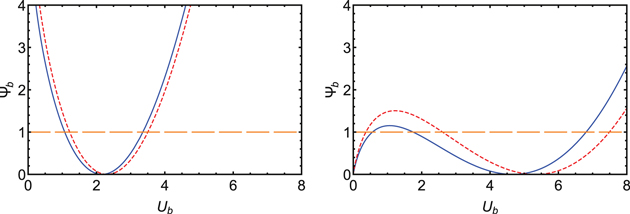
Figure 9. Constraint on velocity Ub at the base of the potential well Ψb. The long-dashed orange line represents −Ψb. Left: {Pgb, ρb} = {2.8, 1} and {Pgb, ρb} = {3.2, 1} for the blue curve and dashed red curve, respectively. Right:  and
and  for the blue curve and dashed red curve, respectively. γg = 5/3 for both cases. The intersection of the curve and the long-dashed orange line is the value of Ub that gives rise to a transonic solution.
Download figure:
Standard image High-resolution imageIn the figure, Pgb of the red dashed curve is larger than that of the blue curve. As shown in the figure, the range of the subsonic/supersonic branch of the red dashed curve is larger/smaller than that of the blue curve. Thus for subsonic/supersonic solutions close to transonic solution, decreasing/increasing Pgb (but keeping Ub and ρb fixed) nudges the solution to an unphysical regime.
In the case of given Pgb and  (right panel of the figure), there is only a supersonic branch if Pgb is small enough, or
  is large enough, or the potential well is deep enough (i.e., more negative Ψb). In the case of given Pgb and ρb (left panel of the figure), there is always a subsonic branch and a supersonic branch if
  , otherwise there is only a supersonic branch.
Similar analysis can be applied to the one-wave system without cosmic-ray diffusion described in the main text. As expected, a similar conclusion is obtained. We would like to know the consequence of adding cosmic rays to a thermal wind. This depends on how we frame the question.
- 1.Prescribed Pgb, ρb, Ub (i.e., the mass flux is fixed also).If the thermal wind is in the supersonic region and is close to a transonic solution, then adding (a small amount of) cosmic rays may nudge it toward the unphysical regime. On the other hand, if the thermal wind is in the subsonic region but within the unphysical regime, then adding cosmic rays may push the flow to enter the physically allowable regime.
- 2.Prescribed Pgb, ρb, but Ub is allowed to change (i.e., the mass flux can be adjusted).Suppose the thermal wind is at a transonic solution. Now add (a small amount of) cosmic rays and then seek a new transonic solution. The new Ub (and the profile as well) will be higher.


Suppose cooling is significant and cannot be neglected in the flow, then Equation (A1) should be replaced by

where Γ < 0 for cooling. For example, for radiative cooling  , where T ∝ Pg/ρ is temperature. When cooling (and heating for that matter) is not negligible, the integral energy constant
  no longer exists. However, if gravity can be neglected (e.g., at a large distances from the base of the potential well), then the total momentum is conserved in one-dimensional flow,

The Mach number becomes
and M is a monotonically increasing function of U for 0 ≤ U < G'. Moreover, T ∝ U(G' − U), i.e.,  as
as  or G'.
For cooling, Γ < 0 and the right-hand side of Equation (A7) is positive if gravity is negligible. Therefore, in the subsonic regime, dU/dξ < 0. The velocity decreases monotonically along the flow and the flow becomes more and more subsonic (see Equation (A9)). Eventually,  and
and  (and
(and  ). The flow will stall, unless Γ vanishes before U = 0.
On the other hand, in the supersonic regime, dU/dξ > 0. The velocity increases monotonically along the flow and the flow becomes more and more supersonic. Eventually,  and
and  (and
(and  ). The flow will be unphysical because the thermal pressure will become negative (see Equation (A6)), unless Γ vanishes before U = G'.
Now let us put gravity back into consideration. If the gravity is strong enough, then it is possible that the right-hand side of Equation (A7) is negative near the base and positive at large distances, i.e., it is zero at some finite distance. Thus, it is conceivable that a sonic point exists at a finite distance (the right-hand side of Equation (A7) vanishes together with M = 1). Therefore, transonic solutions are possible.