


Abstract
We address the very large diversity of jet production efficiency in active galactic nuclei (AGNs) by using data on low-redshift AGNs selected from the Swift/BAT catalog and having black hole (BH) masses larger than 108.5 M⊙. Most of these AGNs accrete at intermediate rates and have bolometric luminosities dominated by mid-IR radiation. Our sample contains 14% radio-loud (RL), 6% radio-intermediate, and 80% radio-quiet (RQ) AGNs. All RL objects are found to have extended radio structures, and most of them have classical FR II morphology. Converting their radio loudness to jet production efficiency, we find that the median of this efficiency is on the order of ( d/0.1)%, where
  is the radiation efficiency of the accretion disk. Without knowing the contribution of jets to the radio emission in RQ AGNs, we are only able to estimate their efficiencies using upper limits. Their median is found to be 0.002(d/0.1)%. Our results suggest that some threshold conditions must be satisfied to allow the production of strong, relativistic jets in RL AGNs. We discuss several possible scenarios and argue that the production of collimated, relativistic jets must involve the Blandford–Znajek mechanism and can be activated only in those AGNs whose lifetime is longer than the time required to enter the magnetically arrested disk (MAD). Presuming that MAD is required to collimate relativistic jets, we expect that the weak nonrelativistic jets observed in some RQ AGNs are produced by accretion disks rather than by rotating BHs.
Export citation and abstract BibTeX RIS
1. Introduction
While the first quasars were discovered following the identification of some radio sources with optical point sources located at cosmological distances (Schmidt 1963), it quickly turned out that most of them were radio quiet (RQ; Sandage 1965). This led to their division into radio-loud quasars (RLQs) and RQ quasars (Kellermann et al. 1989) with an approximate number proportion 1:10. However, later studies using deeper radio surveys led to the discovery of many quasars with intermediate radio loudness, and the often-claimed radio bimodality came into question (see Kratzer & Richards 2015, and references therein).
A broad distribution of radio loudness was also found in active galactic nuclei (AGNs) located at much closer distances than luminous quasars (e.g., Rafter et al. 2009), and if the dominating radio flux of the extended radio sources with which they were associated was included, the bimodality reappeared (Rafter et al. 2011). A bimodal radio distribution in AGNs was also confirmed by the recent studies of Gupta et al. (2018, 2020). In order to avoid biases in the determination of the radio-loudness distribution associated with optical and radio selection limits, Gupta et al. based their studies on a sample of AGNs selected from the Swift/BAT catalog (Ricci et al. 2017). Due to the very low sensitivity of the BAT detector, most of these AGNs are located at low redshift. The radio-loudest AGNs were found, like in quasars, in AGNs with MBH > 108M⊙, but with much lower accretion rates. The latter also concerns RQ AGNs with very massive black holes (BHs) and can be explained by the "downsizing effect," according to which the average specific accretion rates in massive AGNs decrease with decreasing redshift (e.g., Fanidakis et al. 2012). In order to minimize the impact of RL and RQ AGNs having different average BH masses and Eddington ratios ( ) on the compared radio properties, the sample adopted from the Swift/BAT catalog of AGNs was reduced to have RQ and RL AGNs with similar ranges of these parameters.
The advantages of studying the radio properties of AGNs and possible relations to the optical properties of their host galaxies and environments using the low-redshift samples are obvious: (1) almost all of these AGNs have radio detections, (2) studies of radio morphology are not limited to only extended radio sources, (3) studies of optical morphology of their hosts and environment are possible, (4) biases associated with cosmological evolution are minimized, and (5) a much lower probability of having radio-intermediate (RI) AGNs dominated by strong starbursts and accretion disk winds. Hence, studies incorporating such samples have exceptional potential to provide a variety of constraints that can be used to select the most promising scenario to explain the origin of the large diversity of jet production efficiency.
Our work is organized as follows: in Section 2 the sample is defined; in Section 3 the radio-loudness distribution is derived and radio morphologies are determined; in Section 4 bolometric luminosities, BH masses, Eddington ratios, and jet powers are derived and used to construct the distribution of jet production efficiency; and in Section 5 properties of the host galaxies are reviewed. A comparison of our results with others and their theoretical implications and possible interpretations are provided in Section 6 and summarized in Section 7.
Throughout the paper, we assume a ΛCDM cosmology with  , Ωm = 0.3, and ΩΛ = 0.70.
2. The Sample
Our initial sample is taken from Gupta et al. (2018, 2020), who performed a comparison of RL and RQ, both Type 1 and Type 2, AGNs in various spectral bands. The sources in their sample were selected from the BAT AGN Spectroscopic Survey (Ricci et al. 2017), by excluding blazars, Compton-thick (log NH > 24) AGNs, and sources with missing optical spectroscopic classification in Koss et al. (2017), which resulted in 664 objects. The sample in Gupta et al. (2018) was limited to 70 sources. This was due to the limits imposed on BH masses and Eddington ratios (8.48 ≤ log MBH ≤ 9.5,  ), which gave the authors possibly the best representation of radio galaxies and their RQ counterparts working at intermediate accretion rates. In Gupta et al. (2020), some of the earlier restrictions were relaxed and additionally, using the relation between BH masses and the near-infrared (NIR) luminosities of host galaxies of AGNs (Marconi & Hunt 2003; Graham 2007), the BH masses were calculated. As a result, instead of studying only those sources for which the BH masses are known, the sample studied in Gupta et al. (2020) has 290 objects, all of them with
  , z ≤ 0.35 and
  . Hence, we decided to make use of the sample from Gupta et al. (2020) and complete it by adding RI AGNs (which were excluded by the authors; see Gupta et al. 2018, 2020), choosing them in the same way as the other objects were found. This resulted in finding 24 additional sources (out of which four turned out to be RQ), giving us a final sample consisting of 314 Swift/BAT AGNs.
The detailed description of the data and the procedure used to build this sample, originally described in Gupta et al. (2018, 2020), is reiterated in Appendix A.
3. Radio Properties
3.1. Radio Loudness
Our radio-loudness parameter, as in Gupta et al. (2020), is given as  , where F1.4 and
  are the monochromatic fluxes at 1.4 GHz4
and in the Wide-field Infrared Survey Explorer (WISE) at
are the monochromatic fluxes at 1.4 GHz4
and in the Wide-field Infrared Survey Explorer (WISE) at  Hz, respectively. This relates to the definition given by Kellermann et al. (1989), i.e.,
  , where F5 and
  are the monochromatic fluxes at 5 GHz and in the B band (6.8 × 10¹⁴ Hz), as R ≈ 0.1 × RKL, assuming the spectral indices of α1.4–5 = 0.8 and
  (see Gupta et al. 2018). Based on this, we partitioned the sources into the following radio classes, strictly corresponding to those in Kellermann et al. (1989): RL when R > 10, RI for 1 < R < 10, and RQ when R < 1.
Because we used three radio catalogs differing in radio wavelength, angular resolution, and sensitivity, we decided to adopt the radio flux from the National Radio Astronomy Observatory (NRAO) Very Large Array (VLA) Sky Survey (NVSS), whose data are available for most of the sources and whose sensitivity accounts for all of the extended emission. For objects lacking NVSS data, we took fluxes from the Sydney University Molonglo Sky Survey (SUMSS) and Faint Images of the Radio Sky at Twenty-cm (FIRST).5 Such an approach resulted in finding 44 RL, 20 RI, and 250 RQ AGNs in our sample, with their radio-loudness medians of 75.40, 1.69, and 0.15, respectively. The exact radio-loudness distribution is presented in the top panel of Figure 1.

Figure 1. Radio-loudness distribution for Swift/BAT AGNs in our sample. The top panel shows groups of RL (red), RI (green), and RQ (gray) sources, based on the definition of the radio-loudness parameter given as  , which, for the given classes, takes values of R > 10, 1 < R < 10, and R < 1, with its median value of log R equal to 1.88, 0.23, and −0.84, respectively. In the RQ class, we separate sources with (RQ detected, dark gray, with a median value of log R ≃ −0.75) and without radio detections, dividing the latter group into two categories: RQ undetected with a 2.5 mJy detection upper limit (light yellow) when the source is in the footprint of NVSS or SUMSS, and RQ undetected up to 1.0 mJy (light gray) when the source is in the FIRST area. The middle panel distinguishes between sources with (teal) and without (brown) extended radio emission together with the same groups of RQ undetected AGNs as mentioned earlier. Here the median values of log R are 1.74 and −0.72 for extended and compact AGNs, respectively. The characteristics of these radio morphologies are closely described in Sections 3.2.1 and 3.2.2, and exact numbers are presented in Table 1. The bottom panel shows the sample distribution using two different bin widths in gray and purple. Overplotted are the maximum likelihood estimates for unimodal and bimodal normal distributions in black and red, respectively.
Download figure:
Standard image High-resolution imageAmong 314 Swift/BAT AGNs, 257 of them have and 57 lack radio data. As one can see in Figure 1, those radio-undetected sources belong entirely to the RQ class. In the group of radio-detected objects, we can specify two subsamples of sources for which we have both: (1) NVSS and SUMSS data (12 sources) and (2) NVSS and FIRST data (76 sources). While the NVSS and SUMSS total fluxes (compared at 1.4 GHz) are almost the same, the ratio of NVSS to FIRST total fluxes is slightly more significant, with a median of 1.2, showing that, indeed, some of the faint extended radio emission might be lost while using only higher angular resolution and better sensitivity radio data.
3.2. Radio Morphologies
Within the group of 257 radio-detected AGNs, we can distinguish two main subsamples—those with and without extended radio emission, represented by 52 and 205 objects, respectively. Below we give detailed characteristics of our radio morphological classification.
3.2.1. Compact Sources
Sources belonging to the group of compact AGNs are defined as those for which only one radio match, with its location corresponding to the optical center, was found. Based on whether or not the accurate size of the fitted major axis after deconvolution in a given radio catalog was available, compact sources form two groups: resolved and unresolved, consisting of 91 and 114 sources, respectively.
3.2.2. Extended Sources
All AGNs with more than one confirmed radio match are classified as extended. Based on the appearance of their radio morphologies, this subsample has been divided into the following morphological groups:
- 1.complex, in which we include sources with multiple pairs of lobes, i.e. double–double radio galaxies (DDRG) and X-shaped sources (five sources),6
- 2.triple, when the core and a pair of lobes are clearly visible (20 sources),
- 3.double, objects with a pair of lobes but with no detection of a core corresponding to the optical center (15 sources),
- 4.knotty, sources with quite extended, yet difficult to define, emission present on the radio map (12 sources).
In general, the extended radio emission from AGNs in our sample can be distinguished into sources with (complex, triple, double) and without (knotty) visible radio lobes.
3.2.3. Radio Morphology versus Radio-loudness Classification
Using the above-described division of radio-detected AGNs, we checked how our radio morphological groups relate to the radio-loudness categorization. In Table 1 we list these characteristics. Most of the RL sources are found to have lobed radio morphologies (36 out of 44),7 while almost all RQ objects correspond to compact sources (186 out of 193). In the case of RI objects, the ratio of sources with extended radio emission to those without is 1:3. This shows that the fraction of AGNs with extended radio emission decreases along with their radio loudness, which is not only clearly visible in Figure 1 but is also reflected by the quite similar median values of the radio loudness of RL and extended sources (75.40 and 54.61) and of RQ detected and compact sources (0.18 and 0.19).
Table 1. Radio Morphologies and Radio Classes of Radio-detected Sources (257 Objects) in Our Sample of Swift/BAT AGNs
| Radio Morphology | Radio Class | Total | |||
|---|---|---|---|---|---|
| RL | RI | RQ | |||
| Extended | Complex | 5 | 5 | ||
| Triple | 16 | 4 | 20 | ||
| Double | 15 | 15 | |||
| Knotty | 4 | 1 | 7 | 12 | |
| Compact | Resolved | 4 | 3 | 84 | 91 |
| Unresolved | 12 | 102 | 114 | ||
| Total | 44 | 20 | 193 | 257 | |
Note. A detailed description is given in Section 3.2.
Download table as: ASCIITypeset image
In addition to the above, we analyzed whether a unimodal or bimodal normal distribution best corresponds to our radio-loudness sample. We performed a maximum likelihood estimate to fit the data to the two distributions and then conducted a Kolmogorov–Smirnov test with pvalues of 3.13 × 10⁻¹⁰ and 0.87 for the uni- and bimodal distributions, respectively. We found that while the unimodal distribution differs significantly from the observed sample, the same cannot be said about the bimodal distribution. The fitted distributions are shown on the bottom panel in Figure 1.
3.2.4. FR I/II Classification
For sources with a lobed radio morphology (i.e., complex, triple, and double objects; 40 AGNs total) based on the appearance of their radio maps, we established their Fanaroff–Riley classification (Fanaroff & Riley 1974), finding the following: four objects of type FR I, two AGNs of mixed FR I/II class, and 34 type FR II AGNs. Our classification is in an agreement with the data given in, e.g., Rafter et al. (2011), Kozieł-Wierzbowska & Stasińska (2011), and Panessa et al. (2016).
3.3. Physical Sizes
The (projected) largest linear size (LLS) was determined for each radio-detected source in our sample. Noting that the true definition of LLS is given as the distance between two hot spots, the most reliable calculations are available for sources with double radio lobes. For complex AGNs with multiple pairs of lobes, the pair with the largest separation was used. The sizes of knotty radio sources correspond either to the distances between the most distant radio matches or to our measurements obtained from their radio maps. The sizes of compact AGNs (exact measurements for resolved and upper limits for unresolved objects) were taken directly from the radio catalogs as the major axis of the fitted Gaussian (a detailed procedure for the size estimation of compact AGNs is given in Appendix B).
The results for the LLS calculations for all the radio-detected sources are shown in the left panel of Figure 2. Knowing that only three out of six morphological groups (namely, complex, triple, and double sources) presented in this paper have direct measurements of the projected size and the sizes of compact (unresolved and resolved) and knotty sources are upper limits (i.e., are possibly shifted to the left on this chart), a clear trend confirming our results from Section 3.2.3 is found, namely, the most extended AGNs are RL whereas the RQ ones do not achieve such big sizes. This distinction is especially visible in the right panel of Figure 2, where only compact sources with radio data from FIRST (which, within the group of 57 compact sources, provides more precise, and is on average 15 times smaller sizes than NVSS; see Appendix B) are included. This figure shows that compact resolved and compact unresolved objects are in fact located in different parts of the diagram.
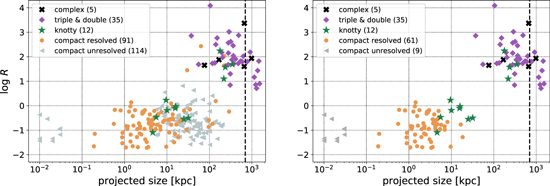
Figure 2. Distribution of radio-detected sources in the log R vs. projected size plane. Morphological groups are presented as follows: complex correspond to black crosses, triples and doubles are presented together as purple diamonds, knotty objects are marked as green stars, and the group of compact resolved sources is shown as orange circles while compact unresolved ones correspond to gray triangles. The left panel presents all radio-detected objects (257 AGNs). Compact sources on the right panel have been limited to those with FIRST data used (122 AGNs total), which allow a clear separation to be seen between resolved and unresolved objects. Nine of our sources have sizes corresponding to GRGs and those are located to the right of the vertical dashed line marking the size of 700 Mpc.
Download figure:
Standard image High-resolution imageFrom Figure 2 we note that nine sources have projected sizes beyond 700 kpc, which is the definition of giant radio galaxies (GRGs). The fraction of GRGs in our sample compared to the total number of lobed sources (9/40 ≈ 23%) is almost the same as in Bassani et al. (2016), where the authors found that 14 out of their 64 confirmed radio galaxies selected in the soft gamma-ray band and having double-lobe morphologies have giant sizes. Furthermore, Bruni et al. (2019) found that 61% of Bassani et al. giant radio sources have a gigahertz-peaked spectrum (GPS) cores, i.e., young nuclei. We checked that all of our GRGs are in common with those studied by Bruni et al. (2019), with six of them (67%) having GPS cores suggesting the ongoing accretion and reactivation of the jets.8 By contrast, four of their AGNs are not found in our sample as they were not observed by Swift/BAT or have blazar-like nuclei, while another two sources (namely 4C +63.22 and PKS 2356–61) listed in Bruni et al. are not recognized as GRGs because their sizes, estimated in this work, are slightly below 700 kpc.
4. Jet Production Efficiency
4.1. Bolometric Luminosity
We started our calculations of bolometric luminosity by checking whether or not the method in which MIR W3 fluxes were used to estimate Lbol, as was done in Gupta et al. (2018), can be successfully applied to our sample of AGNs accreting at a moderate accretion rate. Such verification was possible due to the accessibility of the multiband spectra, and in turn, the exact values of bolometric luminosities, which are presented in Gupta et al. (2020), upon which we built our sample of Swift/BAT AGNs.
We decided to analyze a subsample consisting of 131 (20 RL, 111 RQ) sources—all of those being Type 1 and having strict MIR, NIR, optical-UV, and hard X-rays detections (for more details, see Section 4 in Gupta et al. 2020). This choice was dictated by our need of having possibly the most accurate estimations of Lbol in which the obscuration by the dusty torus is minimized.
By representing the given subsample in the  versus
  plane, where Lbol is taken from Gupta et al. (2020, the specific formulas can be found in Appendix B therein) and for which the distribution is shown in Figure 3, we found that indeed almost all sources exhibit linear correlation (r ≈ 0.90, where r is the correlation coefficient) between monochromatic luminosity in the W3 band and bolometric luminosity in their logarithmic quantities.9
Linear regression produces a formula of such a dependence, which is given as
plane, where Lbol is taken from Gupta et al. (2020, the specific formulas can be found in Appendix B therein) and for which the distribution is shown in Figure 3, we found that indeed almost all sources exhibit linear correlation (r ≈ 0.90, where r is the correlation coefficient) between monochromatic luminosity in the W3 band and bolometric luminosity in their logarithmic quantities.9
Linear regression produces a formula of such a dependence, which is given as

which for  in the range
  is well approximated by

The median ratio of bolometric luminosity obtained from the whole spectral energy distribution (SED) to that calculated from Equation (2) for a studied subsample of 131 sources is 0.96. Hence, we conclude that the estimation of bolometric luminosity for AGNs accreting at a moderate accretion rate from the monochromatic MIR luminosity is reliable and can be effectively used for our whole sample.
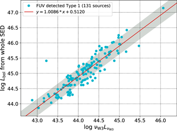
Figure 3. Comparison of monochromatic luminosity in the W3 band,  , and bolometric luminosity estimated from the whole SED, Lbol, for 131 Type 1 AGNs, for which exact measurements (not upper limits) in the FUV band were given in Gupta et al. (2020). The red line corresponds to the linear dependence found between these two parameters via linear regression, and the shaded area illustrates a 1σ confidence interval. Based on such a relation, the bolometric luminosity for all objects in our sample was calculated using Equation (2).
Download figure:
Standard image High-resolution image4.2. BH Mass and Eddington Ratio
In order to obtain BH masses in a uniform way for all AGNs in our sample, we decided to use the relation between BH masses and NIR luminosities of the host galaxies (Marconi & Hunt 2003), with the NIR data being taken from the Two Micron All Sky Survey (Skrutskie et al. 2006). The formula used for our calculations is given as  (Graham 2007), where MK is the absolute K-band magnitude of the galaxy. A more specific explanation of this strategy is given in Gupta et al. (2020, see Appendix A therein).
Having calculated bolometric luminosities and BH masses, we obtained the Eddington ratio as  , where LEdd is the Eddington luminosity. Its values for the whole sample range from 0.0004 ≤ λEdd ≤ 0.1905,10
with a median value of λEdd = 0.011, and its distribution is presented in the top histogram of Figure 4.
, where LEdd is the Eddington luminosity. Its values for the whole sample range from 0.0004 ≤ λEdd ≤ 0.1905,10
with a median value of λEdd = 0.011, and its distribution is presented in the top histogram of Figure 4.

Figure 4. Dependence of the Pj/Lbol ratio on the Eddington ratio λEdd. The sample of 257 radio-detected AGNs has been divided on the basis of how accurate the calculation of jet powers is, i.e., whether the radio emission from lobes can be extracted. The two main groups correspond to lobed sources, which are represented as filled colorful circles (40 objects altogether); and nonlobed radio sources, which are shown as filled colorful triangles (217 objects). Different colors for the group of lobed sources coincide with the Fanaroff–Riley classification: green for FR II, dark gray for FR I/II, and pink for FR I. Nonlobed radio objects are divided into knotty & compact resolved and unresolved ones with yellow and gray colors, respectively.
Download figure:
Standard image High-resolution image4.3. Jet Power
Among various methods of estimating jet powers of AGNs, we decided to use the one based on the calorimetry of radio lobes, originally formulated by Willott et al. (1999) and modified by Shabala & Godfrey (2013), who, by accounting for radiative losses, delivered a more correct relation. Therefore, the formula adopted by us is given as
where L1.4 is the monochromatic lobe radio luminosity at ν = 1.4 GHz, α = 0.8, and D is the source size.
The conversion from radio luminosity to jet power derived by Shabala & Godfrey (2013) is defined for FR II AGNs. These objects constitute 11% of our sample and limiting to those most powerful radio galaxies would give us information about only a fraction of jetted AGNs, clearly biasing our understanding of the jet production mechanisms in various classes of AGNs. The only way to avoid this confusion is to obtain jet powers for all radio-detected sources in our sample by establishing their upper limits. Hence, three groups can be identified: (i) FR II–type AGNs, (ii) objects with lobed but not FR II–type radio morphologies, and (iii) sources with radio detections but without visible double lobes.
A substantial difference appears in our calculations of lobed and nonlobed sources, as for the latter ones we use their total instead of lobe radio luminosity which was originally introduced in Equation (3) and such a quantity can be estimated only for lobed AGNs. Regarding the extraction of lobe radio luminosities, we ensured (when possible) that it does not include any excess radio emission, such as the set of wings in X-shaped sources farther from the core, the outer pair of lobes in DDRGs, or any other radio emission regions which, based on their location on radio maps, do not belong to the radio lobes. In general, the accuracy of the jet power estimation decreases in each of the groups mentioned in the previous paragraph as we have less information about the exact radio characteristics (morphology, size, and flux) of a given source. All jet power calculations for objects in our sample, scaled by bolometric luminosities, are shown in Figure 4.
Even though the results presented in Figure 4 rely mostly on upper limit estimations of Pj (in 223 out of 257 objects), the bimodal distribution of Pj/Lbol is evident, noticeably separating objects powered by relativistic jets from sources in which the radio emission may be dominated by star formation, shocks generated by winds from accretion disks and their coronas, or by low-power jets (Panessa et al. 2019 and references therein). No strong dependence between the Eddington ratio and scaled jet power is found in our sample.
5. Host Galaxies
Having well-defined radio properties for most of the objects in our sample, we checked what the characteristics of their optical counterparts were, specifically their host galaxy morphologies. In order to accomplish that, we decided to use data from the Hubble Space Telescope (HST), Sloan Digital Sky Survey (SDSS), Panoramic Survey Telescope and Rapid Response System (Pan-STARRS), and ESO archives, finding that such information is available for 248 out of 314 AGNs, for which we were able to determine the host galaxy type spanning the entire range of redshifts of our full sample.11 A detailed description of the data and the procedure used to establish the morphologies of host galaxies is given in Appendix C, and below we describe the most important results.
Based on the appearance of the host galaxy in the optical image, we distinguish five morphological groups: elliptical, lenticular, spiral, distorted, and merger.12 The last two groups refer to galaxies in which we were not able to attribute any of the Hubble morphological types. We call a galaxy distorted when its morphology is disarranged, most probably resulting from galaxy interactions, but with only one nucleus. Galaxies in which two nuclei are present are classified as mergers. Some signs of galactic interactions (like tails, bridges, or small distortions) are also seen in both ellipticals and spirals, constituting ∼11% of each of these types.
In Table 2, we show the above-described host galaxy morphological classification with regard to AGNs with and without powerful jets, represented by RL and RI and RQ sources, respectively. Keeping in mind that we have information for 57% and 83% sources in the RL and in the RI and RQ groups, respectively, we see that the majority of RL objects are found to reside in ellipticals while none are found in spirals, which is not the case for radio-quieter AGNs, where both ellipticals and spirals are present, with a prevalence of the latter. Such an observed lack of spiral morphologies in AGNs with extended radio structures is well documented (e.g., Wilson & Colbert 1995; McLure & Jarvis 2004; Best et al. 2005; Madrid et al. 2006; Wolf & Sheinis 2008) albeit some studies reveal several radio-lobed AGNs showing clear disk and/or spiral morphologies in optical images (see Table 4 in Tadhunter 2016 and references therein). The fraction of objects with disturbed morphologies (distorted and merger) in RL and in RI and RQ AGNs is not very different, being 28% and 21%, respectively.
Table 2. Host Galaxy Morphology of Swift/BAT AGNs of Different Radio Classes
| Radio Class | Host Galaxy Morphology | Total | |||||
|---|---|---|---|---|---|---|---|
| Elliptical | Lenticular | Spiral | Distorted | Merger | Unknown | ||
| RL | 17 | 1 | 7 | 19 | 44 | ||
| RI and RQ | 45 | 5 | 126 |

|
7 | 47 | 270 |
| Total | 62 | 6 | 126 | 47 | 7 | 66 | 314 |
Note. The source attributed to the irregular group is indicated by a star. The detailed description of host galaxies is given in Section 5.
Download table as: ASCIITypeset image
We note that our results on host galaxies of Swift/BAT AGNs and their relation to radio properties should be treated as the first step toward more extensive research, which we plan to proceed with in the future.
6. Theoretical Implications
While a consensus is almost reached that relativistic jets in RL AGNs are produced involving the Blandford–Znajek (BZ) mechanism (see review by Blandford et al. 2019 and references therein), we are still lacking answers for such basic questions as
- (1)what is the dominant driver of the very large diversity of jet production efficiencies indicated by radio observations?
- (2)is there any threshold required for the production of jets in RL AGNs?
- (3)are the weak jets observed in some RQ AGNs produced by the same mechanism as RL AGNs?
- (4)why are powerful jets preferentially produced in AGNs hosted by elliptical galaxies?
Noting that the rate of energy extraction from rotating BHs by the BZ mechanism is  , where 0 < a < 1 is the dimensionless BH spin and ΦBH is the magnetic flux confined on the BH by the accretion flow, one may investigate the two following "edge" scenarios to try to explain the diversity of jet production efficiency: the "spin paradigm"—according to which the diversity of the energy extraction rate is driven by the spread in BH spins—and the "magnetic flux paradigm"—where the diversity is determined by the amount of magnetic flux threading the BH.
6.1. Spin Paradigm?
Albeit very popular (Wilson & Colbert 1995; Sikora et al. 2007; Fanidakis et al. 2011; Schulze et al. 2017, and references therein), the "spin paradigm" is seriously challenged by the fact that in order to explain the spread of the jet production efficiency by at least three orders of magnitude, the average BH spin in RQ AGNs should be smaller than 0.03, while that estimated using the "Soltan-type argument" is predicted to be ∼0.6 (Soltan 1982; Chokshi & Turner 1992; Small & Blandford 1992; Elvis et al. 2002; Yu & Tremaine 2002; Lacy et al. 2015). Similarly, large BH spins were found by simulations of the cosmological evolution of BHs (Volonteri et al. 2007, 2013). Hence, in order to reconcile the spin paradigm with RQ AGNs having spins as large as ∼0.6, the dependence of the jet production efficiency on the spin for larger values should be much stronger than quadratic. That possibility was recently claimed to be achievable by Ünal & Loeb (2020) in the model, according to which magnetic fields threading the BH are anchored in the accretion disk. However, noting that magnetic tubes generated in the accretion disk carry on average zero magnetic flux, the jet is predicted to be produced in a flaring fashion (see, e.g., Yuan et al. 2019; Mahlmann et al. 2020) and the resulting time-averaged jet powers can be much smaller than deduced from observations.
6.2. Magnetic Flux Paradigm?
The above might imply that the large diversity of the jet production efficiency is primarily determined by the amount of magnetic flux collected on the BH. However, in order to convert the electromagnetic outflow generated by the BZ mechanism into narrow, relativistic jets, external confinement is required (Beskin et al. 1998; Chiueh et al. 1998; Lyubarsky & Eichler 2001). Such confinement can be provided by magnetohydrodynamic (MHD) outflows from accretion disks and in the case of powerful jets is presumably associated with magnetically arrested disks (MADs; e.g., Narayan et al. 2003; Tchekhovskoy et al. 2011; McKinney et al. 2012). Because MADs are formed only if the centrally accumulated magnetic flux exceeds the maximum amount that can be confined on the BH by the accretion flow, the division of AGNs into RL and RI/RQ ones is likely to correspond to the division of AGNs with and without MADs, or, equivalently, that the formation of the MAD provides a sort of threshold for launching powerful relativistic jets.
6.3. Jet Powers in AGNs with MADs
In order to reconcile such an "MAD/non-MAD" bimodality with our calculated distribution of the jet production efficiency tracer Pj/Lbol (see Figure 4), we need to explain what is the cause of the 2 dex span of this ratio for the RL AGNs assuming they all have MADs. Such a large spread can be an artifact resulting from the calculation of jet powers using their statistical correlation with their radio luminosities (Willott et al. 1999). While adequate in a statistical sense, the conversion formula based on such a correlation may give very large errors for individual sources. Those errors can be associated with the possible spread of parameters such as matter content, minimum electron energy (Willott et al. 1999), cooling effects (Shabala & Godfrey 2013), and density of the environment into which the lobes are inflated (Hardcastle & Krause 2013). But an intrinsic spread of the jet powers in MAD AGNs is also expected, contributed to by the spreads in the BH spin and in the efficiency of the jet collimation by the MHD outflows powered by MADs of different sizes.
It is encouraging to see a similar distribution of Pj/Lbol for our RL AGN sample (Figure 4) and for those found by van Velzen & Falcke (2013) and Inoue et al. (2017) for RLQs. They all peak at Pj/Lbol ∼ 0.1 despite the AGNs included in these samples covering very different accretion rates (see also Rusinek et al. 2017, where four various samples of RL AGNs were studied). Such an average value of the jet production efficiency is smaller by a factor ∼100 than the maximum predicted for MAD AGNs by numerical simulations (e.g., Tchekhovskoy et al. 2011). However it should be noted that the fraction of maximal magnetic flux confined on the BH by the accretion flow depends on the geometrical thickness of the accretion flow (see Avara et al. 2016) and that  (i.e.,
  for
for  ) is achievable only for geometrically thick accretion flows, which are not representative for our AGNs nor for quasars.
6.4. Jets in RQ AGNs
As we can see in Table 1, whereas most of the RL AGNs in our sample are extended (40/44), most RI AGNs are compact (15/20). Hence, there is no doubt that the deficiency of RI AGNs with extended structures is real. Such a deficiency does not mean that there is some threshold for operation of the BZ mechanism, but may simply reflect the very inefficient collimation in AGNs without the help of MHD winds from MADs. Then, the badly collimated BZ outflows would be significantly entrained by winds from stars enclosed within the outflow volume, slowed down and shocked, and then most of their kinetic energy would be expected to be converted to plasma heat, rather than used to accelerate relativistic electrons producing synchrotron radiation. Such radio sources, together with accretion disk coronas, presumably represent the compact radio sources observed in RQ and RI AGNs, with others being associated with star formation rates and accretion disk winds/jets (see review by Panessa et al. 2019 and references therein). Some insights into the nature of compact radio sources of RQ Swift/BAT AGNs are provided by Smith et al. (2016, 2020).
6.5. Building Up the MAD
One can envision the following scenarios to form a MAD: by advection of the magnetic flux by accretion flows, by the accumulation of sufficiently large magnetic flux in a galactic core prior to triggering the AGN phase, and by building up the MAD by the so-called "Cosmic Battery" (CB).
Advection of poloidal magnetic fields by accretion disks was predicted to be very efficient by Bisnovatyi-Kogan & Ruzmaikin (1976). Such a possibility was questioned by Lubow et al. (1994), who pointed out that due to the diffusion of magnetic fields in turbulent plasma, such advection cannot proceed in geometrically thin disks. As later studies showed, poloidal magnetic fields can be advected by the surface layers of accretion disks (Bisnovatyi-Kogan & Lovelace 2007; Rothstein & Lovelace 2008; Guilet & Ogilvie 2012, 2013; Zhu & Stone 2018; Cao & Lai 2019). However, the efficiency of such advection can be limited at distances at which models of thin accretion disks predict their fragmentation due to gravitational instabilities (e.g., Hure et al. 1994; Goodman 2003) and ambipolar diffusion in the outer, only partially ionized portions of the accretion flow (e.g., Begelman 1995). Finally, the advected poloidal magnetic field can be multipolar, and therefore, the formation of a unipolar magnetosphere over the BH and in the innermost portions of the accretion disk—the basic attributes of the MAD—may require more time than the typical lifetime of the AGN, tAGN. Then, only AGNs that are at the age tAGN > ΔtMAD can produce powerful jets, where ΔtMAD is the time it takes to form the MAD. This possibility seems to be supported by noting that the typical lifetimes of FR II sources are ∼3 × 10⁷ yr (e.g., Bird et al. 2008), while the lifetimes of RQ AGNs are presumably much shorter (e.g., Schawinski et al. 2015; Schmidt et al. 2018; Khrykin et al. 2019). However, it should be noted that the prevalence of MADs in ellipticals over disk galaxies, despite their AGNs having similar lifetimes, can be explained by a larger amount of advected magnetic flux per unit mass in the former.
Regarding the second scenario, Sikora et al. (2013) proposed that the central accumulation of magnetic flux occurs during a hot accretion phase, prior to a cold, higher accretion rate "event" representing the AGN phase. As suggested by Sikora & Begelman (2013), such an event might be triggered by the merger of a giant elliptical galaxy with a disk galaxy.
Finally, MADs can be formed locally via the operation of the CB (Contopoulos & Kazanas 1998; Koutsantoniou & Contopoulos 2014; Contopoulos et al. 2018). The model is based on the Poynting–Robertson radiation drag effect, which generates a nonzero component of the toroidal electric field in the innermost regions of the accretion flow, which in turn gives rise to the growth of poloidal magnetic field loops. Assuming that the outer parts of the loops diffuse outwards, the inner parts must then accumulate onto the BH. The possibility of the formation of a MAD by the CB was numerically confirmed by general-relativistic magnetohydrodynamic (GRMHD) simulations (Contopoulos et al. 2018), though so far only for nonrotating BHs and optically thin accretion flows. Unfortunately, the analytically estimated timescales for building up the MAD for BHs with masses larger than 109 M⊙ exceeds the Hubble time (Contopoulos et al. 2018). But, noting that the Poynting–Robertson effect can be much stronger in the case of counterrotating disks, one cannot exclude the formations of MADs in such AGNs within their lifetime. Combining this possibility with predictions that counterrotating configurations can only be formed following mergers involving giant ellipticals with gas-rich spirals (Garofalo et al. 2020), one can explain why RL AGNs are extremely rarely hosted by spiral galaxies (see Section 5). Furthermore, because the fraction of counterrotating disks formed in such mergers is expected to be <50%, one can also explain why RQ AGNs can be found in both ellipticals and spirals.13
7. Summary
In this paper, we investigate in detail the radio properties of massive AGNs ( ) studied by Gupta et al. (2020) and selected from the Swift/BAT catalog (Ricci et al. 2017). Such a sample is excellent for justifying the radio bimodality, claimed by some but questioned by others, and the resulting diversity of jet production efficiency for several reasons. First of all, by selecting via matching the Swift/BAT sources with galaxies, one is avoiding biases associated with radio and optical selection effects; second, most objects in our sample are located at redshifts z < 0.2, which allows for the study of their radio and optical morphologies; third, by excluding high accretion rates, we allow the calculation of masses of their host galaxies and, consequently, BH masses using NIR luminosities; fourth, having the radiative output of our objects be dominated by the MIR, given by WISE, and hard X-rays, given by BAT, allowed for reliable estimations of bolometric luminosities; and finally, by excluding Compton-thick AGNs in our sample, we were able to verify the isotropy of some radiative features by comparing them to Type 1 and Type 2 AGNs (see Gupta et al. 2020). Obviously, due to the very low sensitivity of Swift/BAT, the size of our sample is very much limited, and therefore, the presented results must be treated with some caution, but at the same time, they show incredible potential for future use of AGNs selected by the eROSITA survey.
Our main results and their interpretation can be summarized as follows:
- 1.the distribution of radio loudness in our studied Swift/BAT AGN sample studied is bimodal, with the RL AGNs being on average 500 times radio-louder than RQ AGNs;
- 2.assuming the same relation between radio luminosity and jet power for the entire sample, the distribution of jet production efficiency and of its upper limits were determined;
- 3.a deficiency of jets with intermediate jet production efficiency implies the existence of threshold conditions for the production of powerful jets;
- 4.our premise is that such conditions can be associated with the formation of MADs and that only those AGNs that live longer than the time required to build up the MAD can become RL;
- 5.the extremely rare cases of having RL AGNs hosted by spiral galaxies and having RQ AGNs hosted by both spiral and elliptical galaxies seem to favor the scenario where the MAD is built up by the CB and can be accomplished within the AGN lifetime only in AGNs with accretion disks rotating in the opposite direction to the BH.
We thank David Abarca for useful discussions and editorial assistance. The research leading to these results has received funding from the Polish National Science Centre grant 2016/21/B/ST9/01620 and NAWA (Polish National Agency for Academic Exchange) grant PPN/IWA/2018/1/00100.
Facilities: Based on observations made with the NASA/ESA Hubble Space Telescope - , and obtained from the Hubble Legacy Archive - , which is a collaboration between the Space Telescope Science Institute (STScI/NASA) - , the Space Telescope European Coordinating Facility (ST-ECF/ESA), and the Canadian Astronomy Data Centre (CADC/NRC/CSA). -
Funding for the Sloan Digital Sky Survey IV has been provided by the Alfred P. Sloan Foundation, the US Department of Energy Office of Science, and the Participating Institutions. SDSS-IV acknowledges support and resources from the Center for High-Performance Computing at the University of Utah. The SDSS website is www.sdss.org.
SDSS-IV is managed by the Astrophysical Research Consortium for the Participating Institutions of the SDSS Collaboration including the Brazilian Participation Group, the Carnegie Institution for Science, Carnegie Mellon University, the Chilean Participation Group, the French Participation Group, Harvard-Smithsonian Center for Astrophysics, Instituto de Astrofísica de Canarias, The Johns Hopkins University, Kavli Institute for the Physics and Mathematics of the Universe (IPMU)/University of Tokyo, the Korean Participation Group, Lawrence Berkeley National Laboratory, Leibniz Institut für Astrophysik Potsdam (AIP), Max-Planck-Institut für Astronomie (MPIA Heidelberg), Max-Planck-Institut für Astrophysik (MPA Garching), Max-Planck-Institut für Extraterrestrische Physik (MPE), National Astronomical Observatories of China, New Mexico State University, New York University, University of Notre Dame, Observatário Nacional/MCTI, The Ohio State University, Pennsylvania State University, Shanghai Astronomical Observatory, United Kingdom Participation Group, Universidad Nacional Autónoma de México, University of Arizona, University of Colorado Boulder, University of Oxford, University of Portsmouth, University of Utah, University of Virginia, University of Washington, University of Wisconsin, Vanderbilt University, and Yale University.
The Pan-STARRS1 Surveys (PS1) and the PS1 public science archive have been made possible through contributions by the Institute for Astronomy, the University of Hawaii, the Pan-STARRS Project Office, the Max-Planck Society and its participating institutes, the Max Planck Institute for Astronomy, Heidelberg and the Max Planck Institute for Extraterrestrial Physics, Garching, The Johns Hopkins University, Durham University, the University of Edinburgh, the Queen's University Belfast, the Harvard-Smithsonian Center for Astrophysics, the Las Cumbres Observatory Global Telescope Network Incorporated, the National Central University of Taiwan, the Space Telescope Science Institute, the National Aeronautics and Space Administration under grant No. NNX08AR22G issued through the Planetary Science Division of the NASA Science Mission Directorate, the National Science Foundation grant No. AST-1238877, the University of Maryland, Eotvos Lorand University (ELTE), the Los Alamos National Laboratory, and the Gordon and Betty Moore Foundation.
Appendix A: The Data
A.1. Radio Data
Given that the sources in Gupta et al. (2018) are from the Northern as well as Southern Hemisphere, radio data were collected from two catalogs: NVSS (Condon et al. 1998) and SUMSS (Bock et al. 1999; Mauch et al. 2003). Both are characterized by similar sensitivity (∼2.5 mJy) and resolution (45'' FWHM for NVSS and 45× 45 cosec  arcsec2 for SUMSS). NVSS, a 1.4 GHz continuum survey, covers the northern sky from −40° decl. while SUMSS, a wide-field radio imaging survey conducted at 843 MHz, covers the southern sky from −30° decl., so together they map the whole sky. In addition, we decided to include one more catalog, FIRST (Becker et al. 1995). This 1.4 GHz sky survey is distinguished by its high resolution (5
 4) and its sensitivity down to 1 mJy radio flux. It covers a piece of the sky surveyed by NVSS, and therefore having detections in both of these catalogs helps to determine whether the source is compact or extended, but also to examine the accurate sizes of compact sources (see Appendix B for more details).
For NVSS and SUMSS data, a search within a matching radius of 3' was conducted. For those sources where a single association was found, its exact location was checked—whether the radio match is located within 30'' from the optical center, and if so, this match was assigned to the object. The same procedure was adopted for FIRST data with the only difference being the internal matching radius of 5'' instead of 30''. All the sources having more than one radio association within a matching radius of 3' were checked by eye. This part was done through visual inspection of radio maps with a size of 0 45 × 045 extracted from NVSS,14
SUMSS,15
and FIRST16
by using the NRAO Astronomical Image Processing System17
package. In order to avoid false associations of radio matches, we downloaded the images from DSS1 and DSS2, which are digitized versions of several photographic astronomical surveys, in addition to radio maps, which can be found at the ESO archive.18
Comparison of radio and optical sources on maps from both domains, together with the NASA/IPAC Extragalactic Database,19
enabled us to distinguish incorrect matches. As some sources turned out to have extremely extended, i.e., beyond 3', radio structures we were gradually increasing the radio search by 1' as long as the association for the whole structure was found. Once the whole radio-emitting region was identified, the radio flux of each of the components was summed up and assigned to the given source. For sources lacking radio detections, we assigned them upper limits corresponding to the value of the sensitivity of the survey that contains the source in its footprint. While the sensitivity of NVSS and SUMSS is the same, for objects located in the area covered by both NVSS and FIRST, we decided on FIRST upper limits, as its sensitivity is lower than that of NVSS.
45 × 045 extracted from NVSS,14
SUMSS,15
and FIRST16
by using the NRAO Astronomical Image Processing System17
package. In order to avoid false associations of radio matches, we downloaded the images from DSS1 and DSS2, which are digitized versions of several photographic astronomical surveys, in addition to radio maps, which can be found at the ESO archive.18
Comparison of radio and optical sources on maps from both domains, together with the NASA/IPAC Extragalactic Database,19
enabled us to distinguish incorrect matches. As some sources turned out to have extremely extended, i.e., beyond 3', radio structures we were gradually increasing the radio search by 1' as long as the association for the whole structure was found. Once the whole radio-emitting region was identified, the radio flux of each of the components was summed up and assigned to the given source. For sources lacking radio detections, we assigned them upper limits corresponding to the value of the sensitivity of the survey that contains the source in its footprint. While the sensitivity of NVSS and SUMSS is the same, for objects located in the area covered by both NVSS and FIRST, we decided on FIRST upper limits, as its sensitivity is lower than that of NVSS.
Because the radio catalogs we used were conducted at two different frequencies, the radio fluxes at 843 MHz were recalibrated to 1.4 GHz using a radio spectral index of αr = 0.8 (with the convention of Fν ∝ ν−α) so that the rest of our calculations are consistent.
A.2. Mid-infrared Data
The mid-infrared measurements were taken from the AllWISE Data Release (Cutri et al. 2013) which, by combining data from the cryogenic WISE (Wright et al. 2010) and post-cryogenic NEOWISE ("near-Earth object + WISE," Mainzer et al. 2011) survey phases, resulted in a comprehensive view of the mid-infrared sky. Out of four available bands (at 3.4, 4.6, 12, and 22 μm, corresponding to the W1, W2, W3, and W4 bands, respectively), we decided to make use of the W3 band, which was driven by the fact that at this specific wavelength the dusty torus is transparent enough to observe radiation coming directly from the central region of an AGN. At the shorter wavelengths of the W1 and W2 bands, the dusty, circumnuclear tori are optically thick and radiate anisotropically (Hönig et al. 2011; Netzer 2015). At the longer wavelengths of the W4 band, the dusty torus becomes even more transparent, but its measurements are affected by much larger errors than in W3 because (1) the W4 band traces the warm dust continuum at 22 μm and can be contributed to by starbursts (Ichikawa et al. 2019); (2) the sensitivity in the W4 band is much lower than in the W3 band and its signal-to-noise ratio is the lowest of all the WISE channels, resulting in a lower detected fraction for the objects in our sample; and (3) the resolution of W4 images is worse than in other bands (e.g., 12'' in W4 versus 65 in W3), so for some of our sources (point like in optical, with close neighbors), W4 images could be blended.
Searching for counterparts was conducted within a radius of 5'', which allowed for the avoidance of false matches as the angular resolution of WISE in the W3 band is 65.
The conversion from W3 magnitude, mW3, to the monochromatic flux,  , was done following the formula provided by Wright et al. (2010), given as
  .
.
Appendix B: Size Estimation for Compact AGNs
The radio catalogs we used differ significantly not only in their angular resolutions, and consequently in the accuracy of their fitted deconvolved angular sizes, but also in the data provided for unresolved objects. In NVSS, the angular size is estimated for each object, either as an exact measurement or an upper limit. However, in the case of FIRST and SUMSS, for unresolved sources, a size of 00 is assigned. Therefore, the smallest resolved size listed in each of these catalogs, i.e., 001 and 173 for FIRST and SUMSS, respectively, was taken as an upper limit for unresolved objects detected in these catalogs. Additionally, as was already mentioned in Section 3.1, within a group of 57 compact sources for which data in NVSS and FIRST were available, (1) the angular sizes from NVSS are on average 15 times bigger than those taken from FIRST, and (2) all but five objects are resolved in FIRST (52/57) and only eight are resolved in NVSS (8/57).
Taking into account the above, we decided to use the following procedure to obtain sizes for compact sources:
- 1.for sources having both NVSS and SUMSS measurements, the NVSS size was adopted (eight sources);
- 2.for sources having both NVSS and FIRST measurements, the FIRST size estimate was adopted (57 sources); and
- 3.there are 13 sources with detections only in FIRST, 96 with detections only in NVSS, and 31 with detections only in SUMSS.
Appendix C: Optical Data for Host Galaxy Classification
Optical images for sources in our sample were collected from the following resources: HST through the Hubble Legacy Archive,20 SDSS Data Release 14 (DR14, Abolfathi et al. 2018) through the ImgCutout Web Service,21 and Pan-STARRS (Chambers et al. 2016) through the Image Cutout Server.22 For galaxies that did not have images available in any of those services, we examined (mostly NIR) images retrieved from the ESO Archive Science Portal.23
Similarly to radio data, here we also make use of data differing in angular resolution, optical filter, and sensitivity to extended emission, deciding that the most and the least advantageous information are retrieved from HST and Pan-STARRS data, respectively. This translates to the "importance" of the data in the order of HST as the most reliable, SDSS, and Pan-STARRS as the most uncertain. Objects with data taken from ESO archives are excluded from this "sequence" as (1) they are found in only one resource, and (2) their classification is based on mainly NIR, not optical, images.
Knowing about the origin of the data and based on how many details of the host galaxy can be determined, how accurate the optical images are, and how many of them were available for a given source, we introduced the reliability flag describing the qualitative confidence of our classification. Five groups correspond to the following:
- (1)when the optical images from all three resources were available and the morphology type is obvious and the same in all of them,
- (2)when the optical images from one or two optical resources were available and the morphology type is obvious and the same in all of them,
- (3)when the optical images from two or three resources were available and the morphology type differs between them and is well defined in the image coming from the most credible resource,
- (4)when the optical images from two or three resources were available and the morphology type differs between them and is unreliable in the image coming from the most credible resource,
- (5)when the optical images from one or two resources were available and the morphology type seen there is doubtful.
In general, the reliability of our classification decreases in each of the above groups as it is based on less solid information. Sources with ESO data are assigned to groups 1 or 4 only.
The exact numbers of AGNs flagged as described above are presented in Table C1. A small fraction of all the objects with defined host galaxy morphology belongs to the last three groups corresponding to those with the least reliability (48 out of 248). The classification of most of the sources seem to be quite robust (200 out of 248), although optical images from all three resources exhibiting the same morphological type were only available for a few of them (28 AGNs).
Table C1. The Qualitative Confidence of the Host Galaxy Morphology Classification for 248 AGNs from Our Sample
| Reliability | Host Galaxy Morphology | Total | ||||
|---|---|---|---|---|---|---|
| Elliptical | Lenticular | Spiral | Distorted | Merger | ||
| 0 | 3 | 18 | 6 | 1 | 28 | |
| 1 | 41 | 2 | 94 |

|
6 | 172 |
| 2 | 4 | 4 | 5 | 13 | ||
| 3 | 4 | 2 | 1 | 2 | 9 | |
| 4 | 10 | 2 | 9 | 5 | 26 | |
| Total | 62 | 6 | 126 | 47 | 7 | 248 |
Note. The source attributed to the irregular group is indicated by a star.
Download table as: ASCIITypeset image
Appendix D: The Sample
Table D1 lists the most important information obtained and discussed in this work for some of the sources in our sample of Swift/BAT AGNs. The complete sample is available as supplementary material.
Table D1. Swift/BAT Sample of 314 AGNs Used in This Study
| SWIFT Name | Counterpart Name | z |

|

|

|
Radio |

|
R | Radio | Size |

|
Radio | FRd | Host | Host |
|---|---|---|---|---|---|---|---|---|---|---|---|---|---|---|---|
| Flaga | Classb | Morphologyc | Flage | Morphologyf | |||||||||||
| (M⊙) | (erg s−1) | (mJy) | (kpc) | ||||||||||||
| J1940.4-3015 | IGR J19405–3016 | 0.0525 | 8.72 | 45.08 | −1.75 | N | 9.6 | −0.94 | RQ | 28.96g | <−3.69 | C | P | S | |
| J1952.4+0237 | 3C 403 | 0.0584 | 8.90 | 45.15 | −1.85 | N | 6045.4 | 1.88 | RL | 167.91 | −1.06 | X | II | H | L |
| J1959.4+4044 | Cygnus A | 0.0558 | 9.29 | 45.33 | −2.06 | N | 1598189.0 | 4.09 | RL | 104.65 | 0.60 | D | II | H | E |
| J2001.0-1811 | 2MASX J20005575–1810274 | 0.0372 | 8.57 | 45.27 | −1.40 | U | 2.5 | −2.03 | RQ | H | L | ||||
| J2018.4-5539 | PKS 2014–55 | 0.0607 | 8.86 | 45.05 | −1.91 | S | 1597.5 | 1.44 | RL | 1367.75 | −0.73 | T | I | E | E |
| J2030.2-7532 | IRAS 20247–7542 | 0.114 | 9.02 | 46.09 | −1.03 | S | 8.6 | −1.29 | RQ | 35.80g | <−4.10 | C | |||
| J2033.4+2147 | 4C +21.55 | 0.174 | 9.17 | 45.73 | −1.54 | N | 1940.1 | 1.82 | RL | 544.32 | −1.09 | T | II | P | D |
| J2040.2-5126 | ESO 234–IG 063 | 0.0541 | 8.60 | 45.01 | −1.68 | S | 28.2 | −0.38 | RQ | 18.21g | <−3.35 | C | E | D | |
| J2042.3+7507 | 4C +74.26 | 0.105 | 9.32 | 45.90 | −1.52 | N | 1894.0 | 1.16 | RL | 1140.84 | −1.27 | T | II | ||
| J2044.2-1045 | Mrk 509 | 0.0344 | 8.72 | 45.19 | −1.63 | N | 18.6 | −1.15 | RQ | 15.42 | <−4.05 | C | H | S | |
| J2052.0-5704 | IC 5063 | 0.0115 | 8.56 | 44.74 | −1.92 | S | 1448.5 | 0.23 | RI | 9.53 | <−2.99 | K | H | E | |
| J2109.2+3531 | B2 2107+35A | 0.202 | 9.30 | 45.88 | −1.52 | N | 1434.4 | 1.69 | RL | 344.87 | <−1.06 | K | |||
| J2114.4+8206 | 2MASX J21140128+8204483 | 0.0833 | 8.87 | 45.41 | −1.57 | N | 474.9 | 0.84 | RI | 308.21 | −2.05 | T | I | P | E |
| J2116.3+2512 | 2MASX J21161028+2517010 | 0.153 | 8.62 | 45.05 | −1.67 | U | 2.5 | −0.51 | RQ | ||||||
| J2118.9+3336 | 2MASX J21192912+3332566 | 0.0509 | 8.69 | 44.33 | −2.46 | N | 3.7 | −0.63 | RQ | 138.17g | <−2.91 | C | P | E | |
| J2134.9-2729 | 2MASX J21344509–2725557 | 0.0667 | 8.74 | 45.00 | −1.84 | N | 7.8 | −0.74 | RQ | 118.52 | <−3.16 | C | P |

|
|
| J2135.5-6222 | 1RXS J213623.1–622400 | 0.059 | 8.72 | 45.17 | −1.65 | S | 4.3 | −1.28 | RQ | 19.74g | <−4.08 | C | |||
| J2137.8-1433 | PKS 2135–14 | 0.2 | 9.19 | 45.95 | −1.34 | N | 3864.0 | 2.04 | RL | 365.62 | −0.78 | D | II | ||
| J2145.5+1101 | RX J2145.5+1102 | 0.209 | 8.73 | 45.25 | −1.57 | F | 1.1 | −0.77 | RQ | 16.66 | <−3.67 | C | |||
| J2150.2-1855 | 6dF J2149581–185924 | 0.158 | 8.68 | 45.26 | −1.53 | N | 528.4 | 1.64 | RL | 220.81 | <−1.11 | C | |||
| J2157.2-6942 | PKS 2153-69 | 0.0283 | 8.81 | 44.21 | −2.71 | S | 29203.8 | 2.86 | RL | 37.42 | −0.33 | T | II | H | E |
| J2200.9+1032 | Mrk 520 | 0.0275 | 8.54 | 44.78 | −1.86 | F | 60.8 | −0.42 | RQ | 1.57 | <−3.97 | C | S | D | |
| J2204.7+0337 | 2MASX J22041914+0333511 | 0.0611 | 8.89 | 45.58 | −1.41 | F | 8.8 | −1.35 | RQ | 0.01g | <−6.08 | C | S | D | |
| J2209.1-2747 | NGC 7214 | 0.0227 | 8.87 | 44.38 | −2.59 | N | 28.2 | −0.52 | RQ | 13.66 | <−3.42 | C | P | S | |
| J2214.2-2557 | 2MASX J22140917–2557487 | 0.0519 | 8.70 | 44.36 | −2.45 | N | 3.1 | −0.72 | RQ | 60.34g | <−3.19 | C | P | S | |
| J2217.0+1413 | Mrk 304 | 0.0704 | 8.96 | 45.26 | −1.80 | U | 2.5 | −1.44 | RQ | ||||||
| J2223.9-0207 | 3C 445 | 0.0601 | 8.54 | 45.43 | −1.21 | N | 5783.9 | 1.60 | RL | 660.07 | −1.15 | X | II | ||
| J2226.8+3628 | MCG +06-49-019 | 0.0213 | 8.61 | 43.64 | −3.07 | N | 7.0 | −0.44 | RQ | 18.96g | <−3.13 | C | S | S | |
| J2234.8-2542 | ESO 533–G 050 | 0.0265 | 8.67 | 43.53 | −3.24 | U | 2.5 | −0.59 | RQ | P | S | ||||
| J2235.9+3358 | NGC 7319 | 0.0227 | 8.63 | 44.28 | −2.44 | N | 53.0 | −0.15 | RQ | 34.71 | <−2.87 | C | H |

|
|
| J2246.0+3941 | 3C 452 | 0.0811 | 8.79 | 44.96 | −1.93 | N | 10556.6 | 2.62 | RL | 316.76 | −0.40 | T | II | H | E |
| J2248.7-5109 | 2MASX J22484165–5109338 | 0.1 | 8.52 | 45.34 | −1.28 | U | 2.5 | −1.20 | RQ |
Notes. This subset of the table demonstrates format and content.
aOrigin of the radio flux: N—NVSS; S—SUMSS; F—FIRST; U—undetected. bRL—radio loud; RI—radio intermediate; RQ—radio quiet. cX—complex; T—triple; D—double; K—knotty; C—compact. dOur Fanaroff–Riley classification for lobed sources only. eOrigin of the host morphology classification: H—HST; S—SDSS; P—Pan-STARRS; E—ESO. fE—elliptical; L—lenticular; S—spiral; D—distorted; Irr—irregular; M—merger. The subscript "i" indicates interacting galaxies. gCompact unresolved sources for which their angular sizes equal the upper limits obtained from a given catalog (Appendix B).Only a portion of this table is shown here to demonstrate its form and content. A machine-readable version of the full table is available.
Download table as: DataTypeset image
Footnotes
- 4
Those are taken from NVSS, FIRST, and SUMSS, where radio fluxes from the latest, at 843 MHz, were recalibrated to 1.4 GHz using a radio spectral index of αr = 0.8 and the convention of
 see Appendix A.1.
 - 5
The exception being the group of 57 compact sources, for which, even though they have data in both, NVSS and FIRST, we decided to take the FIRST fluxes. The explanation is given in Appendix B. This choice, however, does not affect the ascription to their radio classes.
- 6
Those are PKS 0707–35, B2 1204+34, 3C 403, 3C 445, and PKS 2356–61.
- 7
- 8
Those are 2MASX J03181899+6829322, IGR 14488–4008, Mrk 1498, 4C +34.47, 4C +74.26, and PKS 2356–61.
- 9
The only source not clearly following this trend is LEDA 100168 (
, log Lbol = 45.41). - 10
The difference between the ranges of λEdd in our and the Gupta et al. (2020) studies results from different methods of Lbol estimation.
- 11
In fact, all of our objects were found in the given surveys but not all of them had good-enough data to establish their host morphology resulting in the exclusion of 66 objects.
- 12
Additionally, we identify one more group, irregular, consisting of only one source, 2MASX J23444387–4243124. We include this object in the distorted group.
- 13
The idea of having RL AGNs associated with BHs and accretion disks rotating in opposite directions to each other is not new. It was proposed by Garofalo et al. (2010), based on the works by Reynolds et al. (2006) and Garofalo (2009a, 2009b), who argued that jets produced by the BZ mechanism are more powerful in systems with retrograde disks than in systems with prograde disks. They suggested that this can explain the radio bimodality of AGNs. However, GRMHD simulations showed that the largest jet powers are achievable not in retrograde configurations but in prograde configurations (Tchekhovskoy & McKinney 2012; Tchekhovskoy et al. 2012). This might suggest that opposite to what was proposed by Garofalo et al., RL AGNs should be associated with prograde disks, and, therefore, the fraction of AGNs with retrograde disks should be much larger than the fraction of AGNs with prograde disks. However, the difference of maximal jet powers (those produced assuming the MAD models) produced by AGNs with retro- and prograde disks is much too small (only by a factor ∼3) to explain the observed jet production diversity and, therefore, cannot be responsible for the radio-loudness distribution with RL and RQ peaks observed to be separated by a factor of ∼500.
- 14
- 15
- 16
- 17
- 18
- 19
- 20
- 21
- 22
- 23

